
Intelligent Dynamic Identification Technique of Industrial Products in a Robotic Workplace

 ,
,  ,
, 
Abstract
:1. Introduction
2. Subject and Methods
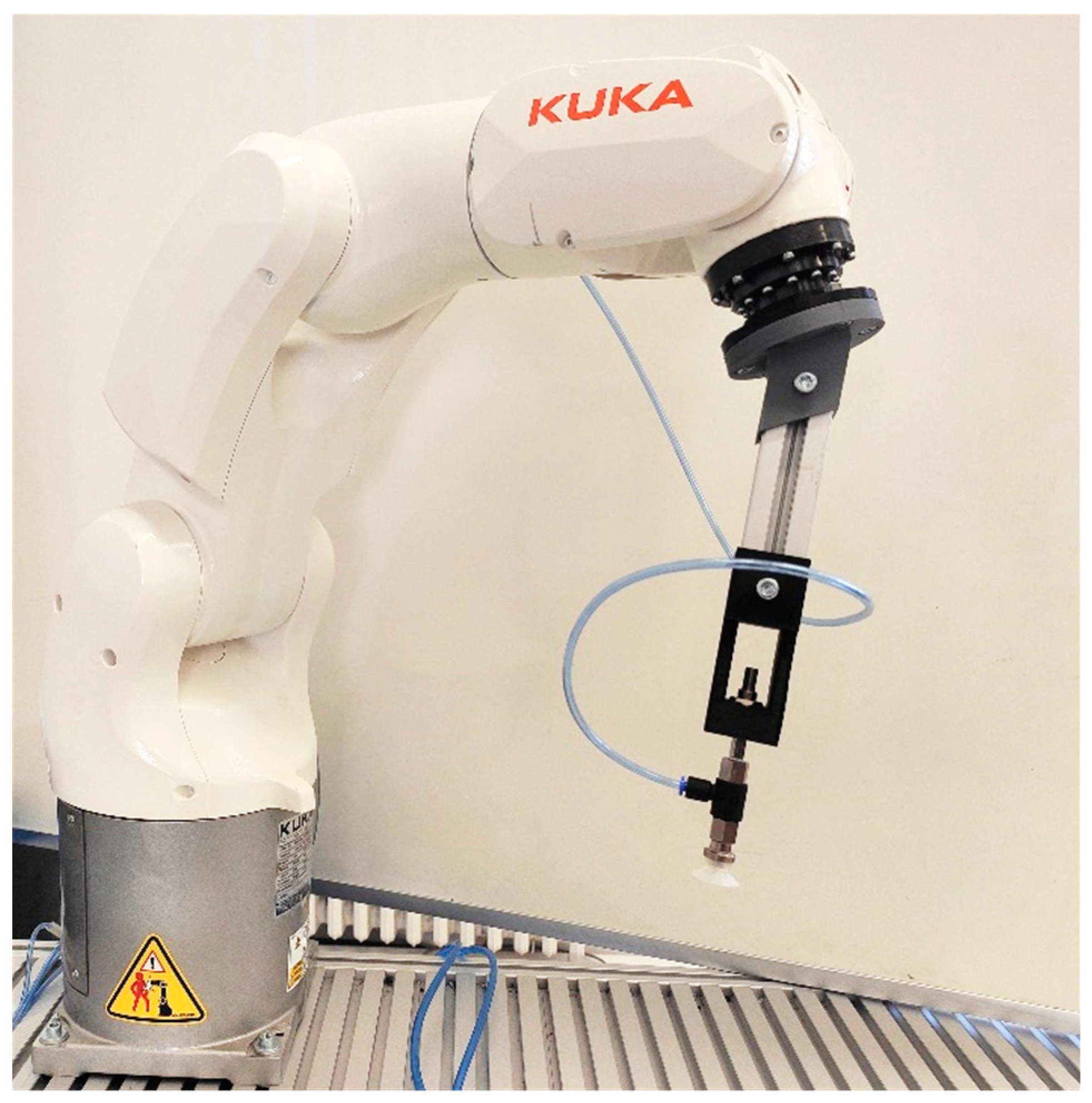
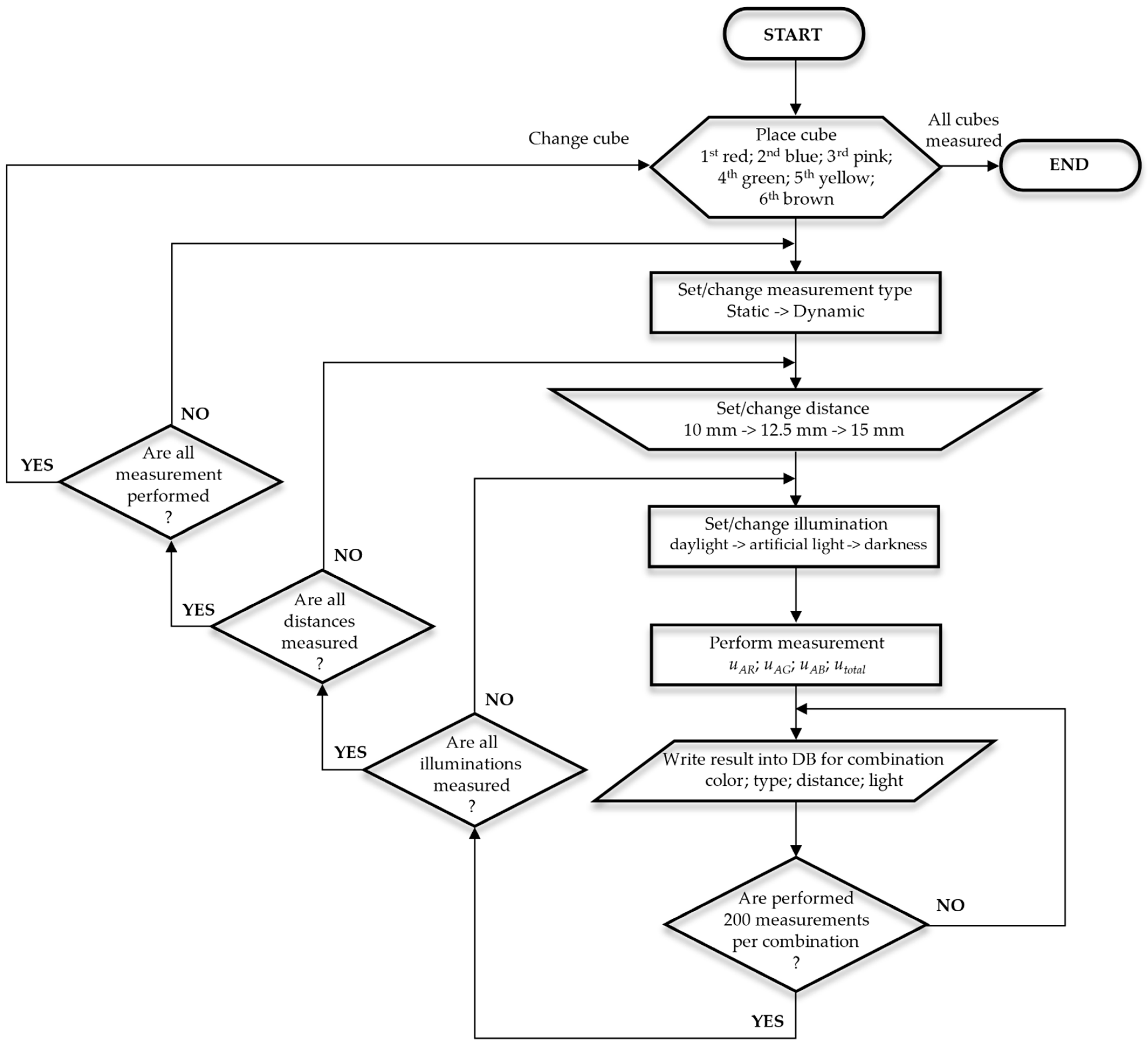
Preparation of Test Robotic Workplace
3. Results
3.1. Statistical Evaluation of Measured Data
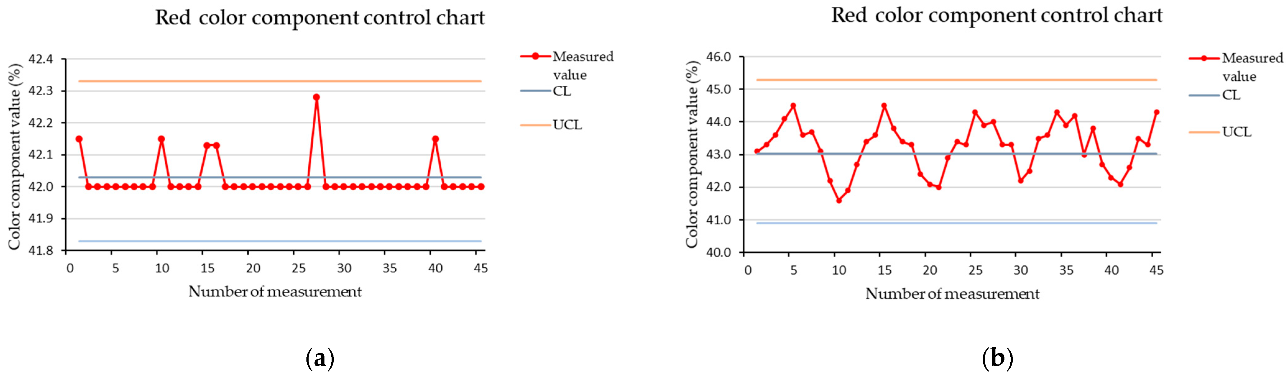
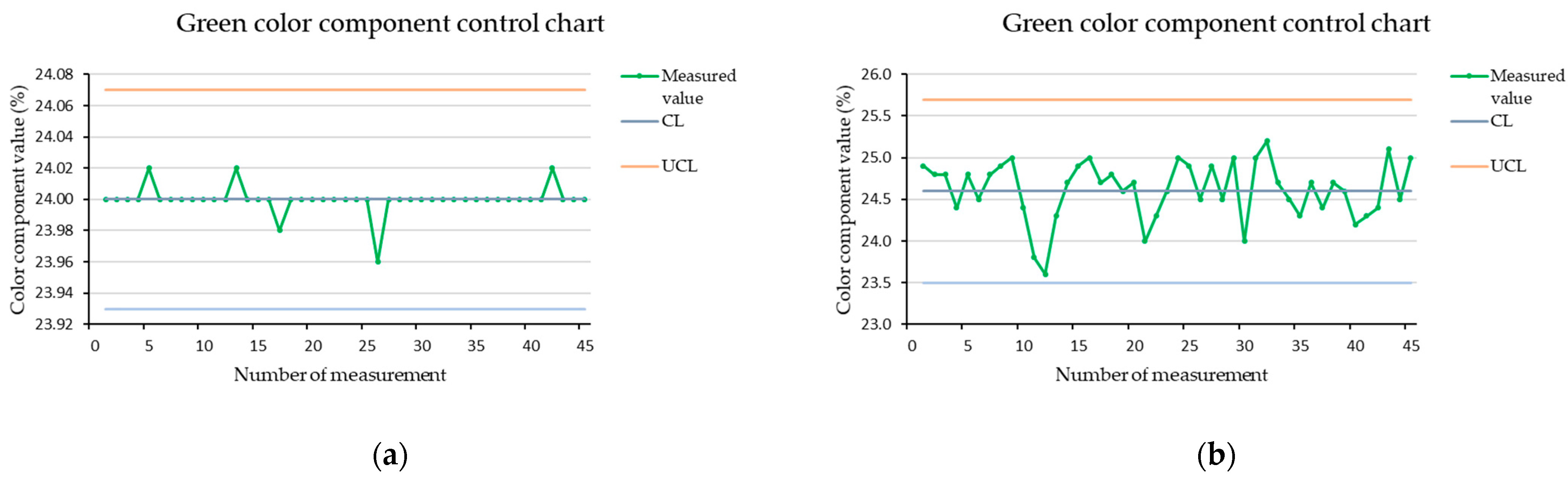
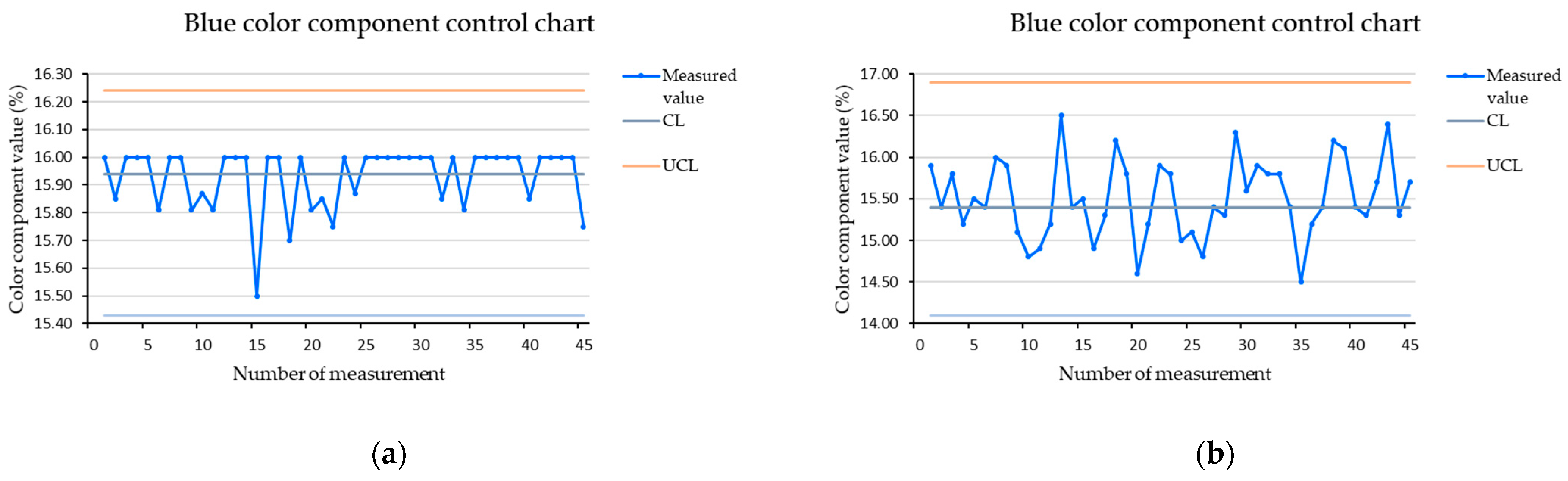
3.2. Definition of Control Limits and Control Chart Creation
3.3. RGB Color Component Charts for Measurement of Stopped Brown Cube
3.4. Stability Monitoring of the Measuring Process
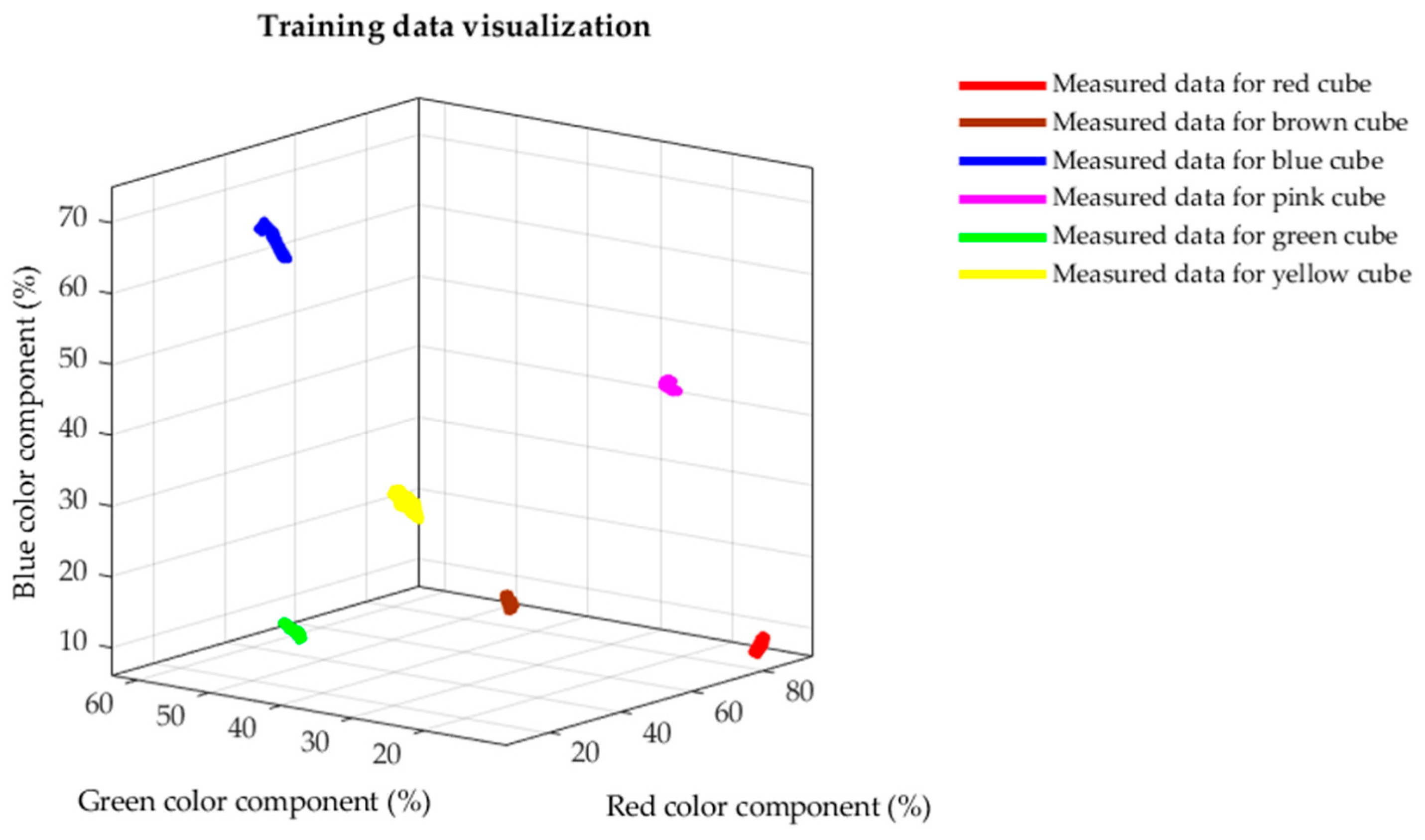
3.5. K-Nearest Neighbors Algorithm for Identification of Values Outside the Control Limits
- Conveyor belt speed;
- Illumination;
- Scanning distance;
- Measured value of red, blue and green color component.
4. Discussion
Author Contributions
Funding
Institutional Review Board Statement
Informed Consent Statement
Data Availability Statement
Conflicts of Interest
References
- Sardar, S.K.; Sarkar, B.; Kim, B. Integrating Machine Learning, Radio Frequency Identification, and Consignment Policy for Reducing Unreliability in Smart Supply Chain Management. Processes 2021, 9, 247. [Google Scholar] [CrossRef]
- Tran, N.-H.; Park, H.-S.; Nguyen, Q.-V.; Hoang, T.-D. Development of a Smart Cyber-Physical Manufacturing System in the Industry 4.0 Context. Appl. Sci. 2019, 9, 3325. [Google Scholar] [CrossRef] [Green Version]
- Gardner, H.; Kleiner, F.S.; Mamiya, C.J.; Tansey, G.T. Gardner’s Art through the Ages, 11th ed.; Harcourt College Publishers: Fort Worth, TX, USA, 2001. [Google Scholar]
- Makbkhot, M.M.; Al-Ahmari, A.M.; Salah, B.; Alkhalefah, H. Requirements of the Smart Factory System: A Survey and Perspective. Machines 2018, 6, 23. [Google Scholar] [CrossRef] [Green Version]
- Kritzinger, W.; Karner, M.; Traar, G.; Henjes, J.; Sihn, W. Digital Twin in manufacturing: A categorical literature review and classification. IFAC PapersOnLine 2018, 51, 1016–1022. [Google Scholar] [CrossRef]
- Tao, F.; Zhang, H.; Liu, A.; Nee, A.Y.C. Digital Twin in Industry: State-of-the-Art. IEEE Trans. Ind. Inform. 2019, 15, 2405–2415. [Google Scholar] [CrossRef]
- Cohen, Y.; Naseraldin, H.; Chaudhuri, A.; Pilati, F. Assembly systems in Industry 4.0 era: A road map to understand Assembly 4.0. Int. J. Adv. Manuf. Technol. 2019, 105, 4037–4054. [Google Scholar] [CrossRef]
- Valencia, E.T.; Lamouri, S.; Pellerin, R.; Dubois, P.; Moeuf, A. Production Planning in the Fourth Industrial Revolution: A Literature Review. IFAC PapersOnLine 2019, 52, 2158–2163. [Google Scholar] [CrossRef]
- Burmester, M.; Munilla, J.; Ortiz, A.; Caballero-Gil, P. An RFID-Based Smart Structure for the Supply Chain: Resilient Scanning Proofs and Ownership Transfer with Positive Secrecy Capacity Channels. Sensors 2017, 17, 1562. [Google Scholar] [CrossRef] [PubMed]
- Benito-Altamirano, I.; Pfeiffer, P.; Cusola, O.; Daniel Prades, J. Machine-Readable Pattern for Colorimetric Sensor Interrogation. Proceedings 2018, 2, 906. [Google Scholar] [CrossRef] [Green Version]
- Kang, H.R. Color Technology for Electronic Imaging Devices; SPIE Optical Engineering Press: Bellingham, WA, USA, 1997. [Google Scholar]
- Ford, A.; Roberts, A. Colour Space Conversions; Westminster University: London, UK, 1998. [Google Scholar]
- International Colour Consortium (ICC). Available online: http://www.color.Org/faqs.xalter#wh2 (accessed on 14 February 2021).
- Menesatti, P.; Angelini, C.; Pallottino, F.; Antonucci, F.; Aguzzi, J.; Costa, C. RGB Color Calibration for Quantitative Image Analysis: The “3D Thin-Plate Spline” Warping Approach. Sensors 2012, 12, 7063–7079. [Google Scholar] [CrossRef] [Green Version]
- Okfalisa; Gazalba, I.; Mustakim, M.; Reza, N.G.I. Comparative analysis of k-nearest neighbor and modified k-nearest neighbor algorithm for data classification. In Proceedings of the 2nd International conferences on Information Technology, Information Systems and Electrical Engineering (ICITISEE), Yogyakarta, Indonesia, 1–3 November 2017; pp. 294–298. [Google Scholar] [CrossRef]
- Ohmori, S.A. Predictive Prescription Using Minimum Volume k-Nearest Neighbor Enclosing Ellipsoid and Robust Optimization. Mathematics 2021, 9, 119. [Google Scholar] [CrossRef]
- Yoo, Y.; Yoo, W.S. Turning Image Sensors into Position and Time Sensitive Quantitative Colorimetric Data Sources with the Aid of Novel Image Processing/Analysis Software. Sensors 2020, 20, 6418. [Google Scholar] [CrossRef]
- KUKA KR3 R540. [online]. © KUKA AG 2020. Available online: https://www.kuka.com/sk-sk/servisn%C3%A9-slu%C5%BEby/downloads?terms=Language:sk:1;Language:en:1Language:en:1&q= (accessed on 29 January 2021).
- Industrial Robots. General Technical Requirements; STN 18 6508; Slovak Office of Standards, Metrology and Testing: Bratislava, Slovakia, 1990; p. 8. [Google Scholar]
- CSM Color Sensor. [online]. © 2020 SICK AG. Available online: https://www.sick.com/ag/en/registration-sensors/color-sensors/csm/c/g305962 (accessed on 29 January 2021).
- Vašek, P. Design of Methodology and Measurement Model for Testing the Logistics System in Flexible Production and Design of Algorithms for its Optimization; SUT: Bratislava, Slovakia, 2020. [Google Scholar]
- Kelemenová, T.; Dovica, M. Gauge Calibration, 1st ed.; Technical University of Košice, Faculty of Mechanical Engineering, Edition of Scientific and Professional Literature: Košice, Slovakia, 2016; p. 232. ISBN 978-80-553-3069-3. [Google Scholar]
- Skibicki, J.; Golijanek-Jędrzejczyk, A.; Dzwonkowski, A. The Influence of Camera and Optical System Parameters on the Uncertainty of Object Location Measurement in Vision Systems. Sensors 2020, 20, 5433. [Google Scholar] [CrossRef] [PubMed]
- Barone, F.; Marrazzo, M.; Oton, C.J. Camera Calibration with Weighted Direct Linear Transformation and Anisotropic Uncertainties of Image Control Points. Sensors 2020, 20, 1175. [Google Scholar] [CrossRef] [PubMed] [Green Version]
- Wimmer, G.; Palenčár, R.; Witkovský, V.; Ďuriš, S. Evaluation of Gauge Calibration: Statistical Methods for Analysis of Uncertainties in Metrology, 1st ed.; SUT: Bratislava, Slovakia, 2015; p. 191. ISBN 978-80-227-4374-7. [Google Scholar]
- Němeček, P. Measurement Uncertainties, 1st ed.; Czech Society for Quality: Praha, Czech Republic, 2008; p. 96. ISBN 978-80-02-02089-9. [Google Scholar]
- Vašek, P.; Rybář, J.; Vachálek, J. Identification of colored objects and factors affecting the control of the measurement process in the experimental workplace. Metrol. Test. 2020, 1, 4–7. [Google Scholar]
- Palenčár, R.; Kureková, E.; Halaj, M. Measurement and Metrology for Managers; SUT: Bratislava, Slovakia, 2007; p. 252. ISBN 978-80-227-2743-3. [Google Scholar]
- Palenčár, R.; Ruiz, J.M.; Janiga, I.; Horníková, A. Statistical Methods in Metrological and Testing Laboratories; SUT: Bratislava, Slovakia, 2001; p. 366. ISBN 80-968449-3-8. [Google Scholar]
- Zheng, N.; Lu, X. Comparative Study on Push and Pull Production System Based on Anylogic. In Proceedings of the International Conference on Electronic Commerce and Business Intelligence, Beijing, China, 6–7 June 2009; pp. 455–458. [Google Scholar] [CrossRef]
- Peng, X.; Chen, R.; Yu, K.; Ye, F.; Xue, W. An Improved Weighted K-Nearest Neighbor Algorithm for Indoor Localization. Electronics 2020, 9, 2117. [Google Scholar] [CrossRef]
- Micieta, B.; Binasova, V.; Lieskovsky, R.; Krajcovic, M.; Dulina, L. Product Segmentation and Sustainability in Customized Assembly with Respect to the Basic Elements of Industry 4.0. Sustainability 2019, 11, 6057. [Google Scholar] [CrossRef] [Green Version]
- Groover, M.P. Automation, Production Systems, and Computer-Integrated Manufacturing; Pearson Education, Inc.: Upper Saddle River, NJ, USA, 2008; ISBN-13>978-0132393218. [Google Scholar]
- Jia, J. A Machine Vision Application for Industrial Assembly Inspection. In Proceedings of the Second International Conference on Machine Vision, Dubai, UAE, 28–30 December 2009; pp. 172–176. [Google Scholar] [CrossRef]
- WU, D.; Sun, D.W. Colour measurements by computer vision for food quality control—A review. Trends Food Sci. Technol. 2013, 29, 5–20. [Google Scholar] [CrossRef]
- Li, J. Application Research of Vision Sensor in Material Sorting Automation Control System. IOP Conf. Ser. Mater. Sci. Eng. 2020, 782, 022074. [Google Scholar] [CrossRef]
- Shrestha, A.; Karki, N.; Yonjan, R.; Subedi, M.; Phuyal, S. Automatic Object Detection and Separation for Industrial Process Automation. In Proceedings of the IEEE International Students’ Conference on Electrical, Electronics and Computer Science (SCEECS), Bhopal, India, 22–23 February 2020; pp. 1–5. [Google Scholar] [CrossRef]
- Mandel, B.J. The Regression Control Chart. J. Qual. Technol. 1969, 1, 1–9. [Google Scholar] [CrossRef]
- Vapnik, V. The Nature of Statistical Learning Theory; Springer Science & Business Media: Berlin, Germany, 2013; ISBN 978-1-4757-3264-1. [Google Scholar]
- Photoneo PhoXi Scaners. Available online: https://www.photoneo.com/phoxi-3d-scanner/ (accessed on 14 February 2021).
- Koori, A.; Anitei, D.; Boitor, A.; Silea, I. Image-Processing-Based Low-Cost Fault Detection Solution for End-of-Line ECUs in Automotive Manufacturing. Sensors 2020, 20, 3520. [Google Scholar] [CrossRef]
- Cognex Vision Pro Deep Learning. Available online: https://www.cognex.com/products/deep-learning/visionpro-deep-learning (accessed on 14 February 2021).


| Maximum reach | 541 mm |
| Payload | 3 kg |
| Pose repeatability | ±0.02 mm |
| Number of axes | 6 |
| Mounting positions | Ceiling, Floor, Wall |
| Footprint | 179 × 179 mm |
| Weigh | 26.5 kg |
| Ambient operatingtemperature | 5 °C–45 °C |
| Protection class | IP40 |
| Controller | KR C-4 compact |
| Length | 1500 mm |
| Width | 25 mm |
| Height | 1000 mm |
| Motor | three-phase motor Nord |
| Control | Siemens Sinamics V20 frequency converter |
| Maximum revolutions | 1415 RPM |
| Belt material | rubber with anti-slip surface |
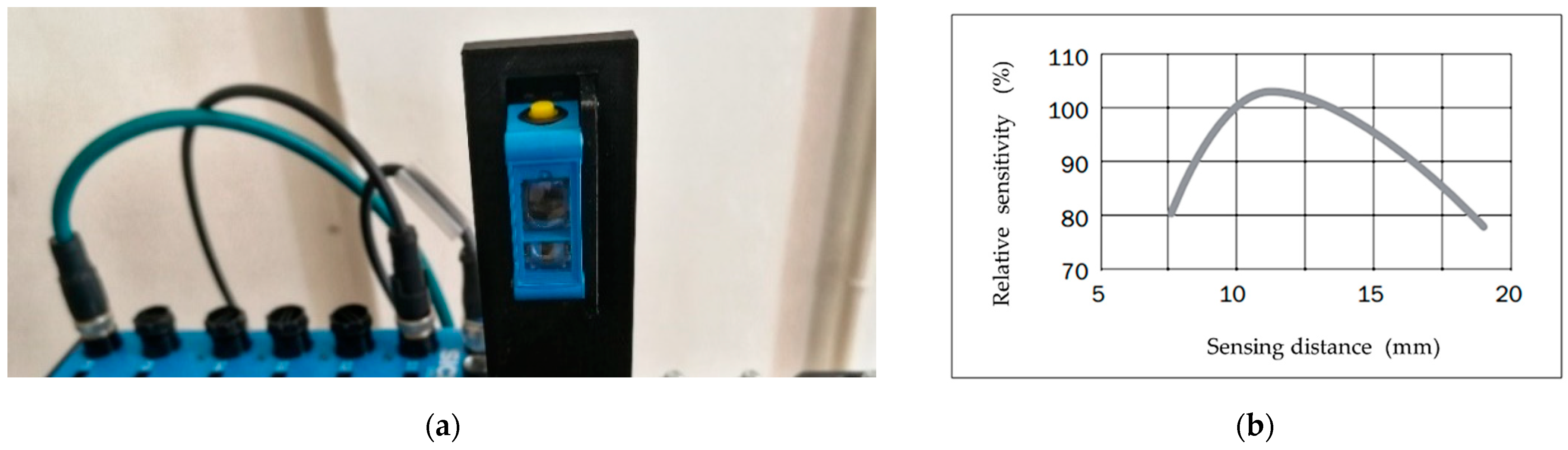
| Dimensions | 22 mm × 12 mm × 32 mm |
| Sensing distance | 12.5 mm |
| Sensing distance tolerance | ±3 mm |
| Light source | Light Emitting Diode (LED), RGB |
| Wave length | 640 nm, 525 nm, 470 nm |
| Light spot size | 1.5 mm × 6.5 mm |
| Response time | 300 µs |
| Supply voltage | DC 12 V ... 24 V |
| Output (channel) | 1 color/8 colors via IO-Link |
| Illumination | Sensor Distance (mm) | Cube Stops | Cube in Motion | ||||||
|---|---|---|---|---|---|---|---|---|---|
| Natural daylight | 10 | 0.010 | 0.005 | 0.011 | 0.016 | 0.105 | 0.021 | 0.026 | 0.110 |
| Natural daylight | 12.5 | 0.001 | 0.007 | 0.011 | 0.013 | 0.079 | 0.031 | 0.034 | 0.091 |
| Natural daylight | 15 | 0.004 | 0.011 | 0.001 | 0.012 | 0.060 | 0.023 | 0.020 | 0.067 |
| Artificial light | 10 | 0.000 | 0.003 | 0.001 | 0.003 | 0.198 | 0.036 | 0.043 | 0.206 |
| Artificial light | 12.5 | 0.002 | 0.003 | 0.001 | 0.004 | 0.458 | 0.041 | 0.051 | 0.463 |
| Artificial light | 15 | 0.004 | 0.001 | 0.011 | 0.012 | 0.065 | 0.030 | 0.028 | 0.077 |
| Darkness | 10 | 0.000 | 0.011 | 0.000 | 0.011 | 0.160 | 0.029 | 0.034 | 0.166 |
| Darkness | 12.5 | 0.016 | 0.000 | 0.008 | 0.018 | 0.064 | 0.025 | 0.027 | 0.074 |
| Darkness | 15 | 0.000 | 0.003 | 0.005 | 0.006 | 0.103 | 0.029 | 0.027 | 0.110 |
| Illumination | Sensor Distance (mm) | Cube Stops | Cube in Motion | ||||||
|---|---|---|---|---|---|---|---|---|---|
| Natural daylight | 10 | 0.000 | 0.004 | 0.022 | 0.022 | 0.021 | 0.093 | 0.259 | 0.276 |
| Natural daylight | 12.5 | 0.011 | 0.003 | 0.004 | 0.012 | 0.020 | 0.027 | 0.049 | 0.059 |
| Natural daylight | 15 | 0.002 | 0.005 | 0.012 | 0.013 | 0.030 | 0.059 | 0.057 | 0.087 |
| Artificial light | 10 | 0.010 | 0.012 | 0.000 | 0.016 | 0.018 | 0.115 | 0.318 | 0.339 |
| Artificial light | 12.5 | 0.002 | 0.006 | 0.008 | 0.010 | 0.018 | 0.018 | 0.056 | 0.062 |
| Artificial light | 15 | 0.014 | 0.000 | 0.007 | 0.016 | 0.052 | 0.106 | 0.106 | 0.159 |
| Darkness | 10 | 0.014 | 0.001 | 0.002 | 0.014 | 0.022 | 0.095 | 0.235 | 0.254 |
| Darkness | 12.5 | 0.001 | 0.007 | 0.004 | 0.008 | 0.024 | 0.030 | 0.027 | 0.047 |
| Darkness | 15 | 0.011 | 0.003 | 0.007 | 0.013 | 0.042 | 0.111 | 0.113 | 0.164 |
| Illumination | Sensor Distance (mm) | Cube Stops | Cube in Motion | ||||||
|---|---|---|---|---|---|---|---|---|---|
| Natural daylight | 10 | 0.003 | 0.005 | 0.000 | 0.006 | 0.119 | 0.035 | 0.066 | 0.141 |
| Natural daylight | 12.5 | 0.005 | 0.008 | 0.019 | 0.021 | 0.197 | 0.043 | 0.137 | 0.244 |
| Natural daylight | 15 | 0.006 | 0.003 | 0.016 | 0.017 | 0.035 | 0.042 | 0.037 | 0.066 |
| Artificial light | 10 | 0.018 | 0.022 | 0.010 | 0.030 | 0.192 | 0.218 | 0.230 | 0.371 |
| Artificial light | 12.5 | 0.000 | 0.015 | 0.019 | 0.024 | 0.213 | 0.084 | 0.131 | 0.264 |
| Artificial light | 15 | 0.006 | 0.007 | 0.012 | 0.015 | 0.077 | 0.053 | 0.036 | 0.100 |
| Darkness | 10 | 0.027 | 0.006 | 0.016 | 0.032 | 0.087 | 0.039 | 0.056 | 0.111 |
| Darkness | 12.5 | 0.000 | 0.014 | 0.014 | 0.020 | 0.149 | 0.028 | 0.074 | 0.169 |
| Darkness | 15 | 0.000 | 0.000 | 0.008 | 0.008 | 0.045 | 0.031 | 0.023 | 0.059 |
| Illumination | Sensor Distance (mm) | Cube Stops | Cube in Motion | ||||||
|---|---|---|---|---|---|---|---|---|---|
| Natural daylight | 10 | 0.007 | 0.012 | 0.001 | 0.014 | 0.028 | 0.093 | 0.048 | 0.108 |
| Natural daylight | 12.5 | 0.011 | 0.002 | 0.017 | 0.020 | 0.021 | 0.031 | 0.020 | 0.042 |
| Natural daylight | 15 | 0.004 | 0.014 | 0.004 | 0.015 | 0.053 | 0.179 | 0.041 | 0.191 |
| Artificial light | 10 | 0.005 | 0.002 | 0.002 | 0.006 | 0.044 | 0.147 | 0.079 | 0.173 |
| Artificial light | 12.5 | 0.014 | 0.019 | 0.012 | 0.026 | 0.023 | 0.034 | 0.027 | 0.049 |
| Artificial light | 15 | 0.001 | 0.016 | 0.012 | 0.020 | 0.026 | 0.045 | 0.024 | 0.057 |
| Darkness | 10 | 0.007 | 0.001 | 0.003 | 0.008 | 0.020 | 0.051 | 0.027 | 0.061 |
| Darkness | 12.5 | 0.000 | 0.004 | 0.008 | 0.009 | 0.020 | 0.029 | 0.020 | 0.041 |
| Darkness | 15 | 0.008 | 0.009 | 0.013 | 0.018 | 0.038 | 0.054 | 0.022 | 0.070 |
| Illumination | Sensor Distance (mm) | Cube Stops | Cube in Motion | ||||||
|---|---|---|---|---|---|---|---|---|---|
| Natural daylight | 10 | 0.001 | 0.000 | 0.013 | 0.013 | 0.292 | 0.280 | 0.125 | 0.423 |
| Natural daylight | 12.5 | 0.008 | 0.002 | 0.014 | 0.016 | 0.145 | 0.123 | 0.103 | 0.216 |
| Natural daylight | 15 | 0.014 | 0.001 | 0.004 | 0.015 | 0.172 | 0.144 | 0.048 | 0.229 |
| Artificial light | 10 | 0.019 | 0.003 | 0.003 | 0.019 | 0.383 | 0.333 | 0.112 | 0.520 |
| Artificial light | 12.5 | 0.004 | 0.005 | 0.000 | 0.006 | 0.118 | 0.104 | 0.092 | 0.182 |
| Artificial light | 15 | 0.014 | 0.007 | 0.011 | 0.019 | 0.144 | 0.112 | 0.027 | 0.184 |
| Darkness | 10 | 0.001 | 0.008 | 0.015 | 0.017 | 0.268 | 0.255 | 0.089 | 0.380 |
| Darkness | 12.5 | 0.002 | 0.014 | 0.010 | 0.017 | 0.158 | 0.099 | 0.078 | 0.202 |
| Darkness | 15 | 0.006 | 0.014 | 0.000 | 0.015 | 0.163 | 0.141 | 0.041 | 0.219 |
| Illumination | Sensor Distance (mm) | Cube Stops | Cube in Motion | ||||||
|---|---|---|---|---|---|---|---|---|---|
| Natural daylight | 10 | 0.000 | 0.002 | 0.001 | 0.002 | 0.078 | 0.091 | 0.057 | 0.133 |
| Natural daylight | 12.5 | 0.008 | 0.008 | 0.014 | 0.018 | 0.043 | 0.056 | 0.051 | 0.087 |
| Natural daylight | 15 | 0.001 | 0.002 | 0.003 | 0.004 | 0.062 | 0.032 | 0.029 | 0.076 |
| Artificial light | 10 | 0.000 | 0.001 | 0.005 | 0.005 | 0.038 | 0.045 | 0.037 | 0.070 |
| Artificial light | 12.5 | 0.008 | 0.009 | 0.002 | 0.012 | 0.019 | 0.031 | 0.067 | 0.076 |
| Artificial light | 15 | 0.001 | 0.000 | 0.003 | 0.003 | 0.095 | 0.055 | 0.052 | 0.121 |
| Darkness | 10 | 0.000 | 0.006 | 0.001 | 0.006 | 0.117 | 0.116 | 0.085 | 0.185 |
| Darkness | 12.5 | 0.012 | 0.001 | 0.013 | 0.018 | 0.031 | 0.031 | 0.039 | 0.059 |
| Darkness | 15 | 0.005 | 0.000 | 0.007 | 0.009 | 0.050 | 0.026 | 0.033 | 0.065 |
| Uncertainty Component | Uncertainty Type | Uncertainty Value | Distribution |
|---|---|---|---|
| Repeatability | In Table 4, Table 5, Table 6, Table 7, Table 8 and Table 9 | --- | |
| Cube placement by the robot * | equal | ||
| Sensor distance sensitivity | equal | ||
| Illumination effect ** | equal | ||
| Conveyor movement effect * | equal | ||
| Range of measured values | equal | ||
| Microclimate *** | equal |
| Measurement Number | |||
|---|---|---|---|
| 1 | 43.433 | 24.600 | 15.743 |
| 2 | 42.886 | 24.457 | 15.267 |
| 3 | 43.100 | 24.457 | 15.800 |
| 4 | 42.200 | 24.378 | 14.767 |
| 5 | 41.725 | 23.933 | 15.267 |
| 6 | 42.767 | 24.800 | 15.600 |
| 7 | 43.100 | 24.350 | 15.475 |
| 8 | 43.400 | 24.725 | 15.600 |
| 9 | 44.225 | 24.600 | 14.767 |
| 10 | 43.850 | 24.600 | 14.600 |
| 11 | 43.433 | 24.711 | 14.800 |
| 12 | 43.100 | 24.711 | 15.171 |
| 13 | 43.000 | 24.933 | 15.933 |
| 14 | 42.100 | 23.933 | 15.433 |
| 15 | 42.600 | 24.725 | 15.800 |
| 644.919 | 367.913 | 230.023 | |
| Average color representation | 42.9946 | 24.52753 | 15.33487 |
| The resulting color | 82.857 | ||
| Uncertainty Component | Uncertainty Type | Uncertainty Value | Distribution |
|---|---|---|---|
| Repeatability | --- | ||
| Cube placement by the robot * | equal | ||
| Sensor distance sensitivity | equal | ||
| Illumination effect ** | equal | ||
| Conveyor movement effect * | equal | ||
| Range of measured values | equal | ||
| Microclimate *** | equal |
| Uncertainty Balance for the Brown Calibration Cube Moving on the Conveyor | ||||||
|---|---|---|---|---|---|---|
| Measurement Impact | Standard Uncertainty | Distribution | Sensitivity Coefficient | Uncertainty Contribution | ||
| Repeatability | 0.180 | --- | 1 | 0.180 | 0.032400 | |
| Cube placement by the robot | 0.020 | equal | 1 | 0.020 | 0.000400 | |
| Sensor distance sensitivity | 0.096 | equal | 1 | 0.096 | 0.009216 | |
| Illumination effect | 0.700 | equal | 1 | 0.700 | 0.490000 | |
| Conveyor movement effect | 0.005 | equal | 1 | 0.005 | 0.000025 | |
| Range of measured values | 1.216 | equal | 1 | 1.216 | 1.478000 | |
| Microclimate | 0.100 | equal | 1 | 0.100 | 0.010000 | |
| 1.422000 | ||||||
| 2.844000 | ||||||
Publisher’s Note: MDPI stays neutral with regard to jurisdictional claims in published maps and institutional affiliations. |
© 2021 by the authors. Licensee MDPI, Basel, Switzerland. This article is an open access article distributed under the terms and conditions of the Creative Commons Attribution (CC BY) license (http://creativecommons.org/licenses/by/4.0/).
Share and Cite
Vachálek, J.; Šišmišová, D.; Vašek, P.; Rybář, J.; Slovák, J.; Šimovec, M. Intelligent Dynamic Identification Technique of Industrial Products in a Robotic Workplace. Sensors 2021, 21, 1797. https://doi.org/10.3390/s21051797
Vachálek J, Šišmišová D, Vašek P, Rybář J, Slovák J, Šimovec M. Intelligent Dynamic Identification Technique of Industrial Products in a Robotic Workplace. Sensors. 2021; 21(5):1797. https://doi.org/10.3390/s21051797
Chicago/Turabian StyleVachálek, Ján, Dana Šišmišová, Pavol Vašek, Jan Rybář, Juraj Slovák, and Matej Šimovec. 2021. "Intelligent Dynamic Identification Technique of Industrial Products in a Robotic Workplace" Sensors 21, no. 5: 1797. https://doi.org/10.3390/s21051797