4.2. Implementation Details
For the MNIST and SVHN dataset, we construct a model consisting of two hidden layers with 750 and 350 hidden units and rectified linear unit (ReLU) activation functions. For MNIST the model includes 784 and for the greyscale SVHN the model consists of 1024 input and 10 output nodes with ReLU and SoftMax activation functions, respectively. For more challenging datasets, CFAR10, and CIFAR100, the pre-trained VGG16 [
39] and ResNet50 [
40] are employed for feature extraction. The extracted features from VGG16 and ResNet50 are fed to two subsequent fully connected layers with 700 and 350 hidden units. We initialize the tunable parameters using the Xavier method [
41]. To train our models, we make use of a cross entropy loss function using a 200-epoch stochastic mini-batch gradient descent method with a batch size of 128, a fixed learning rate of
, a momentum value of
, and a weight decay equal to
.
In all the implemented models, we applied the dropout layers after the first dense layer. For MI calculation among kernels, we exploit the open-source non-parametric entropy estimation toolbox [
42] and to implement the DPP method, we exploit the toolbox from [
43].
To analyze the contribution of our hyper-parameters, i.e.,
in (
10),
in (
19), and
in (
20) and (
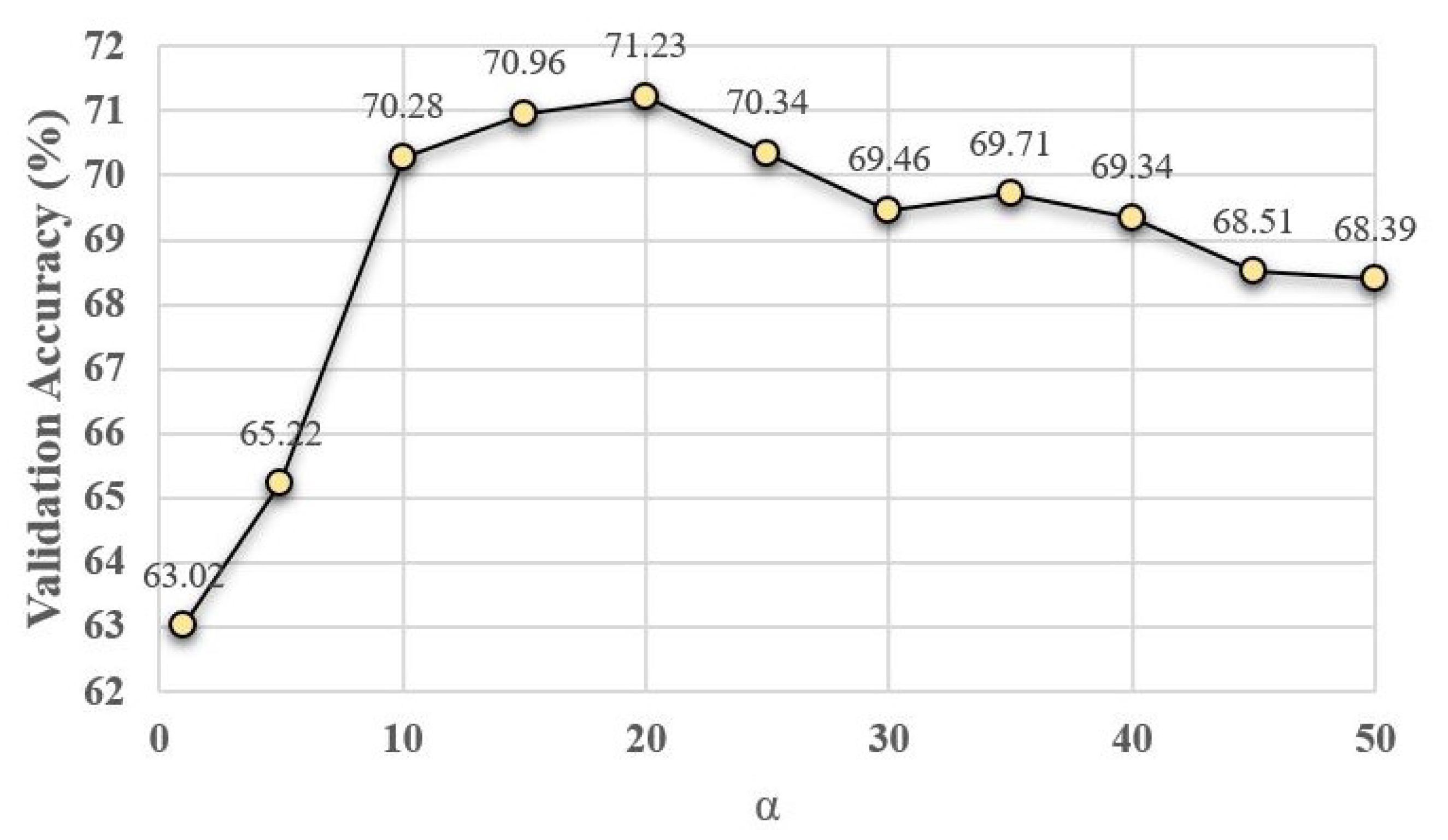
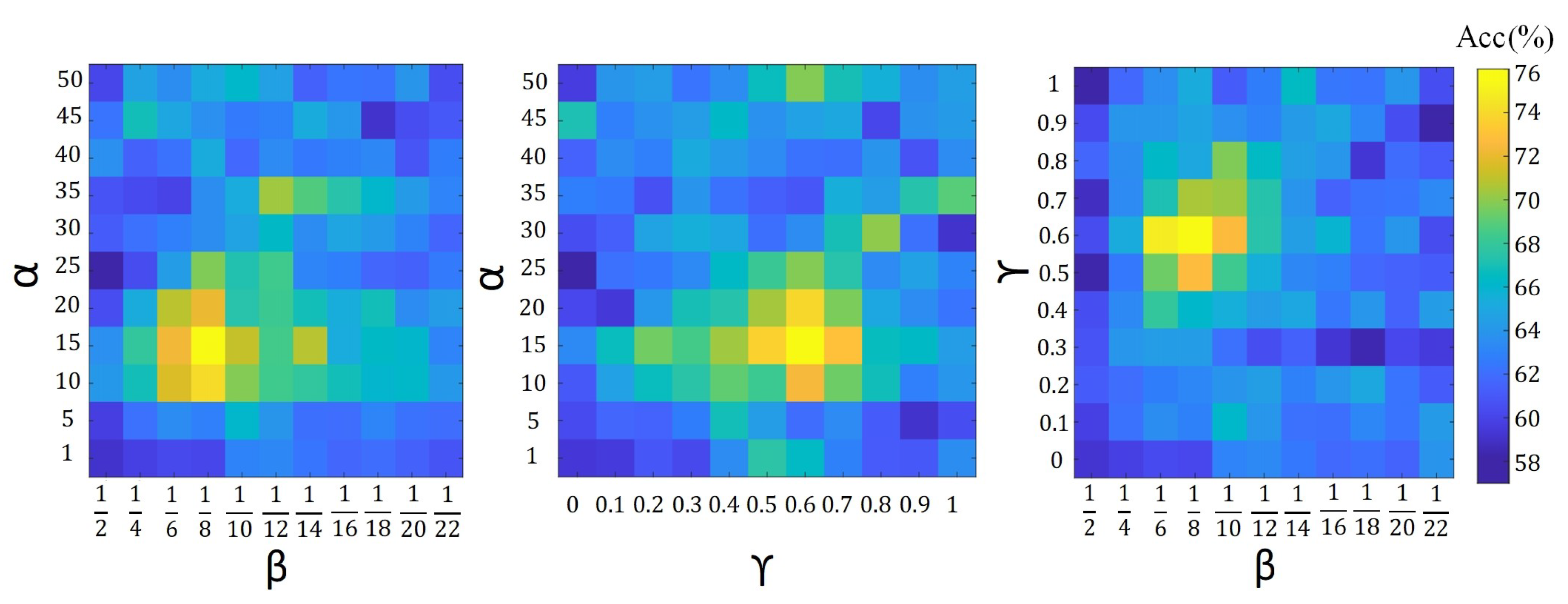
21), on the accuracy of proposed algorithms, we show the validation accuracy of their different configurations. For each setting of our search space, the model is trained on the training set and evaluated on the validation set. The configuration with the highest validation accuracy is chosen as the optimal model and further evaluated on the testing set. The validation search space for different parameter configurations is defined by
,
where
and
.
Figure 4,
Figure 5 and
Figure 6 show the average validation accuracy for all considered configurations of hyper-parameters in (
10), (
19), (
20) and (
21) on the CIFAR10 dataset. As shown in
Figure 4,
Figure 5, and
Figure 6, the optimal configurations of hyper-parameters for MI dropout, DPP dropout and DPPMI dropout are
,
, and
, respectively.
To verify the effectiveness of our proposed algorithms, we compare our approaches with recent dropout techniques, including the Automatic dropout [
17], Controlled dropout [
22], DropMI dropout [
24], Guided dropout [
15], Concrete dropout [
23], and Targeted dropout [
18], as well as the Standard dropout [
10]. All the experiments are carried out using GPU-based Tensorflow [
44] on Python 3. The simulations are processed in a system with a 10-core CPU with Intel core-i7 Processors, an NVidia Quadro RTX 6000 GPU, and a 256-GB RAM.
4.3. Numerical Results
Table 1 compares the proposed approaches’ classification performance with the referred state-of-the-art algorithms on four benchmark datasets. In line with the observations in [
40,
45], our results on CIFAR10 and CIFAR100 datasets verify the superiority of the ResNet50 over the VGG16 feature extractor backbones. Also, the obtained results verify the capability of dropout methods in overfitting mitigation [
10]. For example, by comparing the results of Standard dropout and No dropout, one can observe that with VGG16 feature extractor on CIFAR10 and CIFAR100 datasets, Standard dropout increases the test classification accuracy
and
, respectively. From comparing the obtained result between Standard dropout and Automatic dropout, we found that Automatic dropout works slightly better than the Standard dropout; for example, on the SVHN dataset, the Automatic dropout enhanced by
. The results show the same behavior in slightly better performance of Automatic dropout over Standard dropout for CIFAR10 and CIFAR100 (e.g., with ResNet50 backbone
and
improvements, respectively). The reason for this observation is the existing similarity between Automatic dropout and Standard dropout. Like Standard dropout, in Automatic dropout, the
p coefficient is considered randomly from a Gaussian probability distribution,
, but each cluster of activation functions has its own
p. Similar to [
22], the obtained results verify that Controlled dropout gained a little improvement compared to Standard dropout (e.g., with VGG16 feature extractor
and
on CIFAR10 and CIFAR100, respectively) in the neural network’s performance, despite having lower memory usage.
According to
Table 1, Guided dropout achieves higher performance across all datasets than Standard dropout, Automatic dropout, and Controlled dropout. For example, one can observe that with the VGG16 backbone, Guided dropout’s test accuracy on CIFAR10 and CIFAR100 are
and
, respectively, while these values for Controlled dropout are
and
. This enhancement in the classification accuracy is because, in contrast to previous methodologies that generally determine the
p parameter randomly, Guided dropout seeks to optimize the
p parameter; hence, picking the neurons in a more informative manner.
Concrete dropout achieves higher performance than the Standard dropout, Automatic dropout, and Controlled dropout. For instance, compared to the Controlled dropout on the SVHN and CIFAR100 datasets with ReseNet feature extractor, Concrete dropout obtains and improvements, respectively. This is because Concrete dropout finds an optimized rate for p and the model’s tunable weights with respect to the defined variational interpretation-based objective function. Moreover, one can observe the small improvement of the results by Concrete dropout over Guided dropout. With ResNet50 feature extractor on CIFAR10 and CIFAR100, the Concrete dropout test accuracies are and , while these values for Guided dropout are and , respectively. The reason for this improvement in the results is that Concrete dropout considers the unique and more advanced objective function; however, Guided dropout simply finds the neurons’ contribution based on the model’s error.
In contrast to previous approaches that deal with all NN’s neurons, by applying the dropout on the portion of neurons with low-importance connections, i.e., neurons with small , Targeted dropout with and test accuracies achieves the best results among referred baselines on MNIST and SVHN datasets, respectively. However, for more complex datasets, CIFAR10 and CIFAR100, DropMI with and on ResNet50 backbone, gains the highest accuracy in comparison with other dropout algorithms. Generally speaking, the obtained results show a similar performance of Targeted dropout and DropMI dropout. The reason for the superiority of DropMI dropout over Targeted dropout on CIFAR10 and CIFAR100 is that Targeted dropout does not consider conveying information from latent kernels to the output, while DropMI determines the important kernels by computing the MI between kernels and the target vector. This information volume plays a critical role in solving the more challenging tasks such as colored image recognition, i.e., CIFAR10 and CIFAR100.
As shown in
Table 1, the proposed DPP dropout method in
Section 3.2 that selects the diverse set of latent kernels has a better performance compared to No dropout. For example, notice the
and
improvement on the test accuracy of No dropout by DPP dropout on SVHN and CIFAR10 (with VGG16 backbone) datasets, respectively. This superiority concludes that the concept of diversity in selecting kernels must be considered in the deep latent space. Moreover, DPP dropout shows a higher test accuracy in comparison to the Standard dropout with
and
improvements on CIFAR10 and CIFAR100 respectively using ResNet50 feature extractor. The reason for this observation sheds light on the difference between random sampling and DPP sampling. However, since the DPP dropout keeps the kernels merely based on the concept of diversity in the kernel space and does not consider the importance of the kernels to the underlying task, it shows a lower test accuracy than other baselines across all datasets.
As reported in
Table 1, the proposed MI dropout with VGG16 achieves the test classification accuracy of
and
on CIFAR10 and CIFAR100, respectively. The proposed MI dropout outperforms the best mentioned dropout method on CIFAR10 and CIFAR100 (with VGG16 backbone), i.e., DropMI dropout, by
and
. This is because, in contrast to DropMI, which merely selects the kernels that include high MI with the target vector, the proposed MI dropout minimizes the shared information between selected kernels, and chooses highly relevant task-specific kernels. This superiority concludes that some kernels in the latent space of deep NNs convey similar information to their subsequent layer. Hence, choosing the set of kernels with high MI with target vector and with low MI between each other can help mitigate overfitting, i.e., increasing the test accuracy.
Furthermore, integrating MI into DPP dropout by defining a new kernel matrix and selection probability rank helps DPPMI dropout to achieve a higher test accuracy among DPP dropout, MI dropout, as well as the different referred baselines. Based on
Table 1, DPPMI dropout outperforms the best algorithms among baselines, i.e., Targeted dropout on digit recognition and DropMI on colored object recognition. The proposed DPPMI improves the accuracy of Targeted dropout by
and
on MNIST and SVHN datasets; also, it outperforms DropMI with ResNet50 backbone by
and
on CIFAR10 and CIFAR100. This observation is because the DPPMI dropout considers the diverse and most relevant kernels set to the underlying task. By comparing the obtained results among DPPMI dropout, DPP dropout, and MI dropout algorithms, one can notice that DPPMI dropout shows better performance compared to MI dropout. For instance, DPPMI dropout method with VGG16 feature extractor yields
and
improvements compared to MI dropout on CIFAR10 and CIFAR100, respectively, while in the same comparison between DPPMI dropout and DPP dropout, one can observe
and
improvement in test accuracy of DPP dropout by DPPMI dropout. This observation concludes that the concept of quality and quantity of information is more critical than selected kernels’ diversity.
4.4. DPPMI Dropout as Model Compression
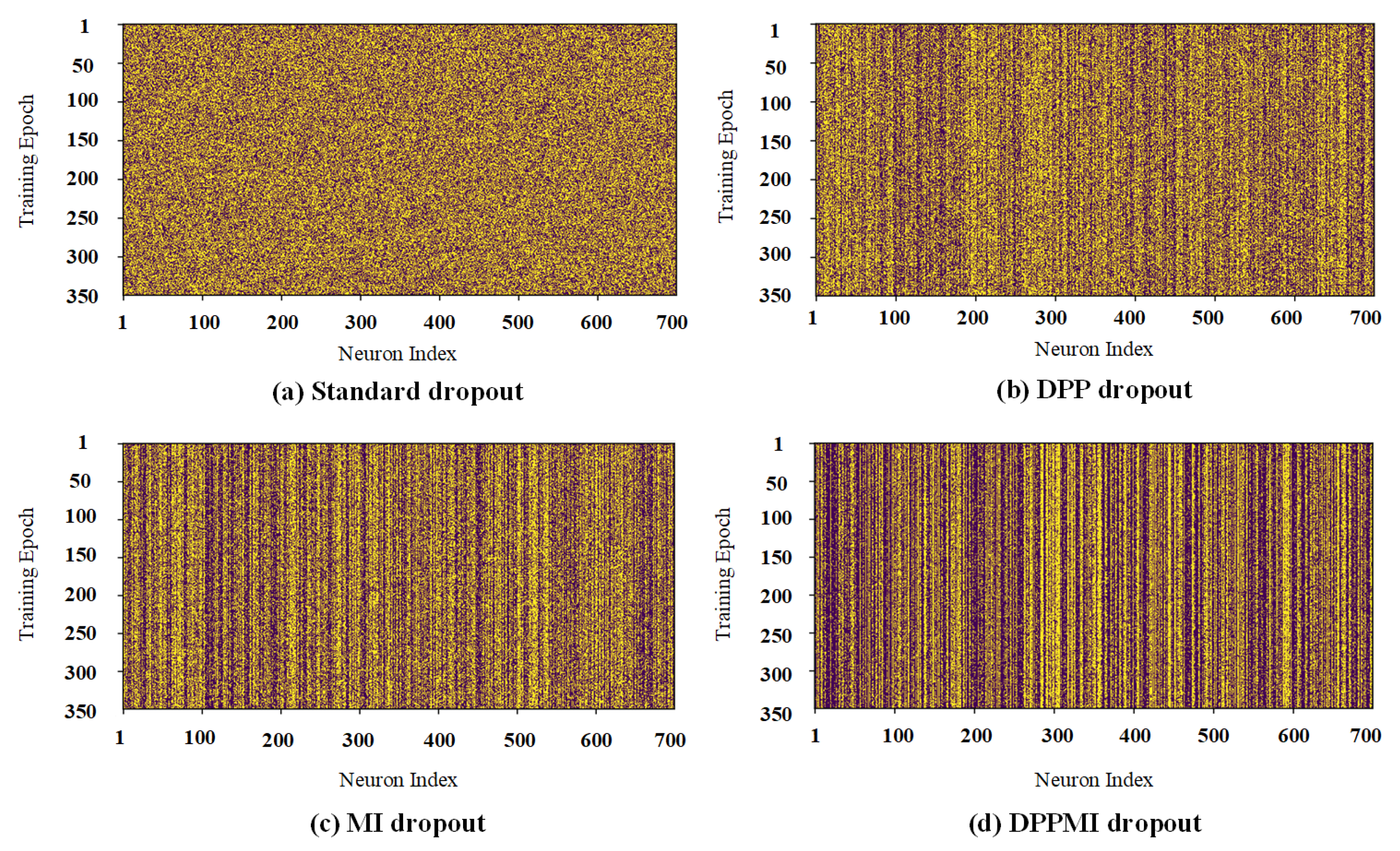
Our proposed approaches aim to avoid randomness in dropout selections and retain the neurons based on their performance in the training phase.
Figure 7 visualizes the neuron activations in the first dense hidden layer of a network trained on the CIFAR10 dataset. Each row of the visualized matrices in
Figure 7 represents the dense layer’s activation map for the entire training phase. The dark pixels show the inactive neurons, and the bright ones show the active neurons in the model. In this figure, we notice the difference in activated neurons in Standard dropout and DPP dropout. As expected, the selection in the Standard dropout is random; thus, this method gives a noisy activation map. However, DPP dropout selects the set of neurons based on the diversity criterion. Therefore, in this method, some neurons gained a higher probability rate compared to other neurons.
From the comparison corresponding to the activation maps of DPP dropout and MI dropout, one can see that MI dropout is choosing a lower number of neurons in each training epoch. At initial steps, MI dropout determines and retains the more informative neurons and updates their corresponding weights. Since MI dropout only trains the corresponding weights of the informative kernels, the probability of selecting these kernels will increase at each training step. Obviously, some neurons contribute (are active) in the underlying task for almost every training epoch; thus, they earn a lower probability of being removed. However, some neurons have less contribution in the model; hence, they gain less probability. Please note that compared to other activation maps in
Figure 7, in the DPPMI dropout’s activation map, there are more activated units because it selects neurons more strictly at each training epoch.
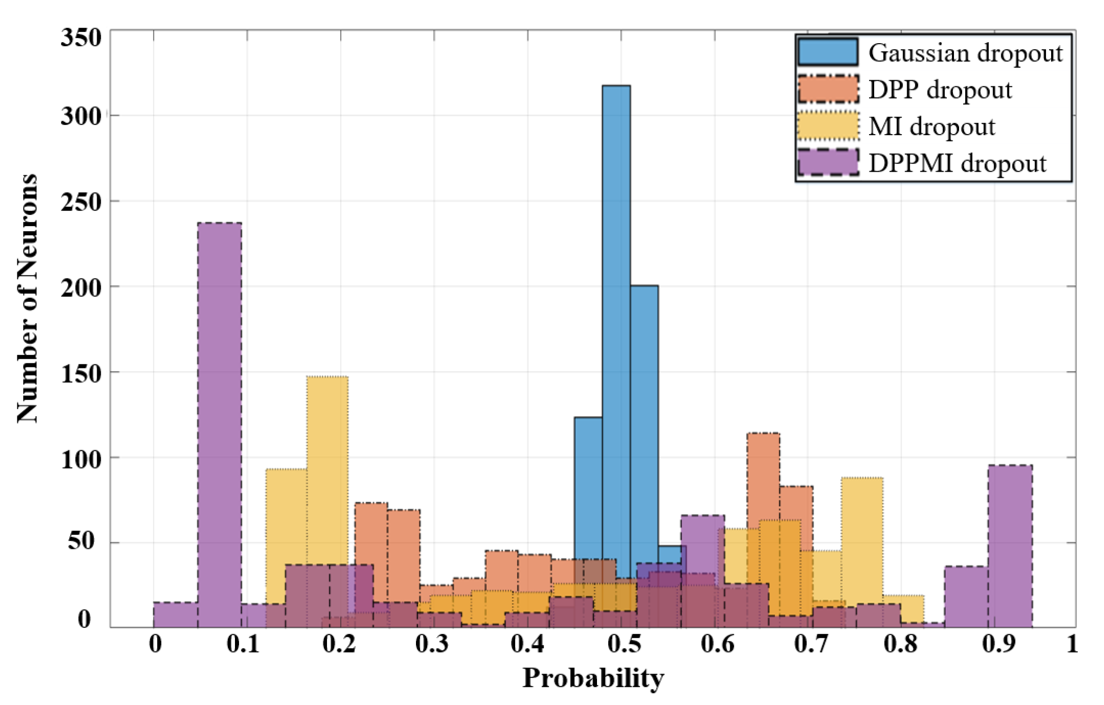
Based on the obtained masks in
Figure 7 and using (
19), we calculate the dropout probability for every single neuron in the model.
Figure 8 compares the histogram of the neurons’ probability for standard Gaussian dropout and the proposed approaches. One can observe that DPPMI dropout determines the most active neurons, i.e., the neurons that gain
, as well as the least active neurons, i.e., the neurons that earn
, in the highest and lowest probability regions of the histograms in
Figure 8, respectively. Considering this rate of contribution gives us a better sight for pruning the model. More concretely, in the case of model compression, we can prune the model by removing the set of neurons with a lower
; however, it should be emphasized that determining the threshold rate,
, depends on the dataset and the underlying task.
4.5. Discussion on Overfitting Prevention
To investigate the capability of overfitting prevention for the proposed dropout methods, similarly to [
45], we conduct two experiments. Deep neural networks encounter the overfitting issue due to having a large parameter space and a relatively low number of training examples. As mentioned in
Section 4.2, we extract the features using the VGG16 [
39] baseline. The deep visual features are fed to dense layers. In the first experiments, we increase the model’s parameters by adding some hidden fully connected layers. Thus, in each step of this experiment, we consider 2, 4, and 8 dense layers and each layer consists of 800 neurons.
Table 2 shows the numerical results of these experiments on the CIFAR10 dataset. Comparing this table’s columns, we notice that with the increase of model’s depth, the performance generally drops for all algorithms. When we compare the first and the third columns of the model on No dropout row, we see that the performance drops by
. However, this value for other baselines such as Guided dropout and Controlled dropout is less than
. This shows the importance of dropout methods to help avoid overfitting while providing high generalization capacity in very deep neural architectures. A similar analysis for the proposed DPPMI dropout and the best baseline on CIFAR10 dataset, DropMI dropout, shows that the performance declines by
and
, respectively.
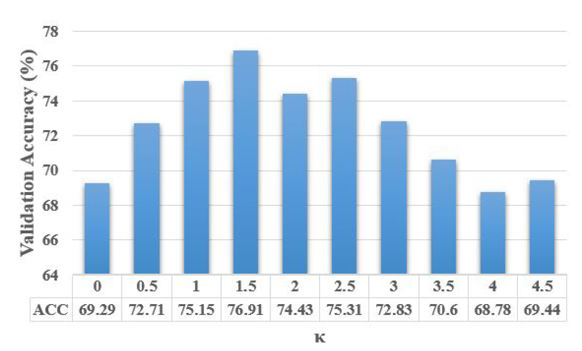
In the second experiment, during the training phase, we decrease the number of training samples uniformly for each class of the CIFAR10 dataset, while the number of hidden layers is fixed as explained in
Section 4.2. In this experiment, we defined a coefficient
that represents the relative number of training samples compared to the original size of the training data. For example, when
, for each class of the CIFAR10, we randomly choose 50,000 × 0.6 = 30,000 samples for the model’s training while the number of testing samples remains the same as the original dataset.
Table 3 shows the results of this experiment. According to this table, with the decrease in
, the test classification accuracy of the underlying model with different dropout approaches drops dramatically as expected. The gap between
and
columns for No dropout and Standard dropout is
and
, respectively. Hence, similar to the first experiment’s results, the obtained results in the second experiment reveal the role of dropout layer in model’s generalization enhancement. As shown in the table, the DPPMI dropout achieves the best performance on the three cases with different
s. In the table, we compare the results of the best baseline, i.e., DropMI dropout, and the proposed DPPMI dropout. The gap between the results of DropMI dropout for
and
is
, while the same metric for DPPMI dropout is
. Moreover, a similar analysis shows that the existing gap for MI dropout is
; therefore, the DPPMI dropout makes almost
improvement in the model’s generalization compared to proposed MI dropout. As a result, the designed experiments strongly conclude that with the increment of model parameters and the shrinkage of the training dataset, the proposed DPPMI dropout approach outperforms all recent benchmarks.
4.7. Comparison with Batch Normalization
Batch Normalization (BN) [
8] is another regularization method that aims to change the distributions of internal neurons of a deep model in training phase to reduce internal covariate shift. Whitening (normalizing to obtain zero mean and unit variance [
46]) of the inputs of each layer is the fundamental idea of BN to achieve the fixed distributions of inputs that would diminish the ill effects of the internal covariate shift and accelerate convergence of deep neural architectures [
8]. Numerous recent studies have shown that combining dropout algorithms with BN needs caution since it leads to inconsistencies in internal variance of units which causes high classification error rates during both train and test stages [
47,
48,
49].
In this section, we investigate the relationship between the proposed dropout algorithms and the BN method on training deep learning models. The experiment is carried out on SVHN and CIFAR10 datasets, and the classification baselines for these two datasets is considered similar to the explained baseline in
Section 4.2. In this experiment, we exploit ResNet50 to extract the features from CIFAR10, also the regularization methods are only applied on the dense layers in the baseline. To see the effect of variance shift between training and testing datasets, we consider two sets of configurations between the dropout and BN layers: (
A) dropout After BN layer (
B) dropout Before BN layer. All the experimental settings, i.e., number of epochs, learning rate, weight initialization, batch size, etc. are considered similar to the settings in
Section 4.2.
Table 4 compares the train/test accuracies obtained after training models with the incorporation of BN into the proposed dropout algorithms as well as the Standard dropout. By comparing the obtained results of
Table 1 and
Table 4, one can observe that the BN and Standard dropout show similar performance in terms of train and test accuracies in the training of the deep NNs. As shown in
Table 4, the (
A) configuration shows significantly better results compare to (
B), especially in the test phase. This concludes that combining these two methods, i.e., dropout and BN, does not necessarily lead to the better generalization; hence, the results verify that the covariate shift happens when there exists a BN layer after the dropout layer [
47,
50]. The whitening effect of the BN layer on the latent kernels would lead to a more uniform latent space, thus, selecting the diverse group of features would be easier for our DPP procedure. As a result, the accuracies shown in
Table 4 have consistent improvements when adding the BN layer before the dropout.


 ,
, 


