1. Introduction
In modern society and starting from this century, Unmanned Aerial Vehicles (UAVs), or drones, are widely used around the world. The recent popularity of UAVs is primarily due to the progress in developing the precision sensors, such as gyroscopes and motion sensors, which are employed to guide, navigate and control the UAVs for tracking and observation purposes in the candidate region. As a result, UAVs are fairly inexpensive and cost-effective compared with other available infrastructures, such as traditional satellite-based systems, sensing, and traditional communication systems. UAVs were first used by the military especially in the photogrammetry and 3D scanning for tracking and surveillance purposes, as in References [
1,
2,
3]. Then, different civilian applications, including UAV photogrammetry, were developed, due to their low operating altitude, which can provide a high space resolution data [
4,
5]. The relative low cost of the UAV-based systems in many areas has earned considerable success. UAVs are now used in multiple areas, including tracking, search and rescue tasks, package delivery, smart policing, video recording, and precision agriculture [
6,
7]. In view of emerging trends in UAV technologies, UAVs are expected to become an integral part in the modern technologies.
UAV complements the conventional satellite-based systems, or even replace them [
8,
9,
10]. However, the ubiquity of UAVs creates such security and privacy concerns. The massive rise for the commercial UAVs presents many problems in the fields of airspace management, and health and personal data protection, given the huge potential to promote and achieve better economic growth [
11]. In September 2017, an Army Chopper was hit by an unauthorized drone across one of the residential area [
12]. A small UAV also crashed in January 2015 in the lawn of White House and created concern about the existing safety measures [
13]. Due to their low visibility, UAVs often provide the ideal platform for illegal smugglers. For example, U.S. officials recently confiscated smuggled medicinal products by the Mexican cartels [
14], and the police in China has exposed the illicit smartphone trade from Hong Kong to the mainland of China [
15]. UAVs are also used by prisoners to move items inside and outside the prison [
16]. Moreover, they introduced more critical challenges for the public and officials due to their ability to carry high explosive payloads.
In reality, following the rules of the UAVs is not an easy task. Most UAVs still have not been registered, and other UAVs cannot have a geofencing or the geofencing option can be easily turned off. Hence, there is a huge demand to detect directly the intruder UAV in the restricted area or recognize its presence and the operating mode in the forensics investigations. The optimal detection technique should warn people if unauthorized UAVs entered the restricted area at earliest stage. Then, countermeasures can be applied on the UAV intruders and the UAV owner can be monitored and identified afterwards. Therefore, it is extremely necessary to effectively detect the consumers of UAVs. In addition to detecting UAVs, it is extremely beneficial for forensics to recognize the operating mode of the UAV. indeed, the ability to recognize the operating mode of the intruder UAV allows investigators to recover accidents that can be used as court proof in cases and enable officers to better countermeasure or respond to different potential UAV accidents. Based on different examples that were mentioned earlier, it is a prime concern to identify and remove intruding UAVs before introducing any serious problems in the infrastructure. Hence, UAV detection has become a priority in the current research directions due to the urgent need for human health, privacy and security. Academia and industry have investigated this challenge thoroughly for the commercialization of intruding UAV-based systems. The autonomous detection, monitoring, and identification of UAVs is a highly important operational key in some market systems and architectures that were suggested by researchers. In general, detection approaches work based on Radio Frequency (RF) signals [
17], RAdio Detection And Ranging (RADAR) [
18,
19,
20], acoustic [
21], Light Detection and Ranging (LiDaR) [
22], or based on cameras (passive optics), along with computer vision techniques [
23]. These detection approaches may be less successful in some realistic situations, particularly in a crowded urban environment by using only one of these sensors for detection. Radar signals may be obscured by walls and buildings and other barriers, which in urban environments are very common. Vision techniques cannot be used in the dark and Non Line-of-Sight (NLoS) scenarios for detecting the UAVs. The acoustic-based identification techniques can be interfered with the sounds of the atmosphere that might overshadow the sound created by the UAV [
17,
18,
19,
20,
21,
22,
23].
Table 1 summarizes the pros and cons of these detection techniques.
The investigation of the resulted RF signals from the UAV controllers is a promising process for detecting UAV as discussed in Reference [
24]. Indeed, the behavioral biometrics of the UAVs can be defined using Machine Learning (ML) techniques from the captured RF signals. These techniques are trained based on the raw data, which is coming from the RF signals when the UAV controller is managed by the authorized owner. In this way, numerous UAVs and the human controller on the ground can be identified. Although the biometrics compliance of the UAV operator is significant information in the detection and identification, it could be that it is little knowledge of behavioral metrics about the attacker. Therefore, the detection of the intrinsic signature of the UAV controller itself should be a priority to detect and identify any attacker UAV. Such signatures can be derived from the RF signals that are generated by the UAV controllers; it is also known as the RF fingerprints of the UAV controllers.
In general, different companies are using the UAV technology by distributing them in the sky for achieving a specific task. For security reasons, it is required to identify if there is a UAV in a specific region or not, specify the type of UAV, and the flight mode of the UAV from the radio frequency signals. Hence, this helps to identify if there is any UAV intruder in this region and decide the suitable action. In this research, we will design a simple detection approach based on the machine learning technology for detecting the presence of the UAV in known region, and then specify the type and the flight mode of the detected UAV based on the captured RF signals for that UAV. The scope of the work is detection and identification problem based on a public dataset. We designed an intelligent hierarchical approach to detect and identify the UAV, this hierarchical approach is constructed based on a set of ensemble learning classifiers. It consists of four classifiers and they are working in a hierarchical way to detect the presence of a UAV, the presence of a UAV and its type (Bebop, AR, and Phantom), and the presence of a UAV, its type, and its mode. The main contributions of this research are summarized as follows:
Review the intelligent detection and identification learning techniques in UAV technology, show the performance of these techniques in term of accuracy, complexity, advantages, and limitations.
Propose a hierarchical learning approach to solve the detection problem based on ensemble learning. In this approach, we attempt to minimize the cost of the whole approach in order to make it simple, light, and efficient.
Compare the proposed approach with other learning approaches in term of accuracy.
The remainder of this research is organized as follows. The related works are presented in
Section 2. The methodology and the system model is given in
Section 3.
Section 4 introduces the proposed detection and identification approach, and the results are given in
Section 5.
Section 6 shows a comparison between our approach and other learning approaches that use same dataset. At last,
Section 7 presents the conclusions and future works.
3. Methodology
In this section, we introduce the system model that is employed to construct the RF-UAV dataset and show the feasibility of the dataset for the UAV detection and identification problem. First, we present the system model and its components. Then, we describe the detection and identification problem. Next, we describe the structure of the RF dataset and the number of segments/samples for each case.
3.1. System Model and UAV Detection Problem
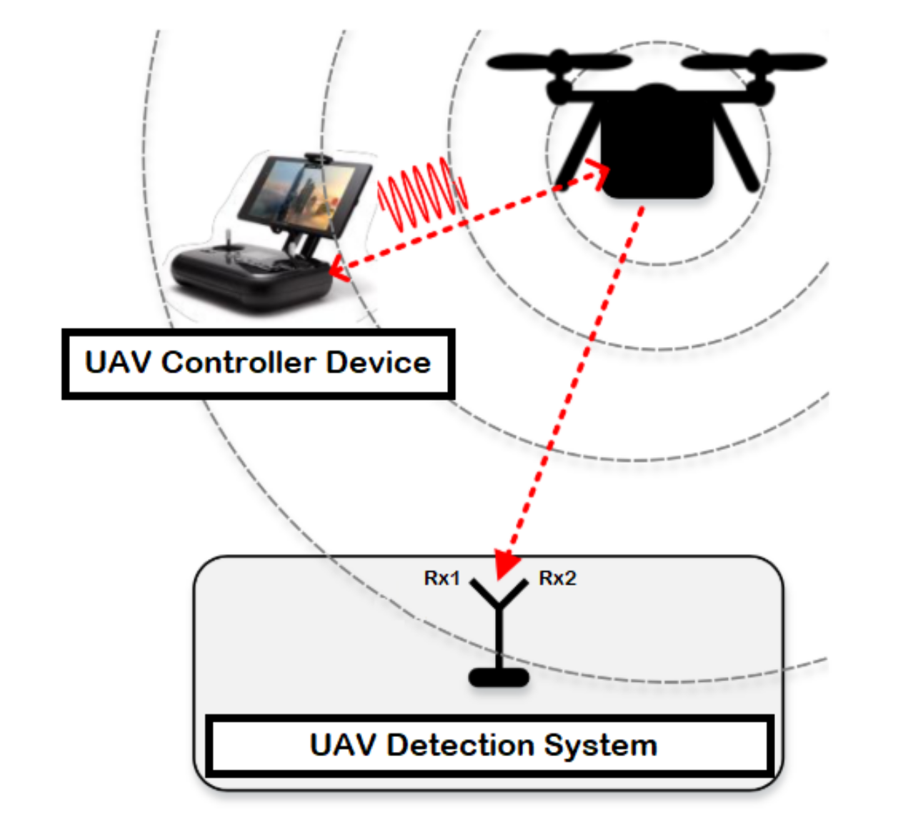
UAVs typically include on-board transmitters to control and run the UAV using only the RF signal, which are used in the communication between the UAV and the controller for data exchange purposes. These transmitter is generally works based on the 2.4 GHz Industrial, Scientific, and Medical (ISM) band. UAVs can be observed and identified from a long distance based on both the UAV itself and the characteristic of the used receiver about the surrounding environment. In addition to the benefit of employing RF signal to detect the UAVs, the used controller to transmit the signal might also be located to allow human to locate and identify the source signal.
The detection system consists of a UAV, device to control the UAV known by controller, and two receiver units for recording the received signal strength resulted from the UAV (i.e., the first one records the lower band of the RF signals, while the second receiver captures the upper band of the RF signals) as illustrated in
Figure 1. RF signals represents the communication signals between the UAV and the controller device, where the RF signals are mainly collected by employing a receiver unit (e.g., USRP-2943 40 MHz RF receiver) with an appropriate specification based on the surrounding environment as described in
Table 3. At last, the collected data is fetched, stored and processed using a laptop or any other interfacing device equipped with LabVIEW software.
In this research, we will use a public dataset, where the collected data is based on multiple experiments as discussed in Reference [
34]. The first component in the system model is the UAV, authors used three types of drones/UAVs: Parrot Bebop, Parrot AR Drone, and DJI Phantom 3. They are widely used in the research field, and each one has different specifications from the other, as described in
Table 4. The three UAVs are mainly considered as in the small UAV category due to their weights (0.4–1.2) Kgs.
The second component in the detection system model is the controller device, which represents a controlling unit that is working based on a specific application. The main goal of this application is to send/receive the main tasks to the UAV (i.e., the mode) using the RF signals. Each of the UAVs has a different application based on the developing company in order to achieve specific tasks.
The receiver unit represents the third component in the detection system; it is used to detect the RF signals from different UAVs based on the wireless communication. The main objective of this module is to detect the transmitted information in the RF form over the wireless medium. Next, this module needs to be connected with another interfacing device for fetching, analyzing, and storing the collected RF signals directly in a predefined database.
3.2. Dataset
A public dataset is used to train the proposed approach for detection and idintification the UAVs, and it is generated based on multiple experiments. The experimental system as discussed in the previous subsection contains different types of UAVs, controllers, receivers, and end user. UAVs distributed to serve a specific area with random altitudes, to study the behaviour of the received signal strength for these heterogonous UAVs. ML is used for learning the detection system based on the captured RF data. For powerful classification approaches with low variance and bias values, both quantity and quality of data were considered as important factors in the training and testing scenarios. Hence, the approach should operate based on huge quantities of data to obtain sufficient information and to improve its generalization capabilities in order to get less variance values, as well as avoid the overfitting problem. On the other hand, the dataset should cover number of cases that originate from or imitate real scenarios to reduce the bias values in the learned model, as well as avoid the underfitting effect.
In UAV classification problems, reference datasets for the different modalities are still not generally known and validated. For most, if not all, researchers obtained their own data through various methods, including laboratory experiments, simulations, and outdoor measurements. In certain cases, data collected in the laboratory, for example, are combined with a certain amount of noise to simulate a real environment. This research is based on a dataset that was generated based on a real experiment [
34]. It consists from set of recorded raw samples and segments for each class with respect to different number of experiments. The collected RF data at the receiver side is usually used for training and testing the model. The recorded time for the RF background activities is around 10.25 s, and the RF UAV communication for each flight mode is roughly around 5.25 s. The used dataset in validating our approach was published in 2019 [
34], and the recorded segments were collected based on three different levels as illustrated below:
Level 1: it represents whether a UAV is in the air or not. Hence, there are two classes to describe this level: class one: No UAV, class two: UAV.
Level 2: it shows the type of the detected UAV, when there is a UAV in the air based on Level 1. We employ three classes based on how many type of UAVs in the network and we name them based on their types: class one: Parrot Bebop, class two: Parrot AR, and class three: Phantom 3.
Level 3: it represents the flight mode of the UAV that was detected in Level 2. So, we have four modes (four classes) for each UAV (e.g., Parrot Bebop and Parrot AR):
Class One: ON (mode-1).
Class Two: Hovering (mode-2).
Class Three: Flying (mode-3).
Class Four: Recording video (mode-4).
In order to prevent memory overload, the collected RF-signals were stored as segments in a CSV-format, based on the authors in Reference [
34]. This makes loading and interpreting of the RF-UAV dataset using any compatible application simple and even easier than other formats.
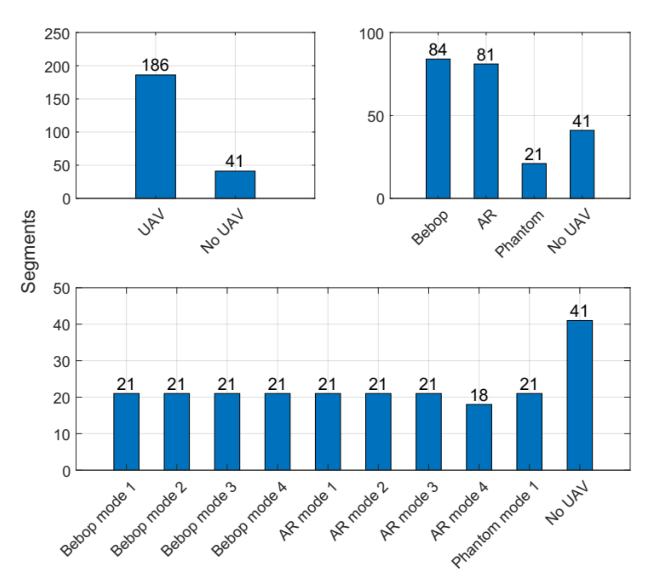
Figure 2 shows in details the recorded segments for each experimental level in the RF-UAV dataset. The dataset contains in total 227 segments, and each segment consists of 20 million samples; hence, this makes the dataset in range of a huge dataset. This dataset has been used in previous research studies [
26,
28,
32], and the distribution of samples for all cases is as follows:
Bebop UAV: 84 segments (84 × 20 × 106 samples).
AR UAV: 81 segments (81 × 20 × 106 samples).
Phantom UAV: 21 segments (21 × 20 × 106 samples).
No UAV: 41 segments (41 × 20 × 106 samples).
Based on the above description of the dataset [
34], the detection problem can be solved as a multi class problem in a hierarchical manner. From our understanding, the system will be built based on four classifiers to identify the presence of the UAV, type of the UAV, and the mode of the UAV as discussed in the next section.
4. Proposed Detection Approach
Based on the problem description, we propose an intelligent approach to classify each stage correctly, taking into our consideration the overall accuracy of all stages, as well as the simplicity of our approach. The first stage is the problem formulation, which mainly consists of specifying the system model and the collected data from the model in order to be investigated and analyzed in the next stages. UAV detection is a multi-class classification problem, and we consider some approaches in our design that have shown a good performance in multi-class classification scenarios. Stage two represents the pre-processing elements that are required to clean, transform, smooth, and normalize the collected data to be used in the next stages. Stage three represents the construction of our approach, where the learning approach is designed to solve this multi-class classification problem using different learning methods in a hierarchical manner. The last stage shows the evaluation process in term of different performance metrics. A lot of strategies and assumptions throughout the model construction and the data analysis stages are used to improve the performance of the detection system. This ML approach is built based on Scikit-learn libraries in Python 3 [
35].
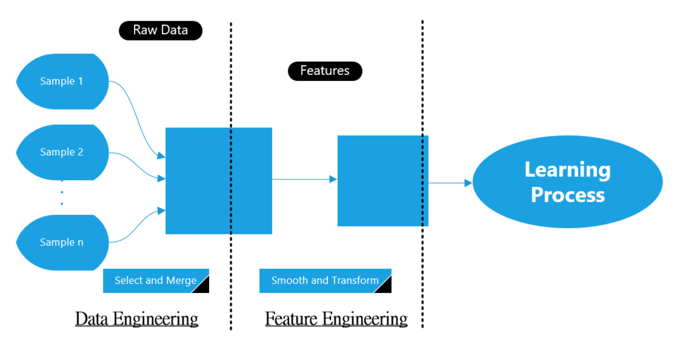
4.1. Data Pre-Processing Stage
Raw RF data in the main dataset was collected using on-board sensing units, which requires to be pre-processed again before entering the learning approach. This includes the filtering process that uses to eliminate the noises and conflict, or using various techniques to shrink the size of the data. The data pre-processing stage in ML approach consists of two units: data engineering and feature engineering. The data engineering represents how to convert the RF data from raw shape to a form to be used later on, while the feature engineering represents how to tune the resulted data from the data engineering in order to construct the features desired by the learning approach.
Figure 3 shows the typical block diagram of this stage.
In reality, methods from both signal processing and ML can often be combined to increase the predictability of the model. In our scenario, a filtering stage is applied to the input samples for smoothing purposes and reducing the noise value. This filtering stage is based on averaging concept with a predefined window. It basically does the averaging by adding N-adjacent samples and then dividing the sum by N value. Next, it directly writes the values into the Nth sample position. In general, this method represents a Finite Impulse Response (FIR) filter of a specific number of taps (N) with a uniform weighting option. Finally, smoothed values enter the learning approach in order to be classified based on a given target values.
4.2. Binary/Multi-Class Classification Stages
Classification concept is one of the supervised ML techniques, where used samples in the training and testing processes are labeled. The number of labels for a certain dataset is the same as the number of classes. The identification and detection of UAV using ML is considered as a binary classification problem, in which there are only two labels (“UAV” and “No UAV”). The detection of UAVs from birds and UAVs from other aircrafts is also cosidered as a binary classification problem with the respective data labels. In our case, multi-class problem refers to different classes and labels as we have different types of UAVs and different fight modes.
In multi-class scenarios, each training instance classifies into one class from a set of classes. The objective is to extract a feature that correctly predicts the class to which the new point belongs in view of a new data point. There are different methods that can be used to solve the multi-class problem by deploying a set of binary classifiers. One way to do that is by constructing a classification system that can classify the raw data to ten classes (from 1 to 10) by deploying a 10 binary classifiers for each collection of data. Next, if you choose to classify a certain data point, you will obtain each classifier’s decision score for that point and select the class based on the highest classification score. This solution is known by one-versus-all strategy or one-versus-the-rest. One-versus-all strategy operates by training a binary classifier for data and then matches each classifier to each input to decide the class to which input belongs to. The steps of this strategy can be described as follows:
Since we have a multiclass classification problem with N classes (2, 3, and 4), the one-versus-all strategy transforms the training dataset into some N binary classification problems.
For each class, allocate negative dataset to the input from other classes and allocate the positive dataset for the selected class. Then, we need to train this approach using a specific classifier to fit the binary dataset.
After doing the training of these binary classifiers for each class, we need to specify every input that belongs to the selected class, if its hypothesis returns the highest score with respect to other classifiers.
Using the above strategy in our approach, classifying the class based on other classes, will enhance the classification accuracy for each of the following sub-classifiers in our hierarchical learning approach:
Classifier 1 (Presence of the UAV): two classes (UAV and No UAV); it is used to specify if there is a UAV or not.
Classifier 2 (Type of the UAV): three classes after detecting the presence of the UAV from the first classifier (Bebop, AR, and Phantom); it represents the presence of the UAV and the type of the detected UAV.
Classifier 3 (Modes of the Bebop UAV): four classes after detecting the type of the UAV (four flight modes for Bebop: on, hovering, flying, flying with video recording); it is used to define the presence of the UAV, the type of the detected UAV, and the flight mode of the UAV.
Classifier 4 (Modes of the AR UAV): four classes after detecting the type of the UAV (four flight modes for AR: on, hovering, flying, flying with video recording); it is used to define the presence of the UAV, the type of the detected UAV, and the flight mode of the UAV.
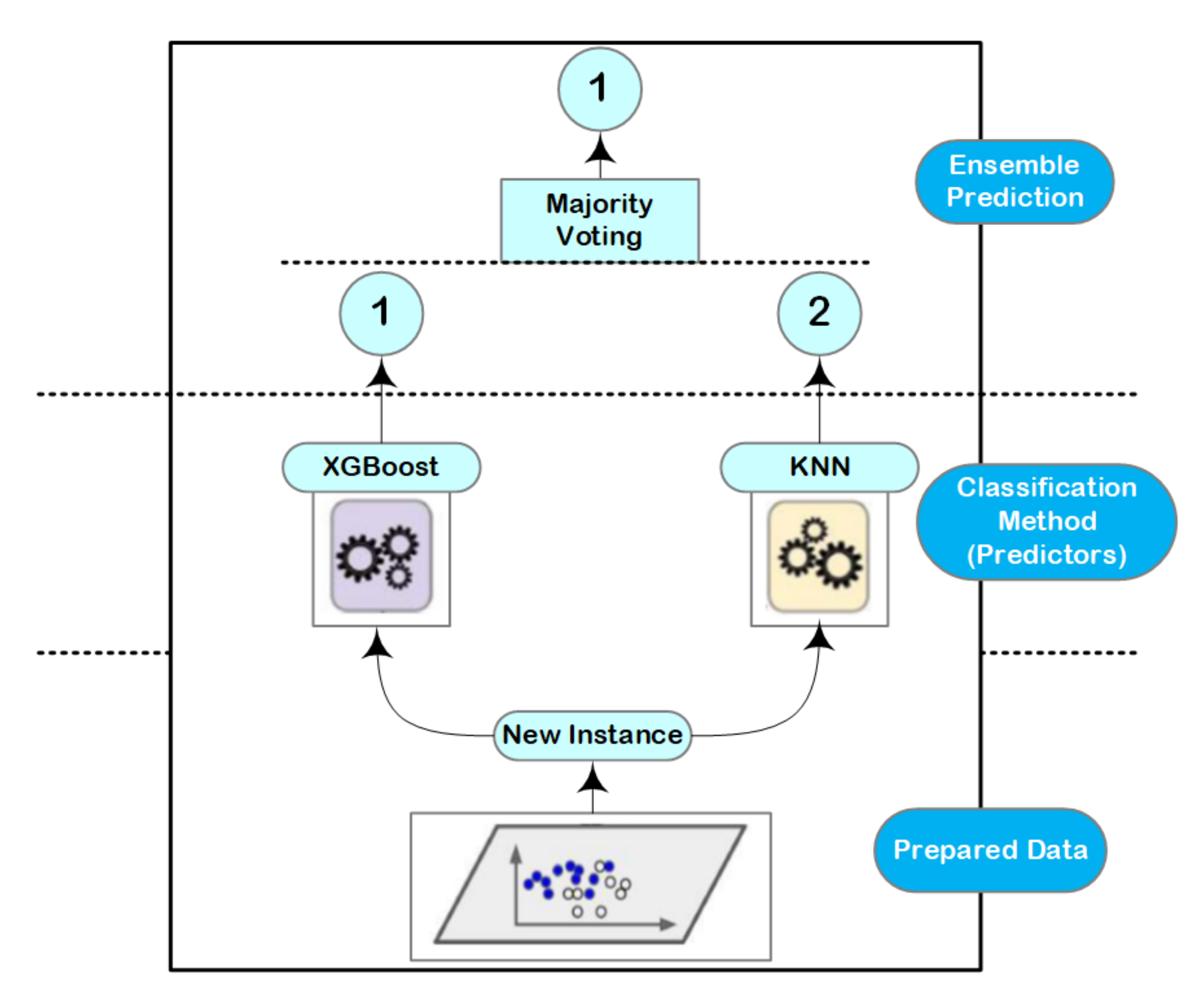
4.3. Ensemble Learning
Ensemble learning with decision trees concept is typically one of the highest performing approaches in case of a classification problems [
36]. It basically combines different classifiers into one classifier for solving a classification problem and the final score can be selected based on the majority voting principle [
37]. This voting process achieves better accuracy values compared with the best classifier in the ensemble learning as illustrated in
Figure 4. Indeed, ensemble learning approach can be a strong learner even it combines multiple weak learners, given that these weak learners are sufficiently diverse.
However, the main causes of the variations between the predicted and true values are resulted from noise, bias, and variance. In our research, it can be seen that the approach is going to either overfitting or underfitting due to these factors. Using the ensemble learning helps to minimize these errors except the irreducible error (e.g., caused by noise). That is why the ensemble learning comes into the picture directly to be used in our design. The used algorithms in our approach are: XGBoost and K-Nearest Neighbor (KNN). These algorithms are suitable and can achieve better accuracy in case of multiclass scenarios. The final score of these algorithms are selected based on the majority voting of the results.
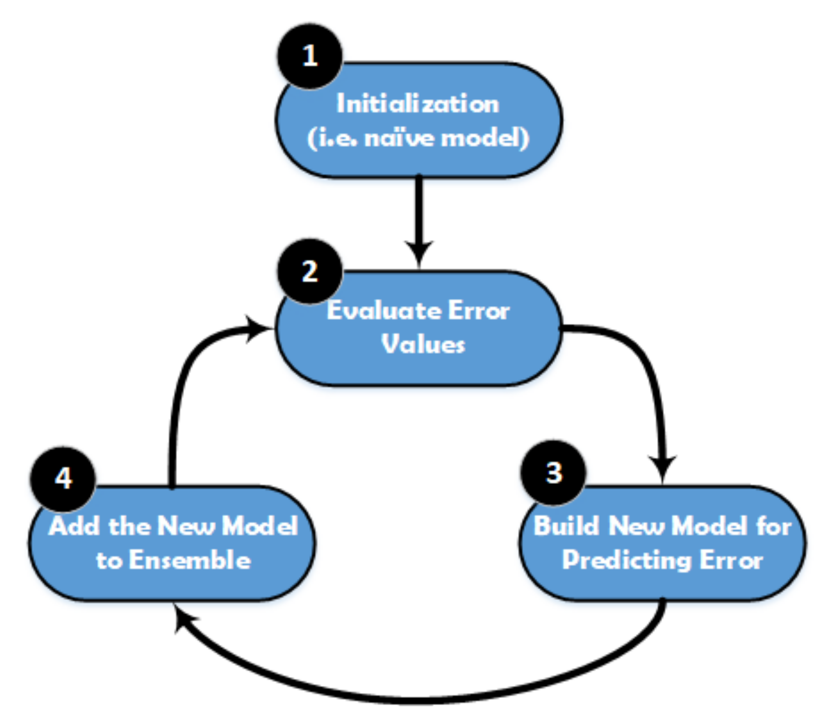
XGBoost is a popular implementation of gradient boosting, and it works based on the Gradient Boosted Decision Tree model. The main steps of XGBoost method are illustrated in
Figure 5. This model is initialized by using a simple base prediction, which handles the initialization of the first predictions. After that, it starts evaluating the error values for each sample in the dataset. Next, a new model is built to predict the samples based on the error values. The output predictions from the new model will be added to the ensemble of models. To predict any sample, we need to add all the predictions from the previous models and then use them to evaluate the new error value, construct a new model, and add it to the ensemble of models and so on. Some important characteristics can be achieved by using XGBoost method, especially when the dataset is large, such as regularization, cache awareness, parallel learning, and less number of splits in the trees, and the overfitting can be avoided by using a suitable stopping method for the boosting, and it has a positive impact on the out-of-core computing.
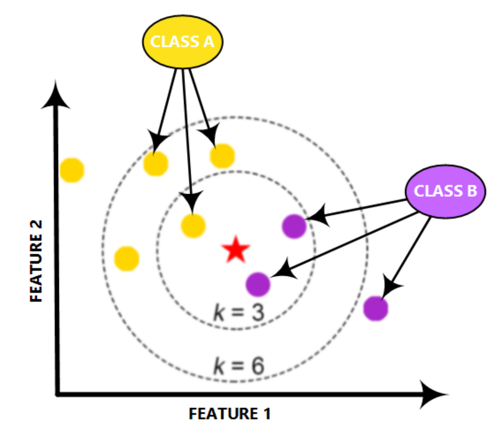
The KNN is a powerful classifier; it is said that, for a specific value of K, the KNN algorithm finds the K nearest neighbors for a given data sample, and, next, it specifies the applicable class to this sample by choosing a class which achieves the highest number of samples out of all other classes of K neighbors, as illustrated in
Figure 6.
The detection and classification problem can be solved easily in a hierarchical manner since the dataset contains RF records for a set of UAVs describing their availability, type, and mode. The hierarchical model starts by determining the availability of the UAV, and then it will specify the type of the UAV based on the detected RF signal. Once the type is defined, the mode can then be specified using the same RF signal. Therefore, it is easy to handle any sample using the hierarchical way with minimum error rate compared to a non-hierarchical approach, which warrants a need to remove the unwanted classes at each step of the classification process. The hierarchical approach minimizes the similarity of the RF signal for the detected UAVs at different classification stages. The approach consists a set of classifiers that uses the same learning process with different number of output classes (i.e., 2, 3, and 4). Each classifier works based on the ensemble learning; it is one of the best ML models that can achieve better perdition values for a set of learning techniques. Basically, the use of ensemble learning offers a systematic solution and brings a distributed model to a ML model, which helps in refining the prediction results and ensuring better accuracy. Moreover, it is an effective approach to deal with overfitting, where the model does well on the training set but fails to generalize on the test set. Since the dataset contains samples having high similarity to each other in terms of the distribution of RF signals, it is required to use a learning technique that will minimize the variance component of the prediction errors. Hence, ensemble learning is used to implement this model. It is a simple and light model, requires less processing time, and enables to find the optimal values that might reduce the variance in the RF signal with minimal processing time.
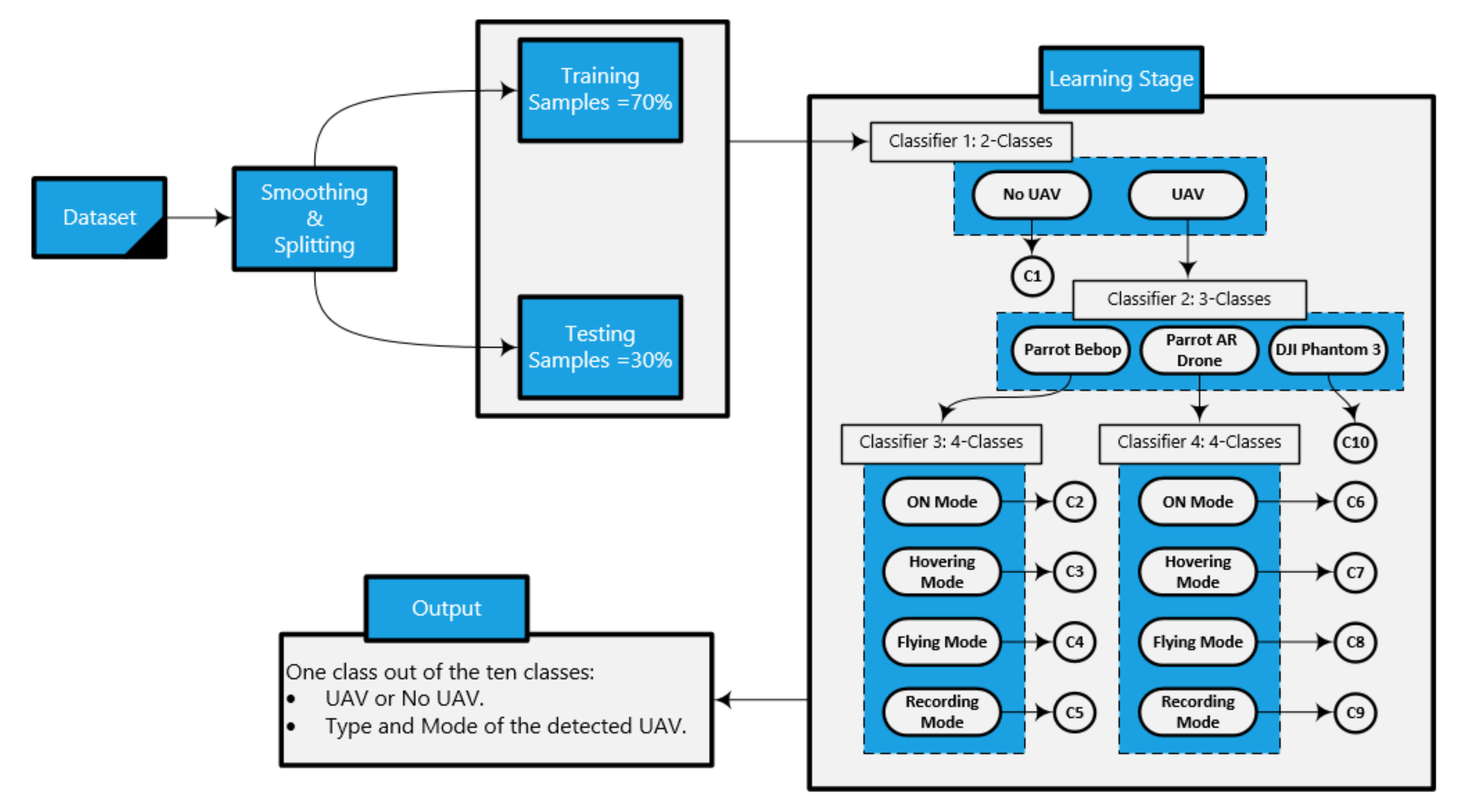
Our approach is illustrated in
Figure 7, and, in Algorithm 1, the smoothed RF testing sample enters the first classifier (binary classifier) in the learning stage. The output of this classifier with respect to our RF sample informs if there is a UAV in the detected region or no UAV. If there is a UAV in the region, this sample enters the second classifier in order to define the type of the detected UAV (Bebop, AR, and Phantom 3). If the detected UAV is Phantom 3, the output of the detection approach is class number 10. Otherwise, the testing sample enters either the third classifier, and the detected UAV is
Bebop, or the fourth classifier, when the detected UAV is
AR. The third and fourth classifiers define the mode of the detected UAV as one of the following modes based on four classes problem: on, hovering, flying, and video recording, where the classes for the Bebop UAV are: 2 for ON mode, 3 for Hovering mode, 4 for Flying mode, and 5 for Video recording mode. On the other hand, for AR UAV, the modes are as follows: 6 for ON mode, 7 for Hovering mode, 8 for Flying mode, and 9 for Video recording mode. Each classifier works based on the ensemble concept, where the constituent model consists of XGBoost and KNN. The final output is based on the voting of the outputs from the two algorithms. These algorithms are used from the Scikit-learn libraries in Python 3, and we set the best parameters for both algorithms using the grid search model in order to achieve the best accuracy for the whole detection system.
| Algorithm 1 Hierarchical learning approach. |
- 1:
Load RF dataset - 2:
Define the inputs and the outputs - 3:
Pre-process the data - 4:
Encoding the outputs with respect to the inputs - 5:
Split the data into : training (70%) and testing (30%) sets - 6:
Define the input variables and find the optimal parameters using - 7:
Records - 8:
Train the system on by calling procedure - 9:
Test the system by using and evaluate the required metrics - 10:
- 11:
procedureClassifier() - 12:
Use the optimal parameters for KNN and XGBoost - 13:
Use ensemble learning based on KNN and XGBoost - 14:
Train and fit the classifier using - 15:
Predict the test samples - 16:
end procedure - 17:
- 18:
procedureHierarchicalApproach() - 19:
from will pass the first to specify the availability of the UAV (2 classes: 0-No UAV, 1-UAV) - 20:
if then - 21:
- 22:
go to end procedure and return the predicted class () - 23:
else - 24:
will pass the second to specify the type of the UAV (3 classes: 0-Bebop UAV, 1-AR UAV, 2-Phantom3 UAV) - 25:
if then - 26:
- 27:
go to end procedure and return the predicted class: Phantom3 UAV () - 28:
else - 29:
if then - 30:
will pass the third to specify the mode of the Bebop UAV (4 classes: 0-ON (), 1-Hovering (), 2-Flying (), 3-Recording ()) - 31:
if then - 32:
- 33:
go to end procedure and return the predicted class: Bebop UAV with ON mode () - 34:
else if then - 35:
- 36:
go to end procedure and return the predicted class: Bebop UAV with Hovering mode () - 37:
else if then - 38:
- 39:
go to end procedure and return the predicted class: Bebop UAV with Flying mode () - 40:
else - 41:
- 42:
go to end procedure and return the predicted class: Bebop UAV with Recording mode () - 43:
end if - 44:
else - 45:
will pass the fourth to specify the mode of the AR UAV
(4 classes: 0-ON (), 1-Hovering (), 2-Flying (), 3-Recording ()) - 46:
if then - 47:
- 48:
go to end procedure and return the predicted class: AR UAV with ON mode () - 49:
else if then - 50:
- 51:
go to end procedure and return the predicted class: AR UAV with Hovering mode () - 52:
else if then - 53:
- 54:
go to end procedure and return the predicted class: AR UAV with Flying mode () - 55:
else - 56:
- 57:
go to end procedure and return the predicted class: AR UAV with Recording mode () - 58:
end if - 59:
end if - 60:
end if - 61:
end if - 62:
Return predicted class () and processing time () - 63:
end procedure
|
5. Results and Discussions
This section presents the results of the developed UAV detection and identification approach. First, we present the pre-processing tasks to get a cleaned data, which is suitable to be used in the learning approach directly. Next, we show the representation of the RF data in time and frequency domain for some of the selected UAV modes. Then, we show and discuss the results of our approach for the 10-classes scenario with respect to our smoothed RF data. Finally, we compare our results with other papers that used same dataset in case of 10 classes.
5.1. Pre-Processing Stage
Our selected dataset [
34] consists of around 227 segments of the recorded RF signals during multiple experiments. Each experiment was conducted using three type of drones/UAVs (Bebop, AR, and Phantom 3). The collected RF records contain around 10.25 s of RF background data when the UAVs are off and 5.25 s of UAVs communication RF data. Data was also recorded for different flight modes: on, hovering, only flying, and flying with video recording. The three UAVs was controlled by using a flight controllers based on their companies. However, two RF receivers (NI-USRP 2943R RF) were used for detection the RF signals that are coming from the UAVs, and both receivers are directly connected to laptop. The first one records the lower band of the RF signal, and the second one is for detecting the upper band of the RF signal. Authors in Reference [
34] used the two RF receivers with a maximum instantaneous bandwidth of 40 MHz that are working simultaneously to at least record part of the spectrum as in WiFi with 80 MHz bandwidth. The exact bandwidth of 2.4 GHz-WiFi is equal to 94 MHz + 3 MHz, and the second term is used as guard bands at the start and the end. So, authors did not record the first and last 1-MHz and the last channel since they contain negligible information in addition to high noises and interferences. Therefore, the dataset has almost clean RF signals based on this strategy. Hence, we used this dataset and added the filtering stage to overcome/minimize the effect of the interferences caused by high density RF signals.
The collected RF data are pre-processed by means of removing the noise for each RF signal using a smoothing filter with window equal to 15. Hence, results define that the RF signals are improved, and noises and clutters are minimized, based on reducing the variation for each data sample to be smoother than the original RF data. Furthermore, this dataset has been segmented into smaller number of segments to ensure better performance in the learning process, and these segments were represented by the Fast Fourier Transform (FFT) using MATLAB commands. Indeed, the FFT was done with zero mean signals by removing the zero frequency parts. This decreases the overall process’ computational complexity. Moreover, this stage is critical specially when the RF signals are weak in the presence of the noise and omitting the bias effect in the signals leads directly to better detection accuracy.
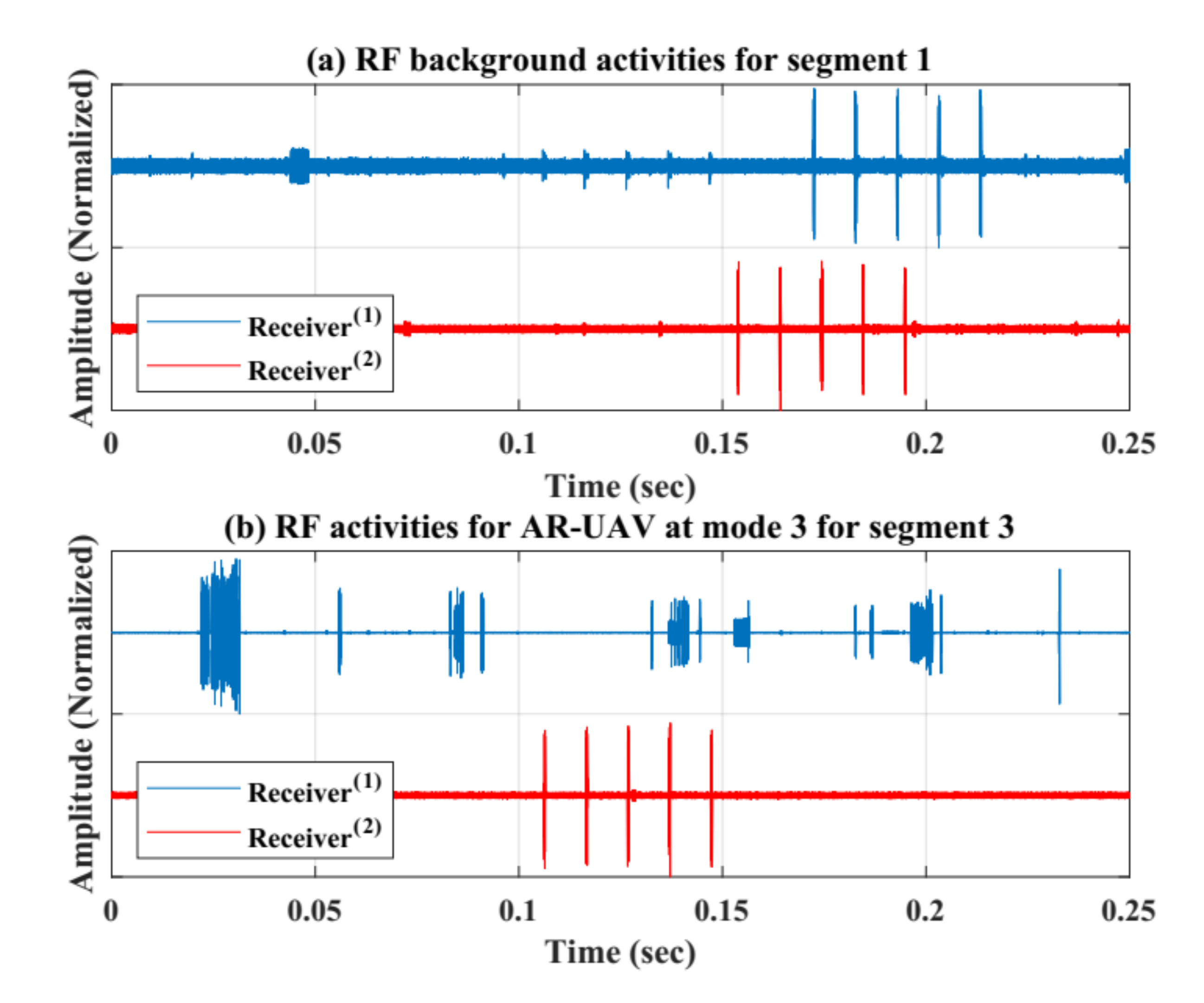
Figure 8 shows the collected RF signals using two receivers units for two segments after doing the normalization (between 1 and −1 values). (a) presents the normal RF activities for segment 1, while (b) presents the RF activities when there is a AR UAV only flying in the region without recording videos using segment 3.
5.2. Analysis of RF Dataset
The main challenge here is to extract the important information from the generated data to use them as predictor in the learning process. This part identifies the main features that are considered and chosen as inputs and the explanations behind using these features in the learning approach.
Figure 2 shows the specifications of the RF dataset and how many segments (=20 million samples per segment) for each class. It is shown in the same figure that each class has different number of segments/samples, and we divided our dataset into 70% for training process and 30% for testing process. The spectrum signals of the three given scenarios in the dataset (2, 4, and 10 classes) are shown in
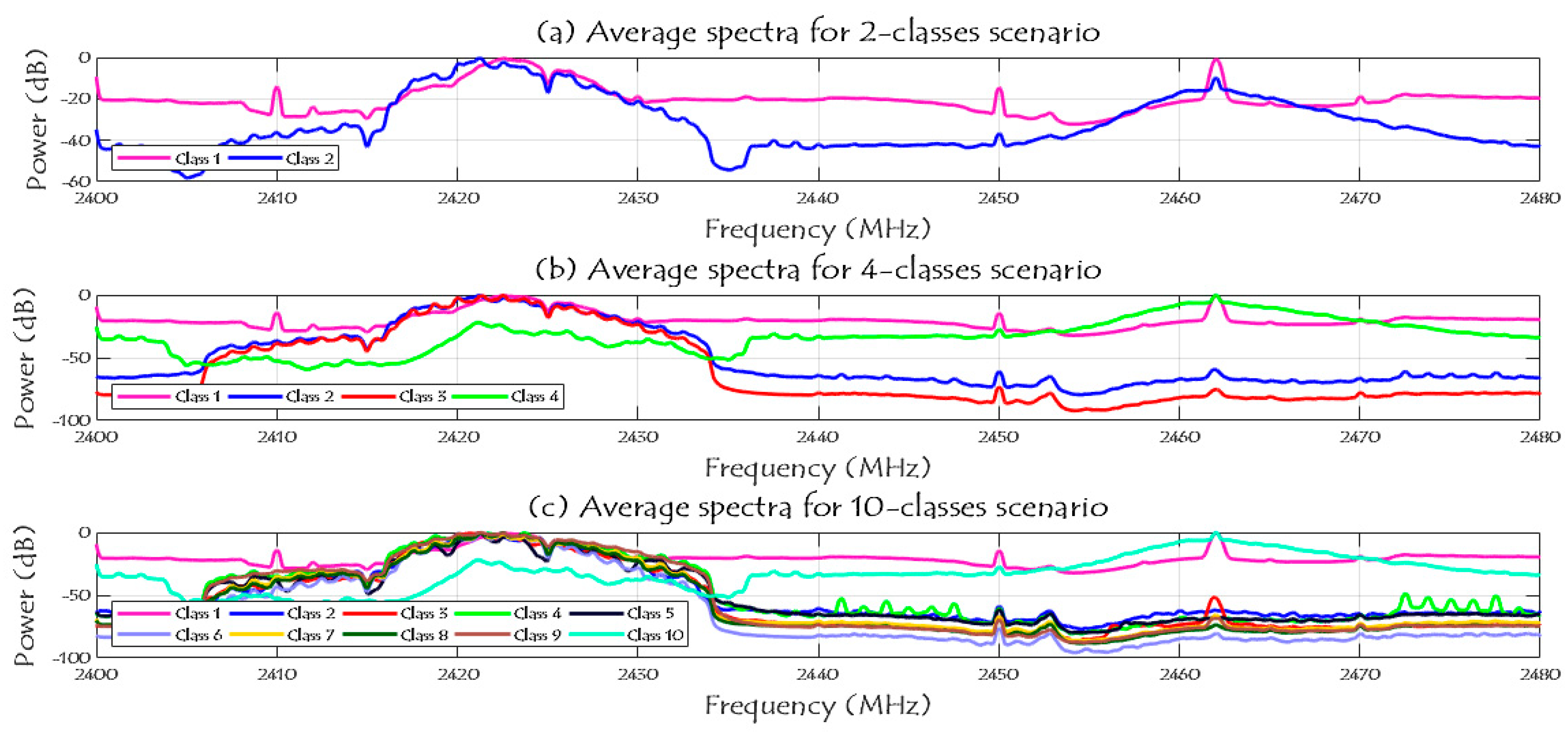
Figure 9 after reducing the noise variations and smooth the RF signals.
Note that, in case of two classes scenario, class 1 represents the RF background activities for no UAV case and class 2 represents the RF signals when there is a UAV. In case of four classes scenario, class 1 represents the RF background activities for no UAV case, and classes from 2 to 4 are for the Bebop, AR, and Phantom UAVs. In case of ten classes, class 1 represents the RF background activities for no UAV case, classes from 2 to 5 represents the flight modes of the Bebop 4, classes from 6 to 9 represents the flight modes of the AR 4, and, finally, class 10 represents the flight mode of the Phantom UAV.
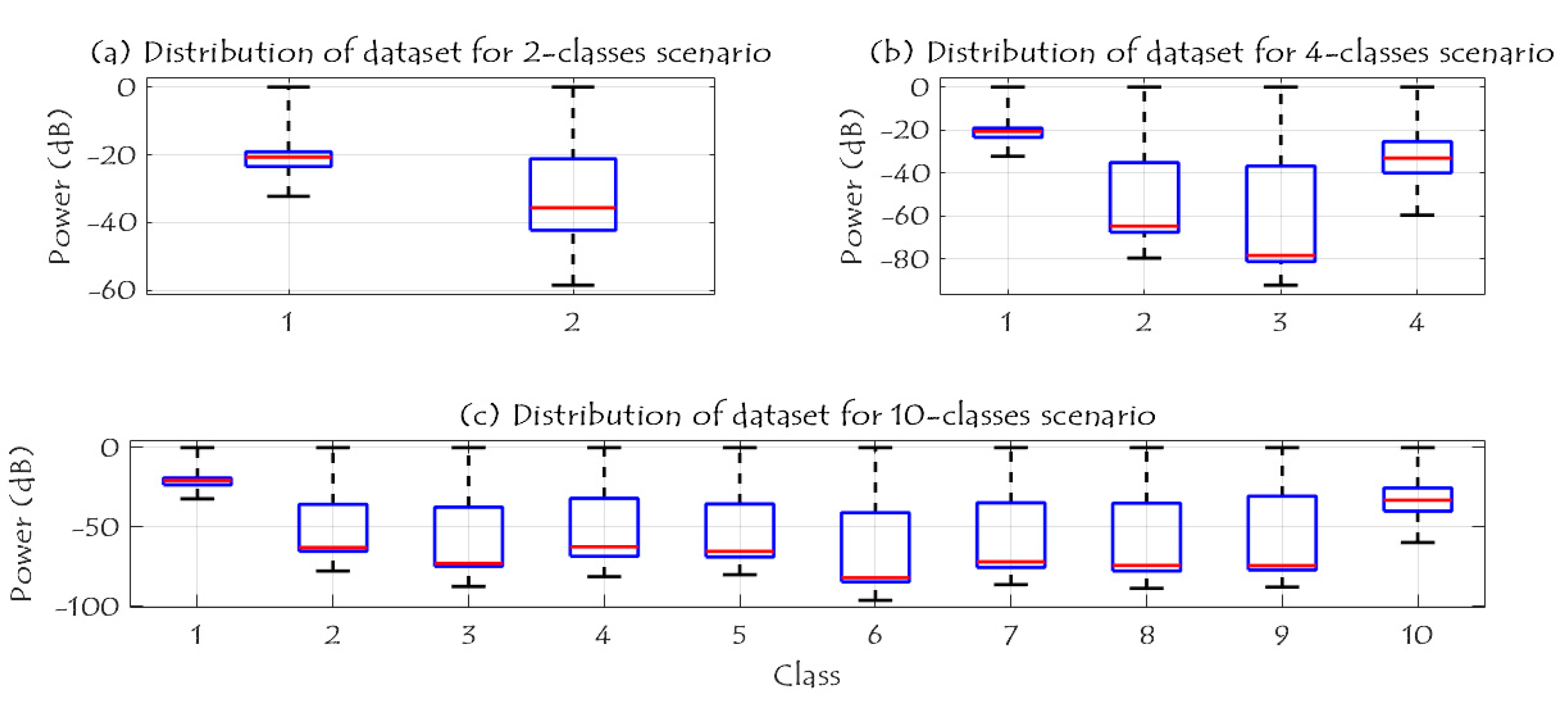
Figure 10 shows the RF data distribution of 2-classes, 4-classes, and 10-classes scenarios. Based on (a), the data distribution of the two classes (UAV and No UAV) can be easily used to identify the availability of the UAV in a specific region. Furthermore, when the number of classes has increased to four classes, the complexity of the detection problem is increased due to the same RF range for class 2 and class 3 as illustrated in (b); these two classes are the Bebop and AR UAVs that made by the same company, while class 1 and 4 can be easily identified since they are transmitted using different RF values. In case of 10 classes, class 1 and class 10 can be easily detected, while it is difficult to identify class 2 to class 5 since they have the same range of RF values for Bebop 4 flight modes, and the same thing for class 6 to class 9.
5.3. UAV Detection and Identification
The easiest way to test any detection system is by measuring the overall accuracy. However, in a situation where classes are not equally relevant to classify or when classes are imbalanced, accuracy can be a misleading option. Hence, the ratios of positive or negative being incorrect or correct are also more helpful in the evaluation. There are other metrics that might use to measure the performance of the UAV detection system, such as recall, error, precision, false negative rate (FNR), false discovery rate (FDR), and F1 scores. These metrics can be evaluated based on the following equations:
where TP, FN, and FP represent the number of true positives, false negatives, and false positives [
38]. These metrics can be evaluated and summarized in a matrix form called confusion matrix.
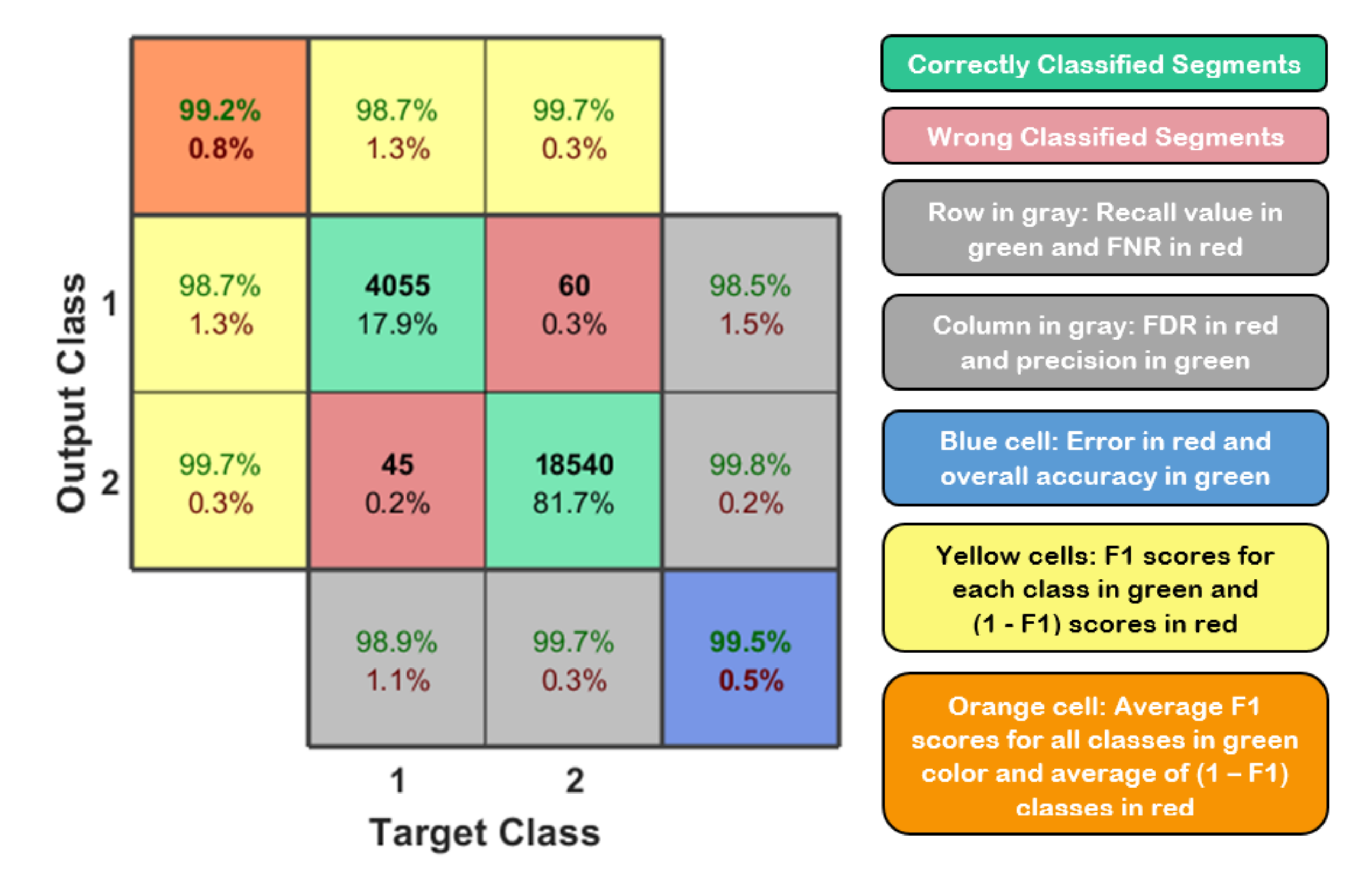
Figure 11 shows the typical confusion matrix for binary classification problem that can be generated and visualized using the output of a python 3 script and MATLAB code.
So, many performance metrics are needed to be considered when evaluating the proposed approach in order to correctly describe the overall performance of the detection and identification system. In this research, we mentioned the best evaluation metrics that need to be taken into account in the evaluation process for our learning approach. Performance evaluation of the learning approach is illustrated and summarized in the below confusion matrix for the 10 classes scenario. As discussed before, we solved our detection problem in Hierarchical manner using four classifiers (classifier with 2-classes, classifier with 3-classes, and two classifiers with 4-classes). Each classifier works based on ensemble concept using KNN and XGBoost classifiers. The reasons behind using these classifiers is that they are supporting regularization, flexibility, and built-in cross validation. Both classifiers have a set of hyper-parameters that need to be tuned to achieve better performance. The tuning process is done once in our model using “Grid Search with cross validation (cv = 3)”, and the output parameters of both methods are: for XGBoost (learning rate = 0.1, number of estimators = 100) and for KNN (K = 1) and we used the default values for other hyper-parameters [
39]. In general, the selection of these values will affect the overall output of the ensemble learning, thereby influencing the accuracy in addition to other evaluation metrics. We used the optimal values to avoid the overfitting and underfitting problems caused by setting wrong hyper-parameters. Another performance metric can be used in evaluating the learning approach is the processing time. It represents the minimum required time for the system to correctly detect the sample. It depends on the shape and the size of the dataset, as well as the machine that will handle the detection and identification process. We can consider it as the testing time of our approach, which represented based on our simulation for all samples between 6.54 msec and 7.41 msec in all scenarios.
The RF dataset has 2048 features which are fed into a hierarchical learning approach for classification. These features represent the lower and upper bands of the RF signals that collected using two receivers as explained before and in the experiment setup of Reference [
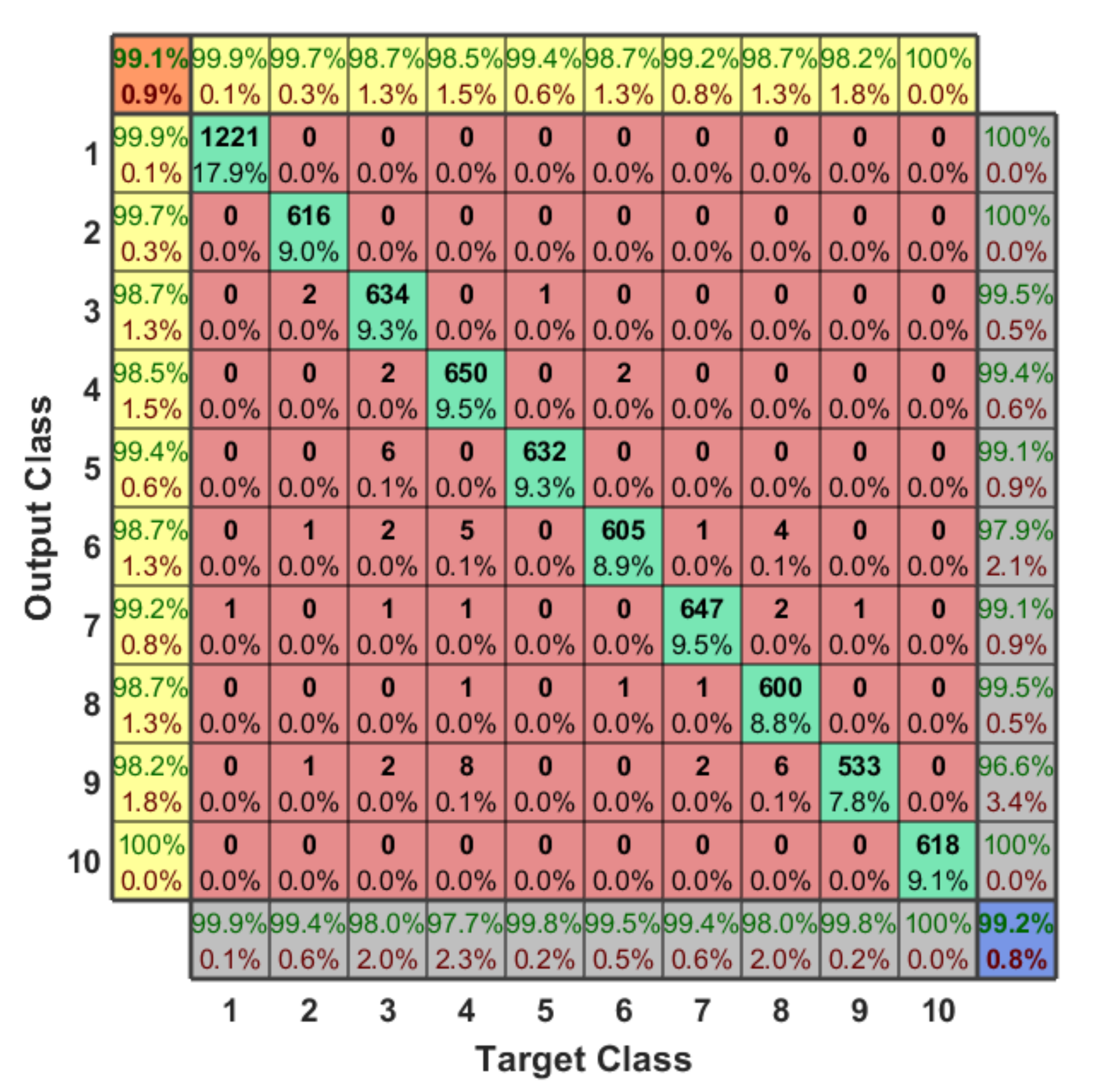
34]. In our case, and based on the RF dataset, we labeled our 10 classes using hot encoding in order to solve this 10-classes problem, and each sample has a specific label with respect to our classes from 1 to 10. Therefore, the final output of any testing sample specifies the presence of the UAV, the type of the detected UAV, and the flight mode of this UAV.
Figure 12 shows the confusion matrix of the 10-classes problem. The classification accuracy is 99.20%, average F1 score is 99.10%, recall is 99.11%, the average detection error is around 0.80%, and the testing time for any sample to be detected correctly is in range of 6.54 msec and 7.41 msec in all scenarios.
We can conclude from the confusion matrix of our learning approach that solving the detection problem in a hierarchical manner minimizes the error value. Since, we are dividing our problem into four small classification problems with respect to the testing sample, each classifier finds the target class of the sample and then forwards the testing sample to the next classifier, and so on, until specify the type and flight mode of the detected UAV. Based on our dataset for the first classifier, we notice that it is easy to determine the presence of the UAV since each RF data has different variations from the other one, where the error value here is almost zero (one sample is only detected wrong). Therefore, we have only two classes, either “No UAV” or “UAV”. In order to define the type of the UAV, we need to enter the second classifier. The output of this classifier is one class out of three classes (Bebop, AR, and Phantom 3). Since we have only one flight mode for the Phantom 3 based on our RF dataset, this considers directly as class 10. On the other hand, if the testing sample is not Phantom 3, it enters the next classifier (4-classes) in order to specify the flight mode based on the detected type (Bebop or AR) from previous classifier. For Bebop, we have 4 classes (from 2 to 5) and 4-classes for AR (from 6 to 9).
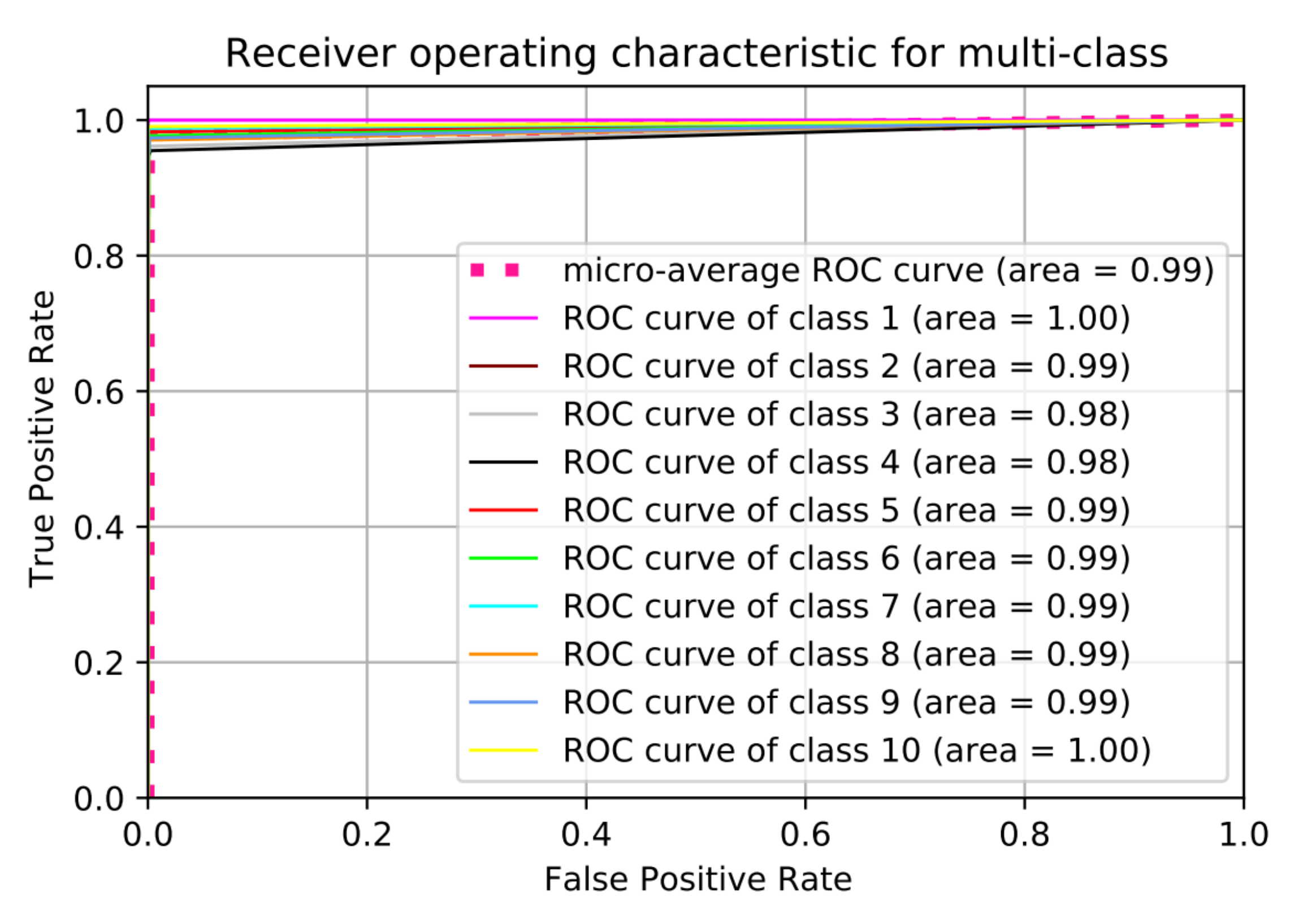
Somehow, we notice that the classification accuracy decreases when the number of classes increases. Class 2 to class 9 have same range of RF values (Bebop and AR) for different flight modes since they are produced by same company so that the detection accuracy is low compared with phantom UAV. On the other hand, the recall values remain high for the 10 classes with value around 99.11%. We plotted the Receiver Operating Characteristic (ROC) curve. It is a useful tool to predict the probability of a binary output. The
x-axis of the figure represents the False Positive Rate (FPR) and the
y-axis represents the True Positive Rate (TPR) with different probability values from 0 to 1 for the classes.
Figure 13 shows the ROC, along with the Area Under the ROC curve (AUC), of our approach with 10 classes based on the optimal hyper-parameters.


 ,
, 


