1. Introduction
It is known that concrete is a non-uniform building material made of cement, sand, water, coarse-grained materials and so on [
1]. Image-based concrete surface defect detection can realize automatic positioning [
2,
3], but internal defects are still difficult to detect. Currently, ultrasonic technology is widely used in the detection of internal defects in concrete because of its strong penetrability and high sensitivity [
4,
5]. Ultrasonic detectors applied in the actual project judge health statuses of test objects by analyzing ultrasonic information, the propagation time, amplitudes, etc. of the ultrasonic pulse velocity [
6]. This method is primarily based on physical information from ultrasonic pulses and has high accuracy when detecting homogeneous media such as metals [
7]. However, the heterogeneity of concrete causes more noise or serious waveform distortion in ultrasonic detection signals. This creates difficulty in obtaining accurate detection results within the recognition results, using recognition methods based on ultrasonic echo waveforms. Moreover, recognition of signal characteristics requires good technology and experience on the part of the inspectors, and has low detection efficiency and accuracy [
8].
More recently, there have been numerous applications of machine learning intelligence algorithms to identify ultrasonic detection signals based on signal processing methods in the time and frequency domains, combining efficient feature extraction methods. Oh [
9] used a support vector machine to identify the strength grades of concrete based on ultrasonic detection signals, but the classification accuracy was less than 90%. Saechai [
10] used a novel method based on a support vector machine to identify defective concrete ultrasonic detection signals, and its classification accuracy was higher than 93%. Furthermore, the experimental concrete blocks used in these studies did not add coarse aggregates and the artificial defect sizes were large, causing detection echo signals to have a relatively considerable difference based on practical concrete engineering. Hu [
11] used a genetic algorithm optimized back propagation neural network to identify the ultrasonic signals of concrete defects and the average recognition accuracy is 91%. Zhao [
12] used the stochastic configuration network to identify the ultrasonic detection signals of concrete defects and the accuracy is around 95%. Their experimental data were collected from concrete blocks of C30 class containing hole defects using the ultrasonic testing system [
13]. These machine learning methods do not easily devise higher recognition accuracy for complex ultrasonic detection signals of either small or medium-sized defects in concrete [
14].
Currently, deep learning algorithms are the most popular pattern recognition methods to perform specific tasks in more and more fields. Deep learning has the advantages of strong learning ability, good generalization, and convenient transplantation, but also has the disadvantages of large data demand and long training time [
15]. As computer performance increases, these will no longer be major challenges. However, in the field of ultrasonic inspection, the application of deep learning algorithms is focused on image recognition after ultrasonic imaging, acquiring complex imaging algorithms to pre-process the detection signals [
16]. The one-dimensional convolutional neural network (1DCNN) algorithms, can be directly used for signal classification. For instance, 1DCNN algorithms were applied to the fault diagnosis of bearing vibration signals [
7] and the abnormality discrimination of heart sound signals [
17], and their recognition accuracies were up to more than 99%. Simultaneously, Munir [
18] applied a CNN to the classification of ultrasonic detection signals of metal welds and proved that the method is effective for defect recognition of ultrasonic signals. Compared with homogeneous materials, the ultrasonic detection signals of concrete contain more mixed and disturbing noise signals [
19], such as reflected waves and transverse waves. In general, detection signals can be denoised before CNN performing classification and recognition computation. Fourier transform (FT), empirical mode decomposition (EMD) and wavelet package transform (WPT) [
20,
21,
22] are commonly used frequency-domain methods for ultrasonic signal processing. Comparatively, wavelet transform is one of the most widely used methods in ultrasonic detection signal processing of concrete because of its improved time-frequency analysis ability [
23,
24].
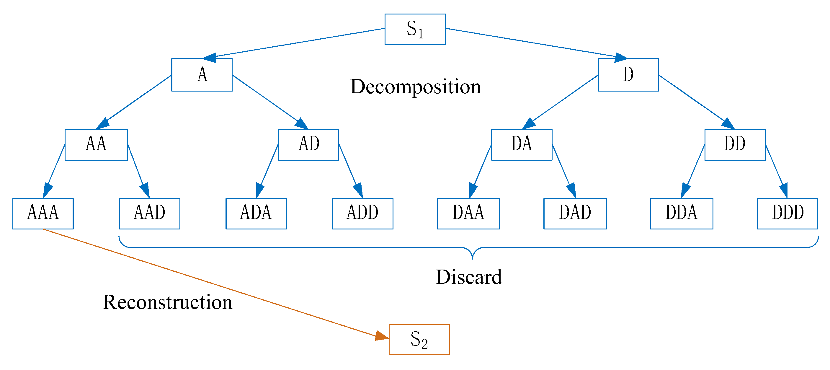
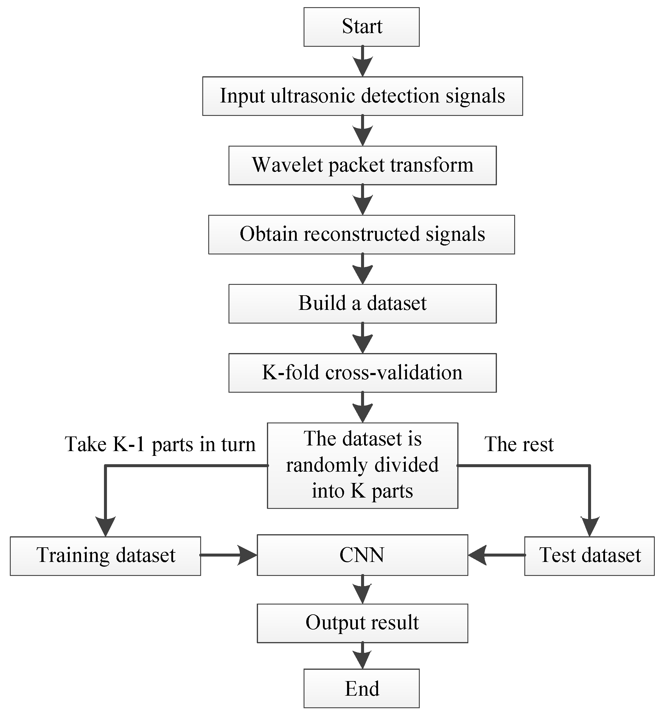
For the purpose of developing an intelligent analysis and automated recognition of concrete ultrasonic defect signals, an effective method for WPT and CNN is proposed to diagnose the ultrasonic fault signal, whereafter the received ultrasonic detection signals are processed by a specific WPT sub-algorithm, and a specifically trained CNN model is used to automatically identify the types of concrete defects. The proposed method comprises WPT sub-algorithms to reconstruct fundamental frequency signals from ultrasonic detection signals, which provides coefficients in the first node of the third layer after three-layer decomposition of the wavelet packet. A specific 1DCNN sub-algorithm of eight layers altogether performs extracting features from the processed A-Scan signals, reducing the effective features loss or inaccurate feature extraction caused by artificial feature extraction, and realizing the automatic classification of concrete defect types. In addition, we operated the stochastic configuration network method (SCN) [
24] for comparison and performance evaluation. On the other hand, the K-fold cross-validation method is applied to the classification experiment to verify the contingency of a single experiment result and reflect the performance of the model more accurately; even CNN algorithms possess the computational structure to prevent overfitting and underfitting. Through the ultrasonic detection signal classification experiment, three types of hole defects and no defect of a C30 class concrete block and a concrete block containing crack and foreign body defects are detected. Then, these detected experimental datasets are imported into the proposed method to verify their effectiveness, accuracy rate, etc. Simultaneously, the indicators are obtained to evaluate the algorithm performance. Our contribution is based on realizing the automatic classification of concrete ultrasonic detection signals and improving the diagnostic accuracy of the detection results on previous machine learning methods.
The paper is organized as follows:
Section 2 describes the algorithm involved in this paper in detail, especially the structures and steps in the algorithm;
Section 3 describes the experimental objects, data, and algorithm parameter settings;
Section 4 has our experimental results and the relevant analysis of algorithm performance; finally, the correlational experimental results and conclusion are given in
Section 5 and
Section 6.
3. Experimental Environment and Algorithm Parameter Settings
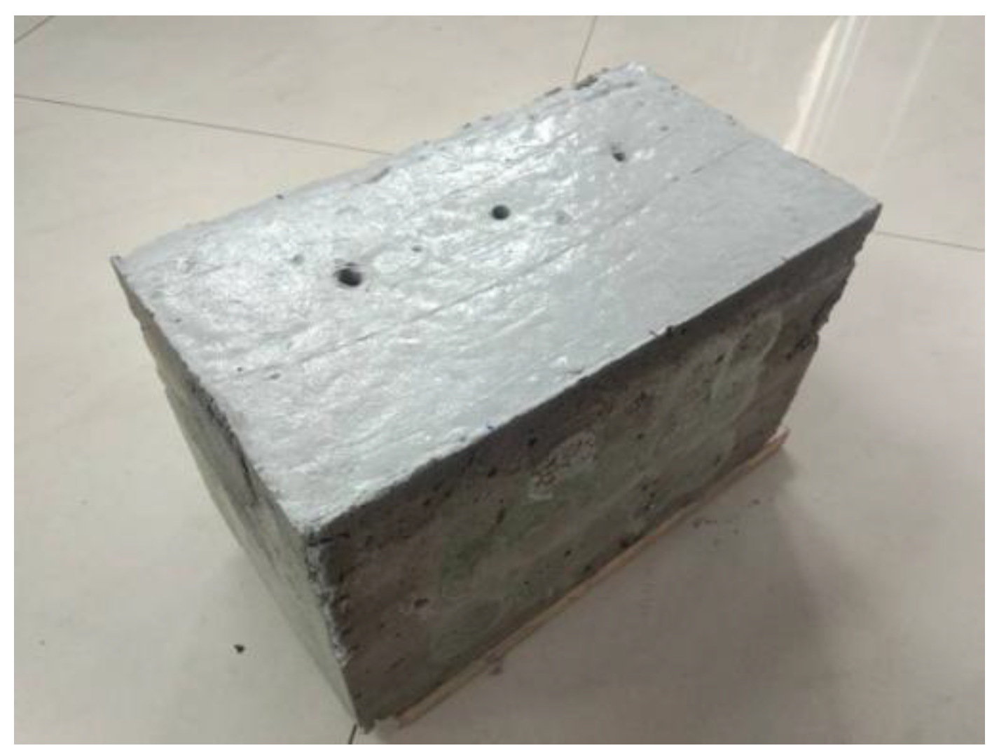
The test data are from the ultrasonic testing experiment, 50 kHz low-frequency ultrasonic probes are used, and the detection method is the ultrasonic transmission method. We applied couplant on the surface of detection positions of the concrete to remove the air between probes and the concrete blocks, so that the ultrasonic probe can penetrate the concrete effectively. The experiment objects used for ultrasonic testing in this case study are two C30 class concrete blocks shown in
Figure 5 and
Figure 6. All concrete test blocks are made by mixing ordinary Portland cement type I, water, sand, and gravel at the ratios of 461, 175, 512, and 1252 kg/m
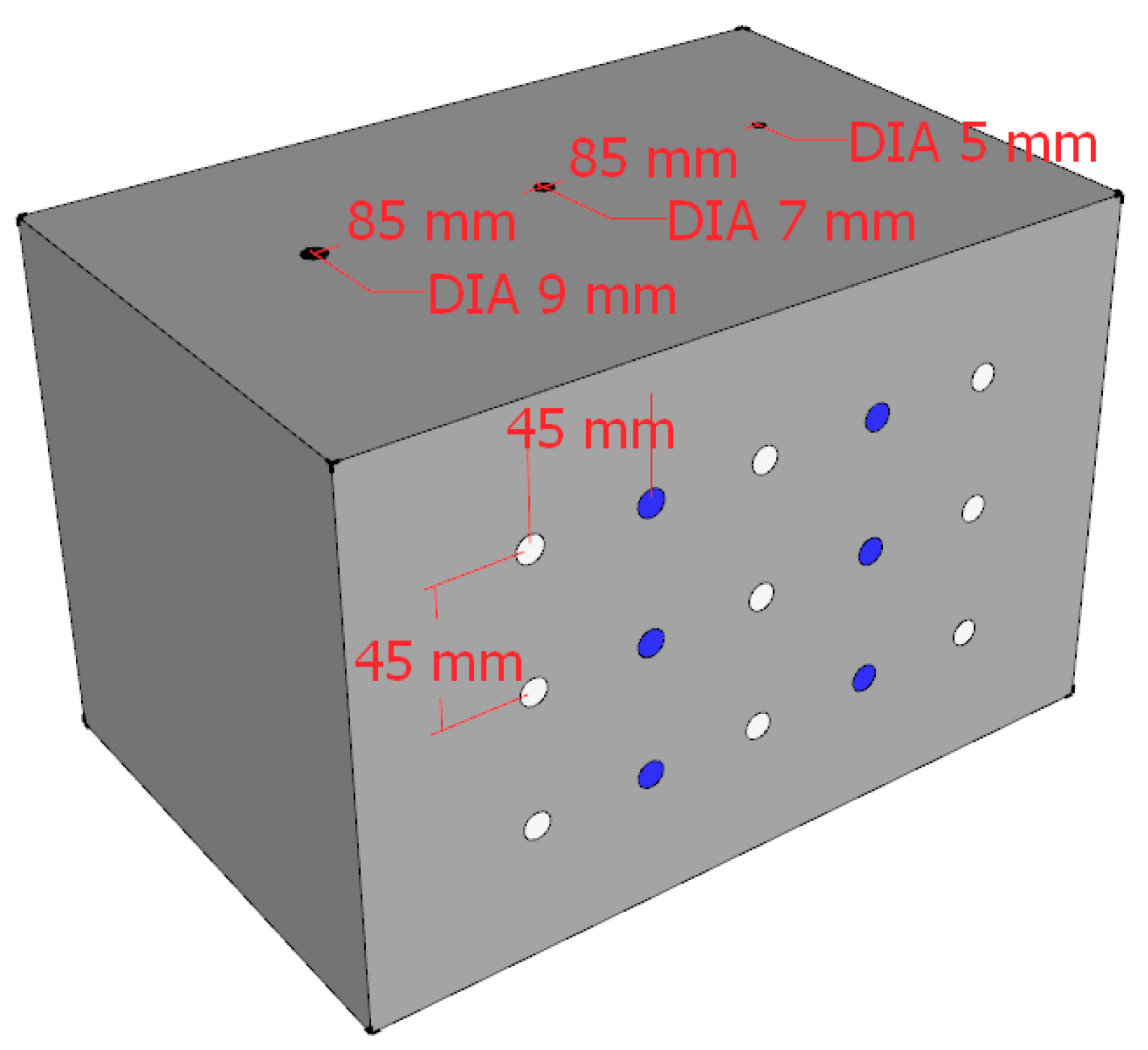
3, respectively. The sizes of the two concrete samples are the same, 300 × 200 × 200 mm. One of the concrete blocks contains three sizes of hole defects with diameters of 5 mm, 7 mm, and 9 mm. The distance between two penetrating holes is 85 mm, which is shown in
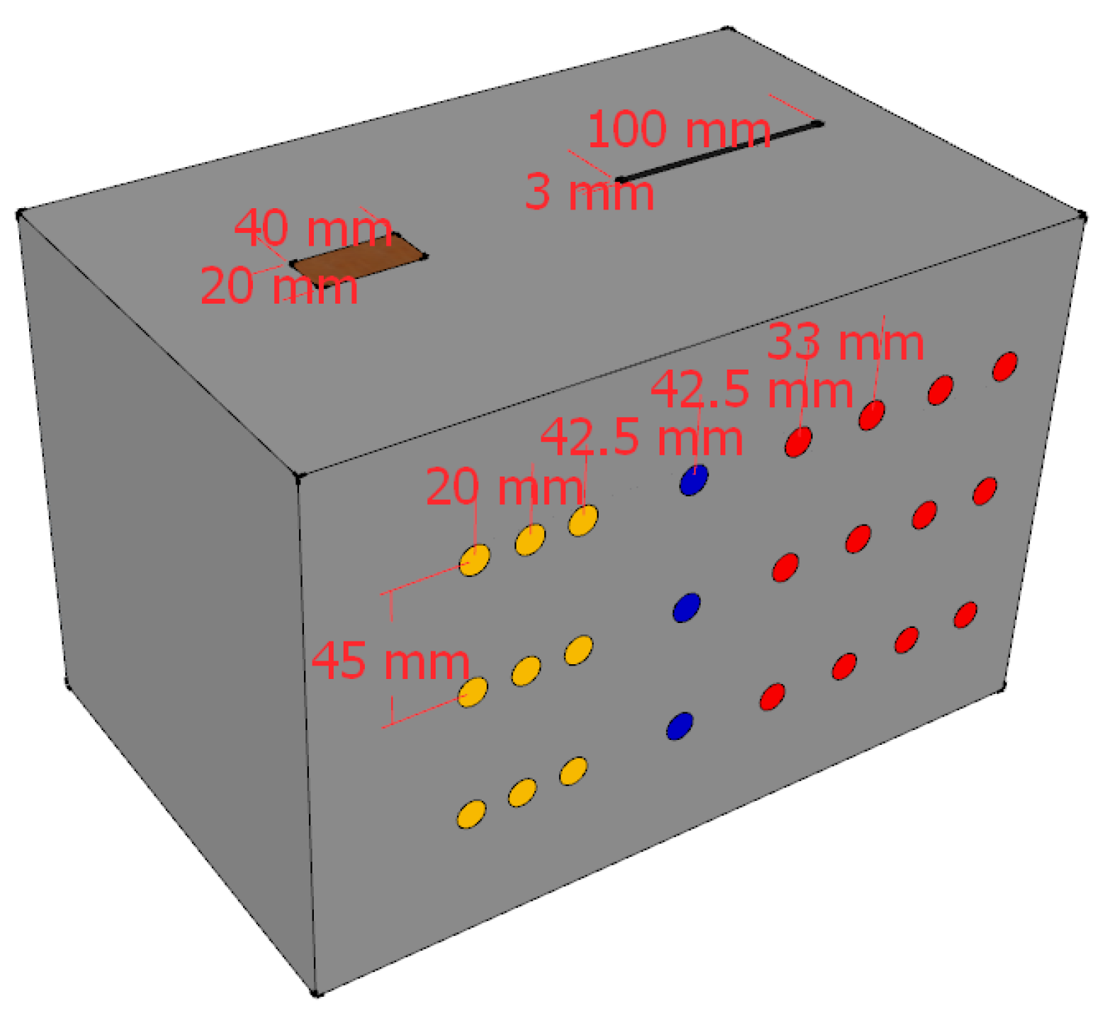
Figure 5. Another concrete block contains crack and foreign body defects. The size of the crack is 100 × 3 mm. The size of the foreign matter of wood is 40 × 20 mm. The distance between the two defects is also 85 mm. The material object is shown in
Figure 6. The defects penetrate the concrete blocks so that we can observe the actual locations of the defects.
Figure 7 and
Figure 8 show the schematic diagrams of the detection positions. In the figures, the blue points, white points, red points, and yellow points locate the detection positions of no defect, hole, crack, and foreign matter, respectively. The center distances between the detection points arranged on the surface of the concrete block are shown in
Figure 7 and
Figure 8.
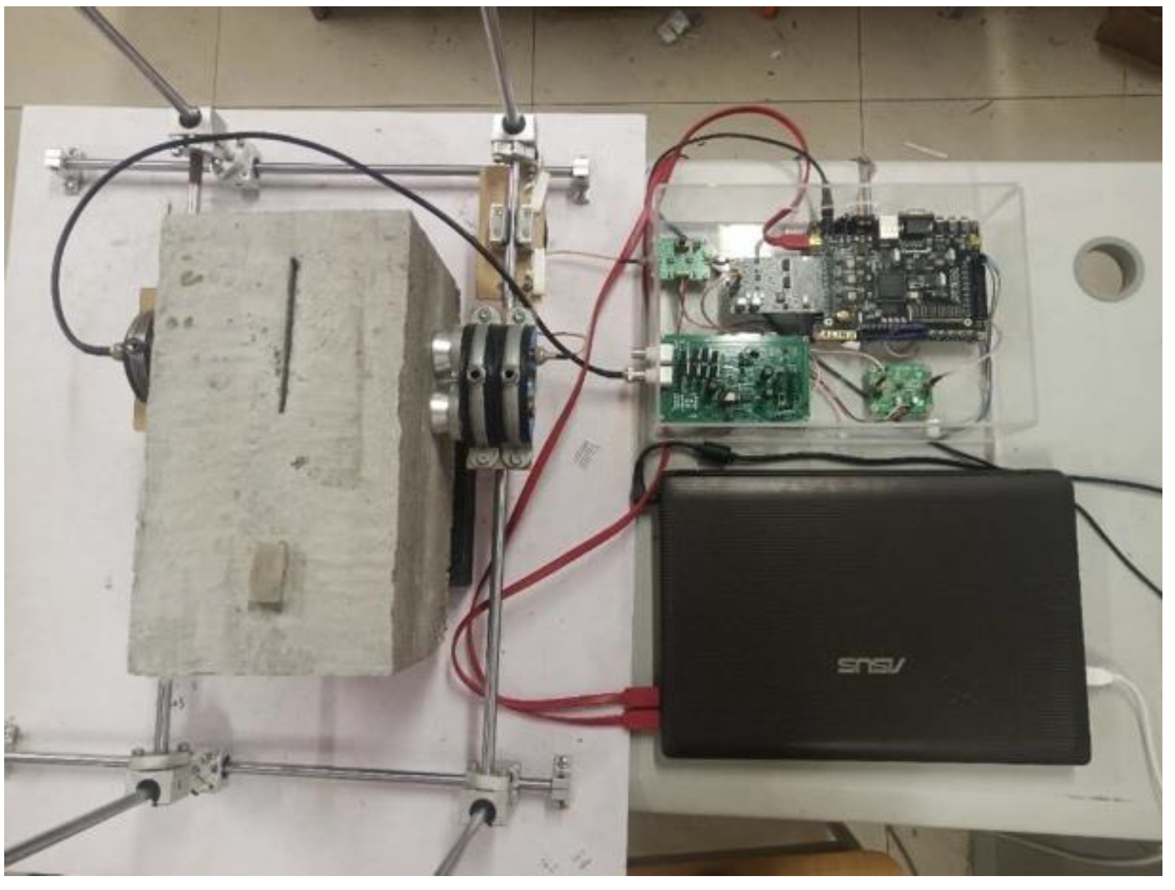
Figure 9 shows the ultrasonic detection hardware system used in our experiments. The working performance of the hardware system that we evaluated in the published paper is reliable. The receiving end of the detection system is equipped with a spare probe. In the experiment, the transmitter produces ±100 V square wave pulse signal is used to excite the ultrasonic probe, and the signal sampling frequency at the receiver is 1 MHZ. The size and category of datasets are shown in
Table 1. Each sequence contains three cycles of ultrasonic detection signals, with a total of 12,000 sampling points.
The proposed algorithm proposed in this article runs on a computer with Windows 10 64-bit operating system. The CPU specification is 6-core 2.08 GHz Inter Core i5-8400, and the memory specification is 32 GB 2400 MHz DDR4. The software used includes MATLAB 2014b and Python 3.7. The main parameters setting of the WPT-CNN algorithm are listed as follows.
The main parameters of the WPT sub-algorithm are: db15 is used as the wavelet basis function to perform 3-layer decomposition; Shannon entropy is calculated and used as the optimal wavelet basis. The fundamental frequency of ultrasound in this paper is 50 kHz. According to the frequency range of each node after decomposition, the first node of the third layer is extracted to obtain the reconstructed signal.
The parameters of K-fold cross-validation method are set as follows: K = 5, N = 5400. K represents the number of divided data and the number of classification experiments, and N represents the total amount of data. Under K-fold cross-validation, the data are randomly divided into five parts, four parts with a total of 4320 sequences are the training dataset, and the remaining part with a total of 1080 sequences are the test dataset. To adjust the hyperparameters of the model and to conduct a preliminary evaluation of the model’s ability, we select 620 sequences from the training set as the validation set. For the four-classifying model, data from three sizes of hole defects are trained and identified as the same kind. For the six-classifying model, data from three sizes of hole defects are trained and identified as three kinds of defects. For the five-classifying model, data from 5 mm hole defects are not used for the training dataset and validation set but for the test dataset, and they are expected to be identified as two kinds of hole defects.
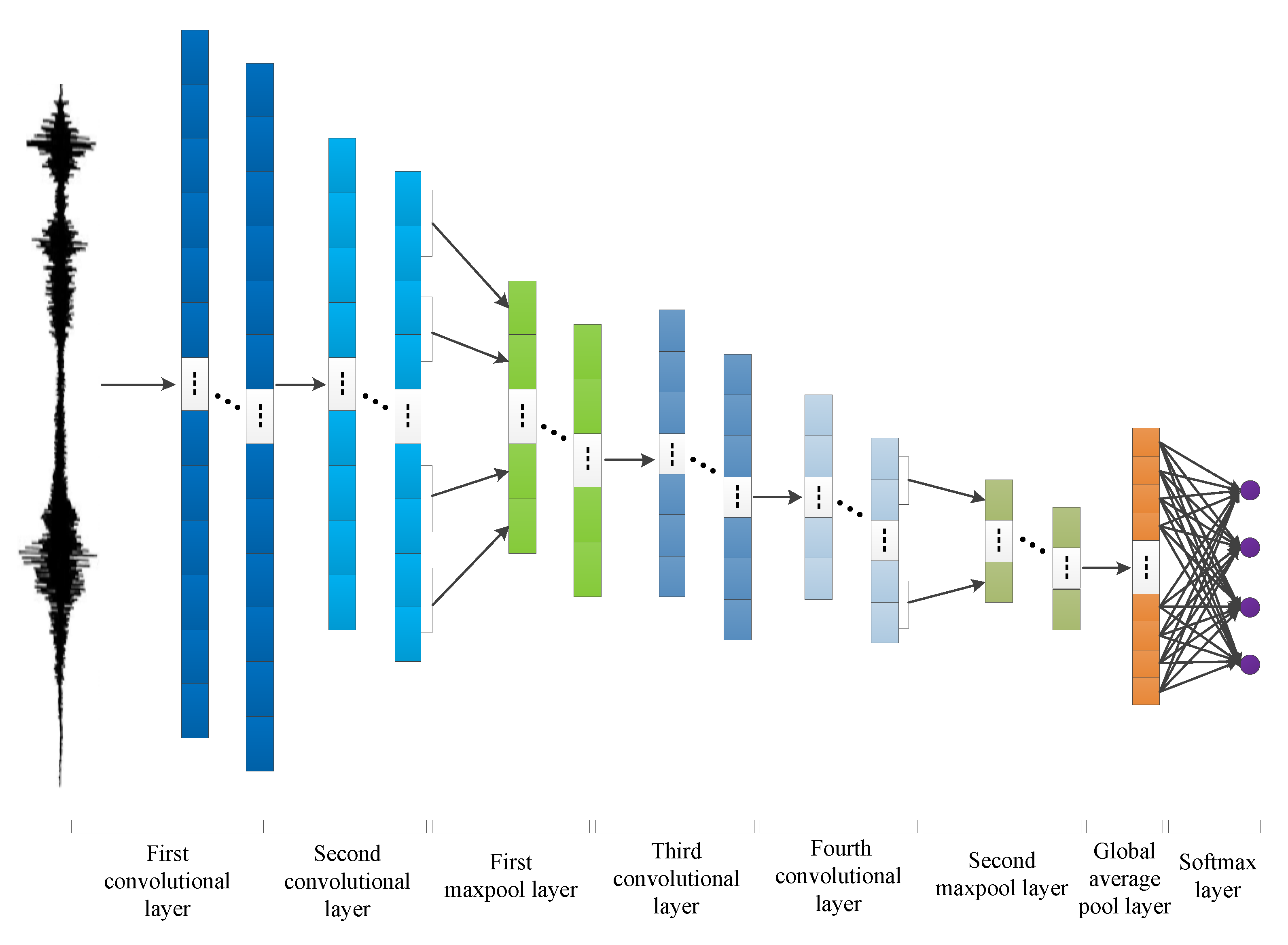
The network structure of CNN sub-algorithm is shown in
Figure 2 in
Section 2. The parameters of the CNN sub-algorithm are as follows. We set the number of training times to 200 and the batch size to 100. The first layer of convolutional layer has 64 convolution kernels, the size is 8, the step size is 4, and the filling method is the same. The parameters of second convolutional layer are the same as the first layer. The first layer of pooling layer adopts the maximum pooling method, the size of the convolution kernel is 2, and the step size is 1. The third convolutional layer has 128 convolution kernels, the size of the convolution kernel is 4, and the step size is 2, and the filling method is the same. The fourth convolutional layer has the same parameters as the third, and the second pooling layer uses the maximum pooling method. The above layers all use the rectified linear unit (ReLU) as the activation function. The third layer of the pooling layer adopts the global average pooling method, and the node retention probability of random inactivation (dropout) is set to 0.3; the last softmax layer has four nodes, and the softmax function is used. When training the model, we use the cross entropy as the loss function, we use the Adam optimizer, and set the learning rate to 0.001.
The stochastic configuration network parameters are set as follows [
12]. The maximum number of hidden layer nodes
L is 200 (one epoch is performed when
L is accumulated for one cycle), the training error is 0.01, and the activation function is the Log-sigmoid transfer function (logsig). The maximum number of random configuration is 100, the random weight range is {0.5, 1, 5, 10, 30, 50, 100}, the inequality constraint coefficient is {0.9, 0.99, 0.999, 0.9999, 0.99999, 0.999999}, set step length to 1 as the number of hidden layer nodes is accumulated.
4. Experimental Results and Analysis
4.1. Reconstructed Signals by the WPT Sub-Algorithm
After the three-layer decomposition of the wavelet packet is processed, the energy ratio of the signal component in each node is calculated, which is the sum of the squares of the wavelet packet coefficients, as shown in
Figure 10. The greater the energy, the higher the value of the wavelet packet coefficients [
35]. Based on the characteristic of energy distribution, the fundamental frequency node of the signal is self-explanatory. Naturally, the first node coefficients of the third layer are used to reconstruct them into complete signals due to this result.
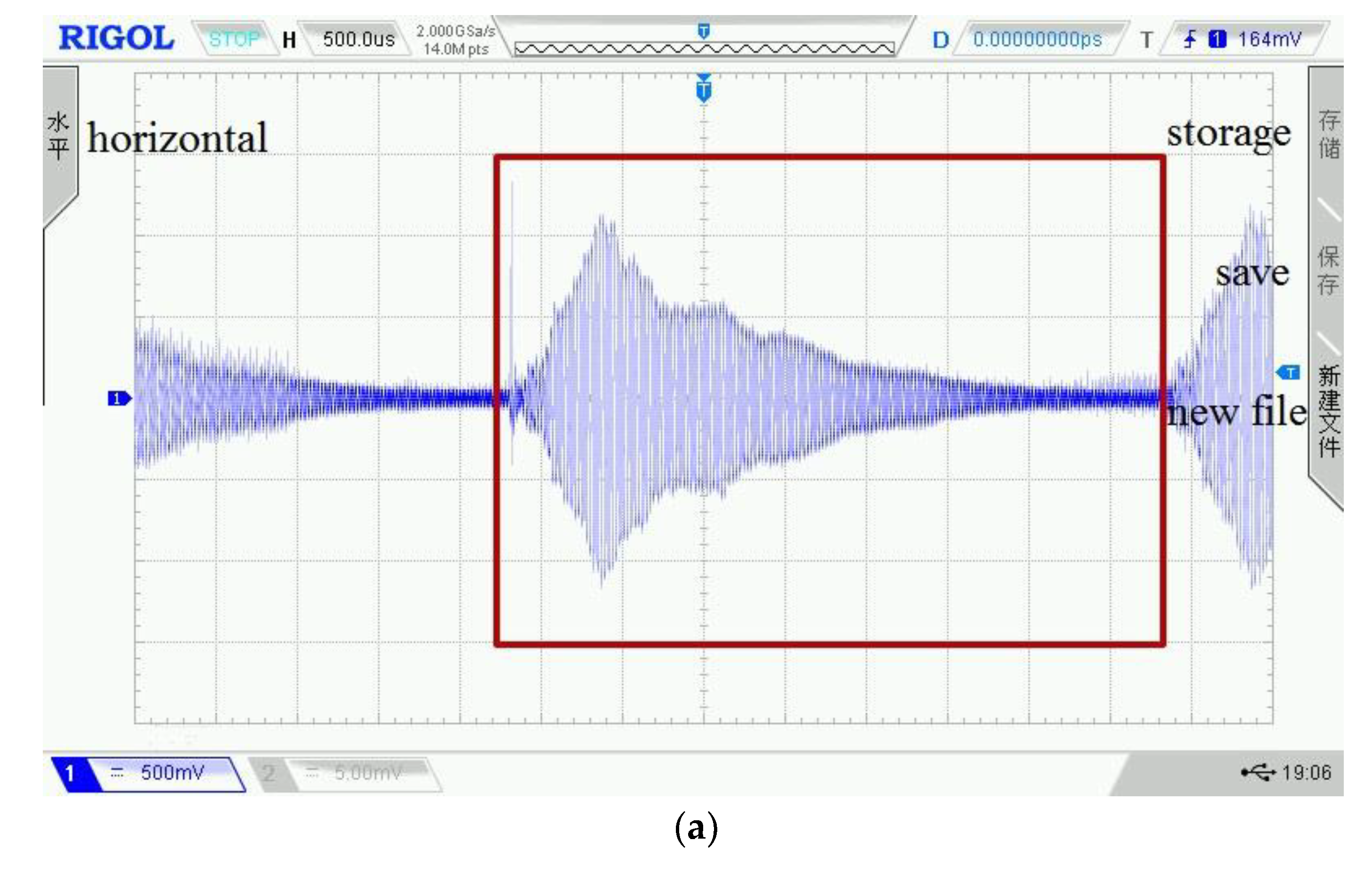
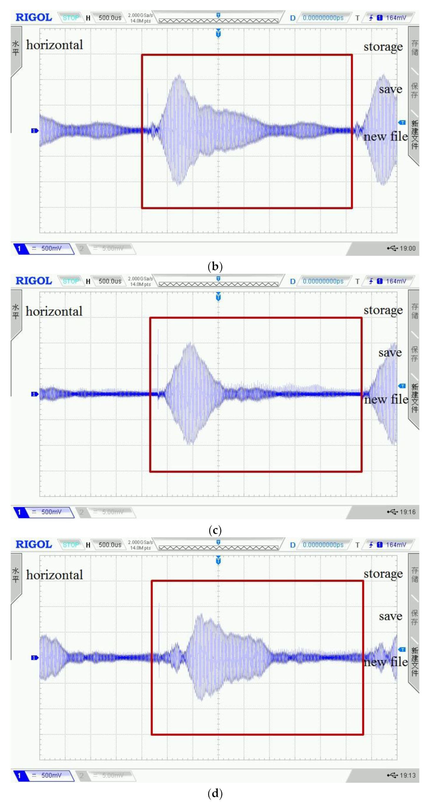
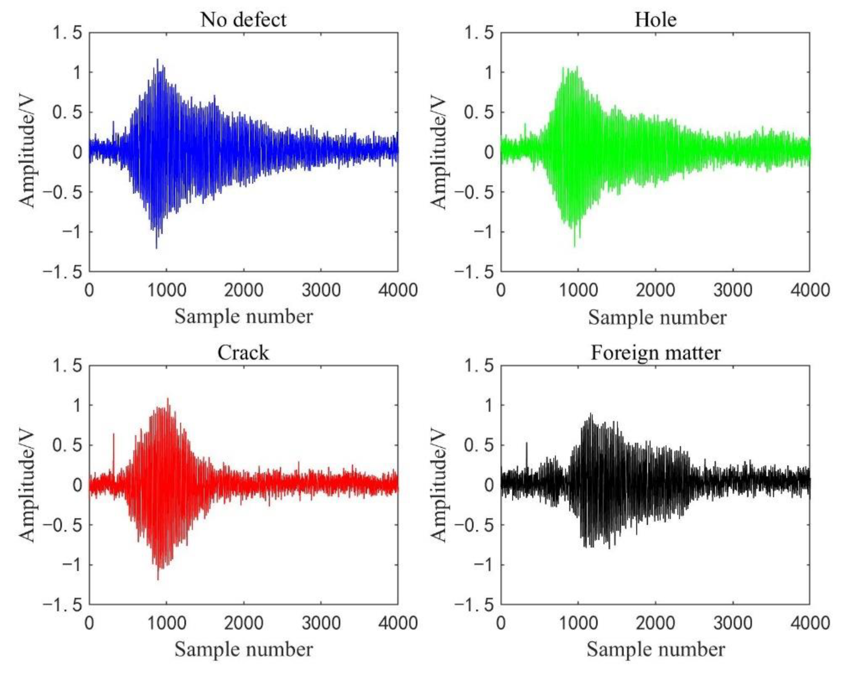
Figure 11 shows the waveforms of four kinds of detection signals displayed on the oscilloscope, where the wave in the red box is a complete cycle signal data sequence. In addition, four displayed waveforms are randomly selected from the detection dataset of four kinds of concrete conditions. To display the waveform curves before and after processed by the WPT sub-algorithm, we draw the last cycle of the selected signals in
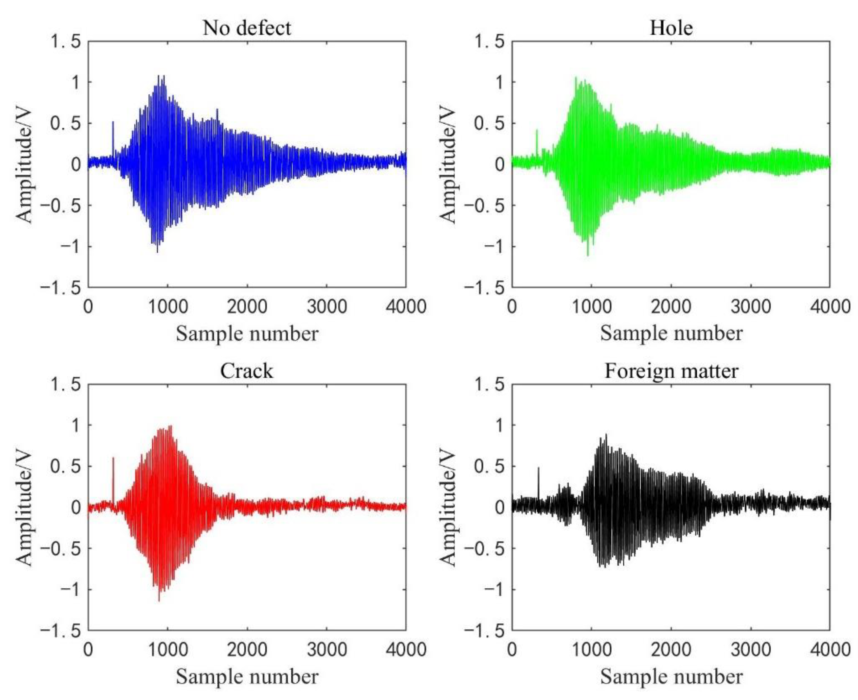
Figure 12 and their reconstructed waveforms in
Figure 13. It shows that the reconstructed detection signal waveforms are smoother by comparison with
Figure 12 and
Figure 13. High-frequency noise is almost removed from the reconstructed waveform, which perhaps reduces the impact of high-frequency noise on the accuracy of the classification model.
4.2. Four-Classifying Model
The five-fold cross-validation method randomly divides the sample set into a training dataset (including validation dataset) and test dataset [
36]. Each subset is taken out of the total sample set by uniform random sampling to ensure that the proportion of sub-samples is consistent with the overall sample. As is well known, the training dataset is used to optimize model parameters, the verification set is used to adjust hyperparameters, and the test dataset is used to verify the generalization ability of the model [
37,
38]. When the CNN sub-algorithm is applied to concrete ultrasonic detection signals to build the four-classifying model, the stochastic configuration network algorithm is introduced as a comparison model simultaneously. To analyze the performance of the CNN model, the error and accuracy change curves were illustrated during the training process in an experiment with the highest test accuracy.
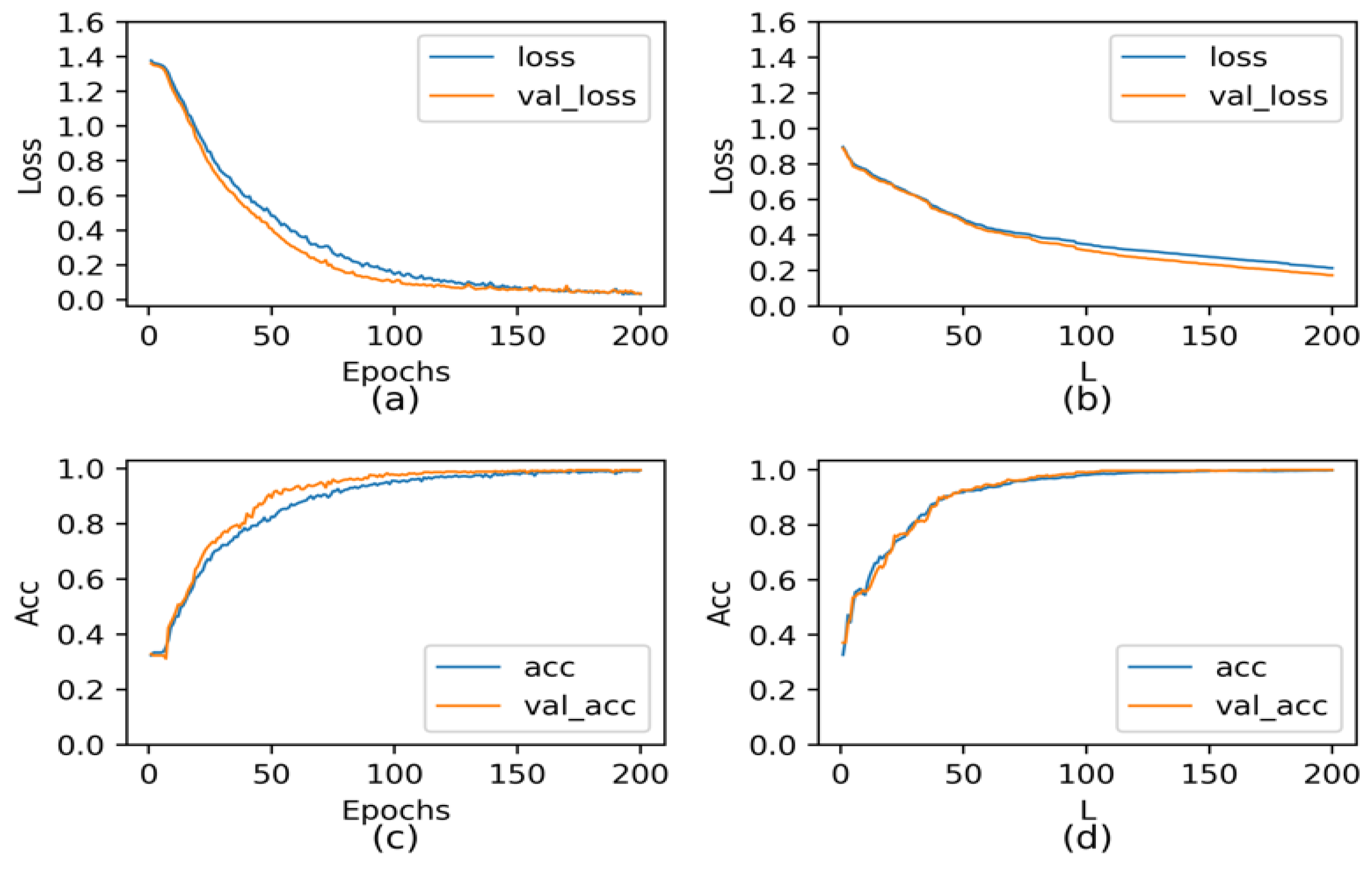
As shown in
Figure 14a,b, the error curves of two models on the training dataset and validation dataset are plotted, respectively, where the blue curve is the error change curve of the training dataset and the orange curve is the error change curve of the validation dataset.
Figure 14c,d shows the classification accuracy change curves of CNN and SCN models on the training set and validation set. It can be seen from
Figure 14 that the rate of convergence of CNN model is less than that of SCN model, and the final training error is less than that of SCN model. The classification accuracies of CNN on the training dataset and validation dataset during the training process are both higher and close to 100%. With the increase of epoch, the classification accuracy of SCN model on the training set tends to be stable.
The highest, lowest, and average accuracy rates among the five results of the two models are listed in
Table 2, owing to five-fold cross-validation. The recognition accuracy values of five CNN models all exceeded 99%. The difference between the highest accuracy and the lowest accuracy is only 0.28%, which is very small and reflects the imitative effect. The comparison with the recognition accuracy of SCN shows they are lower than the CNN model, and their difference is around 1%. Then, CNN model has higher classification accuracy for concrete ultrasonic detection signals and is more stable, but it needs a lot more time for training and testing. In this paper, the processor of computing environment is CPU. High-performance computing equipment such as GPU, has been used for intelligent computing, and the running time of CNN model will be greatly reduced. Similarly, if the time cost is acceptable, then the application of CNN sub-algorithm to ultrasonic testing equipment will not be so difficult.
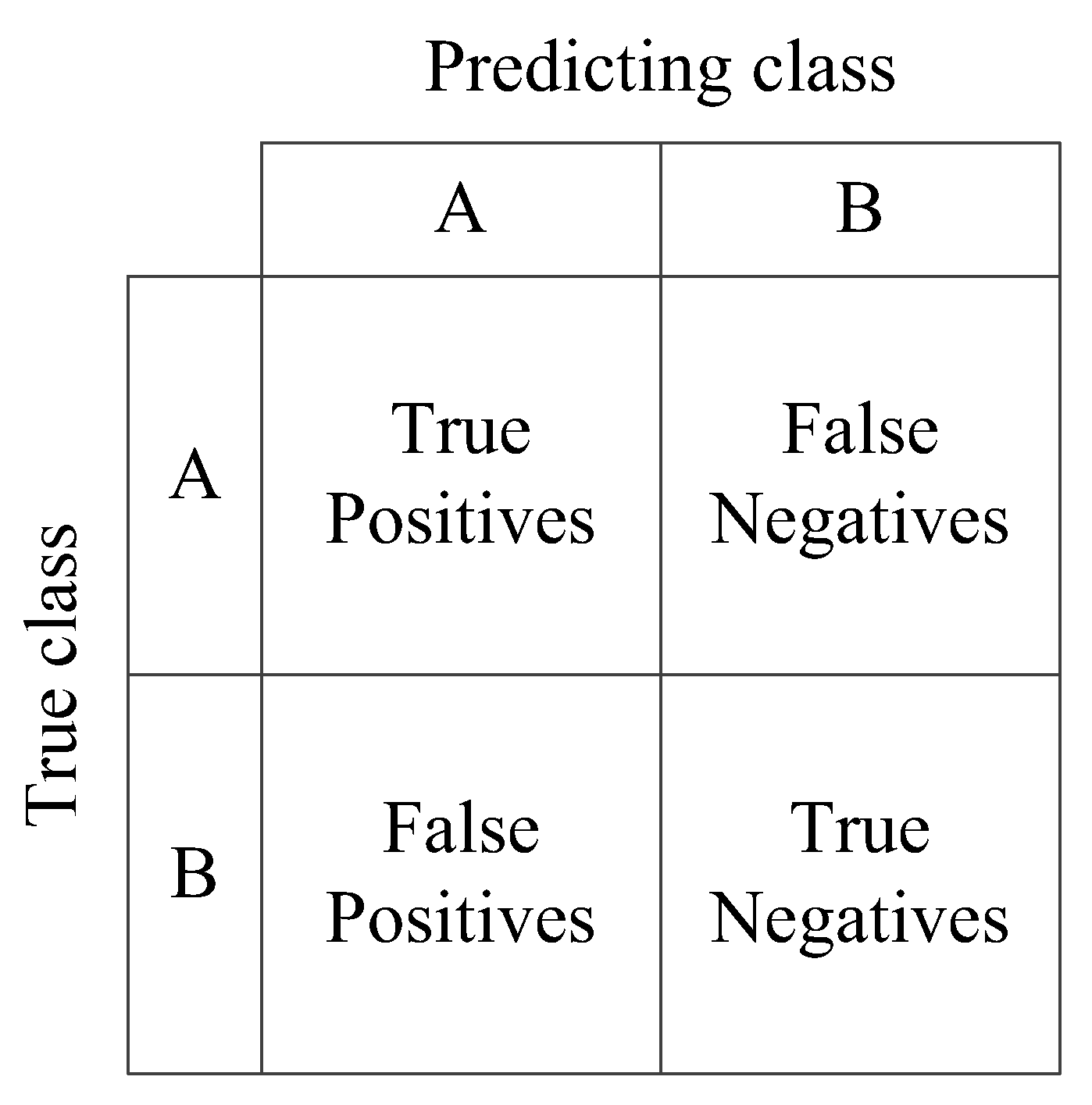
Table 3 shows the accuracy, recall, and F-score of two models are calculated for evaluating performance on different detection signal types. The four indices of CNN model are higher than those of SCN model, especially for the recognition accuracy of detection signals of the foreign matter defect. CNN models have the highest overall classification accuracy on four types of detection signals.
The recognition accuracy of CNN model of the concrete ultrasonic detection signal is higher than 99%, but still cannot reach 100%. Furthermore, it is true that when detecting similar defects in different positions of concrete blocks, the obtained detection signals have uncertain differences. For example, the built dataset contains 200 data samples detected from four edges of crack and foreign matter defects. These signals are quite different from signals detected from the middle positions. Spontaneously, this leads the recognition accuracy of the classification model not to reach 100%. On the other hand, there are some random links in the operation of neural networks, such as the initial weights and thresholds of CNN and SCN, the randomness of regularization, etc. [
39,
40], which will cause the model classification accuracy fluctuate every time. From another perspective, the classification results processed by five-fold cross-validation, fluctuate in a small range, and indicate that the CNN model has strong stability and generalization ability.
4.3. Six-Classifying Model
The six-classifying experiment for CNN model is analogous to the above four-classifying experiment, but three sizes of hole defects are treated as three different defects. In this classification experiment, the five-fold cross-validation partition datasets for training and testing are still used. Finally, five test results from the CNN and SCN models are obtained. The highest, lowest, and average accuracy rates among the five results of the two models are listed in
Table 4, and the precision, recall, and F-score of the two models are listed in
Table 5.
The running times of ten models are essentially unchanged because the data size has not increased. The lowest accuracies of the two models both reach more than 95%. In addition, CNN classification performance is better than in the SCN models according to four evidence indices. Compared with the four-classifying experiment, the recognition accuracies of this experiment decreased slightly. One reason is that the data size of three types of hole defect is about half lower than those of other three types of defects. In this experiment, the hole data are divided into three categories, so the complication of classification features of hole defeats is increased compared to that of the four-classifying CNN models and SCN models. Subjectively, it shows that the small difference of defect sizes makes their classification calculated by CNN models or SCN models more difficult. The results show that the proposed WPT-CNN method has a certain effectiveness in more complex detection and has higher practical engineering significance.
Some evaluation index values of the three sizes of hole defect decrease significantly compared with the values in
Table 3; in particular, the recall of 5 mm hole defect is the worst. The reason for this is that CNN models confuse a 5 mm hole defect with the other five types of defects, and the 7 mm hole defect, 9 mm hole defect, and crack defect account for the largest number according to their precision and F-score values. Therefore, defect identification of different sizes will be the subject of one of our future studies.
4.4. Five-Classifying Model
Being curious about the recognition effect of the unknown detection data on WPT-CNN models, we proceed the five-classifying experiment. According to the five-classifying experiment, some interesting results and analysis are shown in this section.
The five-classifying experiment for CNN and SCN models is quite different from the six-classification experiment in that the dataset used for building models does not consist of 5 mm hole defect data. First, five types of data are used to build training, validation, and test dataset, where their data sizes are 3360, 480, and 960, respectively. The same data are from 1500 sequences from non-defective detection points, 1200 sequences from hole defect detection points (600 from 7 mm and 9 mm hole defects equally), 1100 sequences of crack defect detection data, and 1000 sequences of foreign matter defect detection data. Then, to train and test the five-classifying CNN and SCN models in the same way of four-classifying experiment. Then, all the 5 mm hole defect data are used as additional test dataset to obtain their identification results. Here, it is regarded as a positive result that the 5 mm hole defect data are recognized as a type of 7 mm or 9 mm hole defect data.
The recognition accuracies and evaluation indices of the five-classification experiment are listed in
Table 6 and
Table 7, respectively. Experimental results of testing 5 mm hole defect data are presented in
Table 8, where the highest and lowest percentages are the highest and lowest positive percentages of 5 mm hole defect data that are correctly identified as two types of hole defects of five models. The average percent is the average value of each value across five experiments.
The data size of the dataset in this experiment is less than those of the above two experiments, so it takes less runtime to build the models. Compared with the recognition accuracies of six-classifying CNN and SCN models in
Table 3, those in
Table 6 are improved by about 1% on average. Then, the complexity of recognition of 5 mm hole defect data is evident. According to
Table 6, it is obvious that CNN models have a higher recognition accuracy than SCN models, especially on foreign matter data. A reason is that part of the foreign matter dataset is collected from the foreign matter edges, which contain more uncertain noise and the time uncertainty of the waveform due to heterogeneous concrete structures. It is also a major challenge in the ultrasonic detection task.
The experiment results in six tables demonstrate the validity of WPT-CNN models and SCN models for labeled detection data types. However, it is normal that data are of unknown types, obtained in actual engineering detection tasks, such as defects of unknown size. The used models are established by the above five types of data to classify the 5 mm hole defect data. Then, the positive percentage of 5 mm hole defect is the sum of two positive percentages.
It has been shown that 5 mm hole defect data are more difficult to identify from the above six-classifying and four-classifying experiments. Similarly, the highest percentages for CNN model and SCN model to identify them as hole defects are only 41% and 36.83%, and their lowest percentages are 27.17% and 24.50%. Furthermore, both 5 mm hole defect and crack defect are small cavity defects, and perhaps have some common features owing to the time uncertainty of the waveform or noise. This is an important factor for CNN models classifying 5 mm hole defect data as crack defect data at approximately 40%. Nevertheless, the CNN models identify them as the other three types of defects more than 70% of the time, which proves that the WPT-CNN algorithm has a certain effectivity to identify defect signals of unknown types. It is worthwhile to deeply study the intelligent recognition of unknown defects data.
6. Conclusions and Future Works
The proposed method to automatically classify and recognize concrete ultrasonic detection signals comprises the wavelet packet transform to decompose the original detection signal into three layers and obtain the wavelet packet coefficient of the first node in the third layer to reconstruct signals, and a one-dimensional convolutional neural network to classify and recognize the reconstructed signal data. Four identification experiments on 5400 detection data samples and a four-classifying experiment were primarily carried out, which constitutes four datasets with no defects, holes (three diameter holes), cracks, and foreign matter. Through experiments on the datasets constructed with four processing methods, WPT-CNN has the highest recognition accuracy and best generalization ability estimated by the evaluation indices, and comparison results of the stochastic configuration network. The precision and recall of the four types of signals exceed 99%, and the F-score is more than 0.99. The WPT-CNN method can effectively identify the defect signal and deploying it in the ultrasonic testing instrument can solve the current shortcomings. On the other hand, the experiment results of six- and five-classifying models, and related research on raw data and feature extraction recognition revealed the cause-and-effect factors affecting recognition performance.
Nevertheless, there are still four major challenges in applying the algorithm in this paper to ultrasonic testing instruments: data size, data nature, modeling challenges, and uncertainty [
15]. Obtaining a larger amount of data based on a variety of reliable ultrasonic detectors will be a necessary basis for algorithm application research. In the follow-up research, we will continue to optimize the algorithm model and study the application of other deep learning models, which is also an important task. The proposed method was proven to be effective for the ultrasonic detection signal recognition of C30 class concrete, and the research objects should be extended to more classes of concrete. Debonding between rebars and concrete, a more complex defect, is also an important research topic for the future [
41]. In addition, the application of the proposed method to actual detection instruments is the ultimate goal of the future.


