
Reliability-Based Large-Vocabulary Audio-Visual Speech Recognition


Abstract
:1. Introduction
2. Fusion Models Furthermore, Baselines
2.1. Hybrid Baselines
2.1.1. Early Integration
2.1.2. Dynamic Stream Weighting
2.1.3. Oracle Weighting
2.2. End-to-End Baselines
3. System Overview
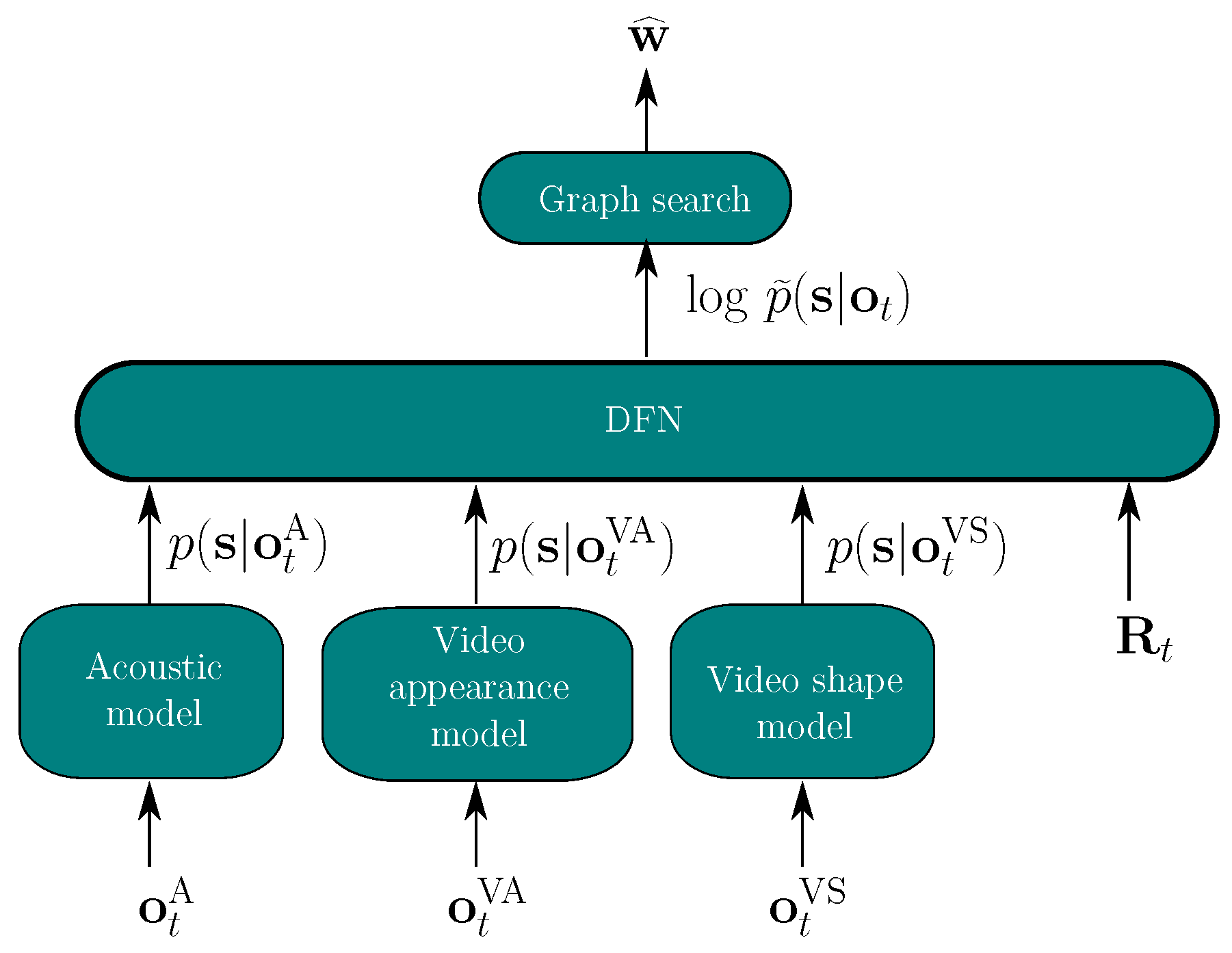
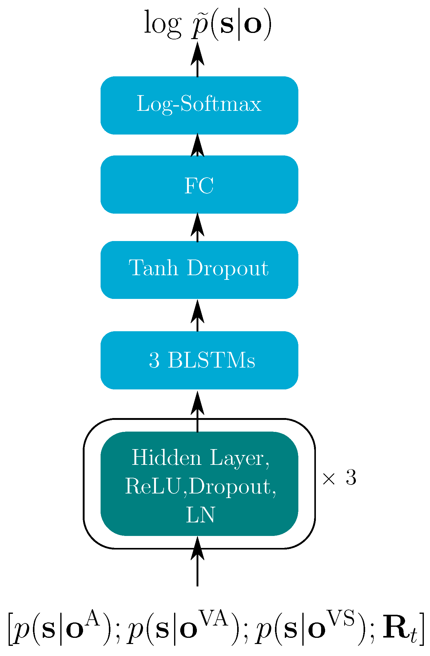
3.1. Hybrid System
3.2. E2E System
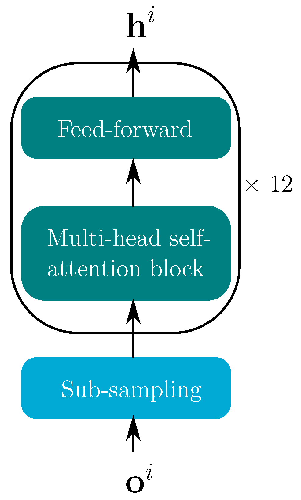
3.2.1. Encoder Architecture
3.2.2. Decoder Architecture
4. Reliability Measures
4.1. Reliabilities for the Hybrid Model
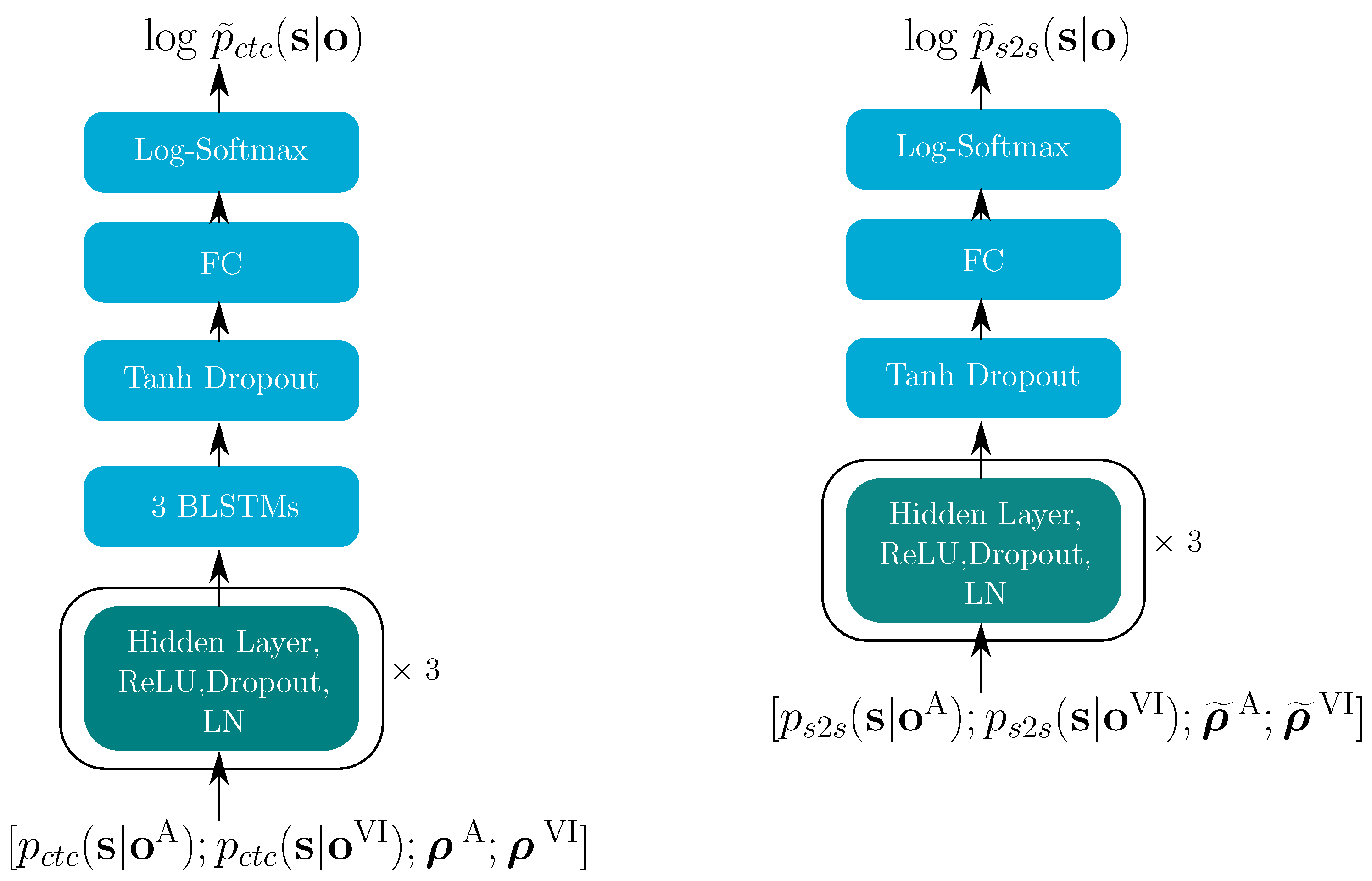
4.2. Reliabilities for the E2E Model
5. Experimental Setup
5.1. Dataset
5.2. Features
5.3. Hybrid Model Implementation Details
E2E Model Implementation Details
6. Results
6.1. Hybrid Model
6.2. E2E Model
7. Conclusions
Author Contributions
Funding
Institutional Review Board Statement
Informed Consent Statement
Data Availability Statement
Conflicts of Interest
References
- Crosse, M.J.; DiLiberto, G.M.; Lalor, E.C. Eye can hear clearly now: Inverse effectiveness in natural audiovisual speech processing relies on long-term crossmodal temporal integration. J. Neurosci. 2016, 36, 9888–9895. [Google Scholar] [CrossRef] [PubMed] [Green Version]
- McGurk, H.; MacDonald, J. Hearing lips and seeing voices. Nature 1976, 264, 746–748. [Google Scholar] [CrossRef] [PubMed]
- Potamianos, G.; Neti, C.; Luettin, J.; Matthews, I. Audio-Visual Automatic Speech Recognition: An Overview. Issues in Visual and Audio-Visual Speech Processing; MIT Press: Cambridge, MA, USA, 2004; Volume 22, p. 23. [Google Scholar]
- Wand, M.; Schmidhuber, J. Improving speaker-independent lipreading with domain-adversarial training. arXiv 2017, arXiv:1708.01565. [Google Scholar]
- Meutzner, H.; Ma, N.; Nickel, R.; Schymura, C.; Kolossa, D. Improving audio-visual speech recognition using deep neural networks with dynamic stream reliability estimates. In Proceedings of the 2017 IEEE International Conference on Acoustics, Speech and Signal Processing (ICASSP), New Orleans, LA, USA, 5–9 March 2017; pp. 5320–5324. [Google Scholar]
- Gurban, M.; Thiran, J.P.; Drugman, T.; Dutoit, T. Dynamic modality weighting for multi-stream hmms inaudio-visual speech recognition. In Proceedings of the Tenth International Conference on Multimodal Interfaces, Chania, Crete, Greece, 20–22 October 2008; pp. 237–240. [Google Scholar]
- Kolossa, D.; Chong, J.; Zeiler, S.; Keutzer, K. Efficient manycore chmm speech recognition for audiovisual and multistream data. In Proceedings of the Eleventh Annual Conference of the International Speech Communication Association, Makuhari, Chiba, Japan, 26–30 September 2010. [Google Scholar]
- Thangthai, K.; Harvey, R.W. Building large-vocabulary speaker-independent lipreading systems. In Proceedings of the 19th Annual Conference of the International Speech Communication Association, Hyderabad, India, 2–6 September 2018; pp. 2648–2652. [Google Scholar]
- Afouras, T.; Chung, J.S.; Senior, A.; Vinyals, O.; Zisserman, A. Deep audio-visual speech recognition. IEEE Trans. Pattern Anal. Mach. Intell. 2018, 1. [Google Scholar] [CrossRef] [Green Version]
- Stewart, D.; Seymour, R.; Pass, A.; Ming, J. Robust audio-visual speech recognition under noisy audio-video conditions. IEEE Trans. Cybern. 2013, 44, 175–184. [Google Scholar] [CrossRef] [PubMed] [Green Version]
- Abdelaziz, A.H.; Zeiler, S.; Kolossa, D. Learning dynamic stream weights for coupled-hmm-based audio-visual speech recognition. IEEE/ACM Trans. Audio Speech Lang. Process. 2015, 23, 863–876. [Google Scholar] [CrossRef]
- Potamianos, G.; Neti, C.; Gravier, G.; Garg, A.; Senior, A.W. Recent advances in the automatic recognition of audiovisual speech. Proc. IEEE 2003, 91, 1306–1326. [Google Scholar] [CrossRef]
- Luettin, J.; Potamianos, G.; Neti, C. Asynchronous stream modeling for large vocabulary audio-visual speech recognition. In Proceedings of the 2001 IEEE International Conference on Acoustics, Speech, and Signal Processing, Salt Lake City, UT, USA, 7–11 May 2001; Volume 1, pp. 169–172. [Google Scholar]
- Nefian, A.V.; Liang, L.; Pi, X.; Liu, X.; Murphy, K. Dynamic bayesian networks for audio-visual speech recognition. EURASIP J. Adv. Signal Process. 2002, 2002, 1–15. [Google Scholar] [CrossRef] [Green Version]
- Wand, M.; Schmidhuber, J. Fusion architectures for word-based audiovisual speech recognition. In Proceedings of the 21st Annual Conference of the International Speech Communication Association, Shanghai, China, 25–29 October 2020; pp. 3491–3495. [Google Scholar]
- Zhou, P.; Yang, W.; Chen, W.; Wang, Y.; Jia, J. Modality attention for end-to-end audio-visual speech recognition. In Proceedings of the IEEE International Conference on Acoustics, Speech and Signal Processing (ICASSP), Brighton, UK, 12–17 May 2019; pp. 6565–6569. [Google Scholar]
- Yu, J.; Zhang, S.X.; Wu, J.; Ghorbani, S.; Wu, B.; Kang, S.; Liu, S.; Liu, X.; Meng, H.; Yu, D. Audio-visual recognition of overlapped speech for the LRS2 dataset. In Proceedings of the IEEE International Conference on Acoustics, Speech and Signal Processing (ICASSP), Barcelona, Spain, 4–8 May 2020; pp. 6984–6988. [Google Scholar]
- Arevalo, J.; Solorio, T.; Montes-y Gomez, M.; González, F.A. Gated multimodal networks. Neural Comput. Appl. 2020, 32, 10209–10228. [Google Scholar] [CrossRef]
- Zhang, S.; Lei, M.; Ma, B.; Xie, L. Robust audio-visual speech recognition using bimodal DFSMN with multi-condition training and dropout regularization. In Proceedings of the IEEE International Conference on Acoustics, Speech and Signal Processing (ICASSP), Brighton, UK, 12–17 May 2019; pp. 6570–6574. [Google Scholar]
- Wand, M.; Schmidhuber, J.; Vu, N.T. Investigations on end-to-end audiovisual fusion. In Proceedings of the IEEE International Conference on Acoustics, Speech and Signal Processing (ICASSP), Calgary, AB, Canada, 15–20 April 2018; pp. 3041–3045. [Google Scholar]
- Riva, M.; Wand, M.; Schmidhuber, J. Motion dynamics improve speaker-independent lipreading. In Proceedings of the IEEE International Conference on Acoustics, Speech and Signal Processing (ICASSP), Barcelona, Spain, 4–8 May 2020; pp. 4407–4411. [Google Scholar]
- Yu, W.; Zeiler, S.; Kolossa, D. Fusing information streams in end-to-end audio-visual speech recognition. In Proceedings of the IEEE International Conference on Acoustics, Speech and Signal Processing (ICASSP), Brno, Czech Republic, 30 August–3 September 2021; pp. 3430–3434. [Google Scholar]
- Yu, W.; Zeiler, S.; Kolossa, D. Large-vocabulary audio-visual speech recognition in noisy environments. In Proceedings of the IEEE 23rd International Workshop on Multimedia Signal Processing (MMSP), Tampere, Finland, 6–8 October 2021; pp. 1–6. [Google Scholar]
- Afouras, T.; Chung, J.S.; Zisserman, A. LRS2-TED: A large-scale dataset for visual speech recognition. arXiv 2018, arXiv:1809.00496. [Google Scholar]
- Bourlard, H.A.; Morgan, N. Connectionist Speech Recognition: A Hybrid Approach; Springer: Berlin/Heidelberg, Germany, 2012; Volume 247. [Google Scholar]
- Lüscher, C.; Beck, E.; Irie, K.; Kitza, M.; Michel, W.; Zeyer, A.; Schlüter, R.; Ney, H. RWTH ASR systems for LibriSpeech: Hybrid vs. attention–w/o data augmentation. arXiv 2019, arXiv:1905.03072. [Google Scholar]
- Heckmann, M.; Berthommier, F.; Kroschel, K. Noise adaptive stream weighting in audio-visual speech recognition. EURASIP J. Adv. Signal Process. 2002, 2002, 1–14. [Google Scholar] [CrossRef] [Green Version]
- Yang, M.T.; Wang, S.C.; Lin, Y.Y. A multimodal fusion system for people detection and tracking. Int. J. Imaging Syst. Technol. 2005, 15, 131–142. [Google Scholar] [CrossRef]
- Kankanhalli, M.S.; Wang, J.; Jain, R. Experiential sampling in multimedia systems. IEEE Trans. Multimed. 2006, 8, 937–946. [Google Scholar] [CrossRef] [Green Version]
- Yu, W.; Zeiler, S.; Kolossa, D. Multimodal integration for large-vocabulary audio-visual speech recognition. In Proceedings of the 28th European Signal Processing Conference (EUSIPCO), Amsterdam, The Netherlands, 18–21 January 2021; pp. 341–345. [Google Scholar]
- Hermansky, H. Multistream recognition of speech: Dealing with unknown unknowns. Proc. IEEE 2013, 101, 1076–1088. [Google Scholar] [CrossRef]
- Vorwerk, A.; Zeiler, S.; Kolossa, D.; Astudillo, R.F.; Lerch, D. Use of missing and unreliable data for audiovisual speech recognition. In Robust Speech Recognition of Uncertain or Missing Data; Springer: Berlin/Heidelberg, Germany, 2011; pp. 345–375. [Google Scholar]
- Seymour, R.; Ming, J.; Stewart, D. A new posterior based audio-visual integration method for robust speech recognition. In Proceedings of the Ninth European Conference on Speech Communication and Technology, Lisbon, Portugal, 4–8 September 2005. [Google Scholar]
- Receveur, S.; Weiß, R.; Fingscheidt, T. Turbo automatic speech recognition. IEEE/ACM Trans. Audio Speech Lang. Process. 2016, 24, 846–862. [Google Scholar] [CrossRef]
- Chan, W.; Jaitly, N.; Le, Q.; Vinyals, O. Listen, attend and spell: A neural network for large vocabulary conversational speech recognition. In Proceedings of the IEEE International Conference on Acoustics, Speech and Signal Processing (ICASSP), Shanghai, China, 20–25 March 2016; pp. 4960–4964. [Google Scholar]
- Son Chung, J.; Senior, A.; Vinyals, O.; Zisserman, A. Lip reading sentences in the wild. In Proceedings of the IEEE Conference on Computer Vision and Pattern Recognition, Honolulu, HI, USA, 21–26 July 2017; pp. 6447–6456. [Google Scholar]
- Higuchi, Y.; Watanabe, S.; Chen, N.; Ogawa, T.; Kobayashi, T. Mask CTC: Non-autoregressive end-to-end ASR with CTC and mask predict. arXiv 2020, arXiv:2005.08700. [Google Scholar]
- Vaswani, A.; Shazeer, N.; Parmar, N.; Uszkoreit, J.; Jones, L.; Gomez, A.N.; Kaiser, Ł.; Polosukhin, I. Attention is all you need. In Advances in Neural Information Processing Systems; Neural Information Processing Systems Foundation: Long Beach, CA, USA, 2017; pp. 5998–6008. [Google Scholar]
- Kawakami, K. Supervised Sequence Labelling with Recurrent Neural Networks. Ph.D. Thesis, Technical University of Munich, Munich, Germany, 2008. [Google Scholar]
- Baevski, A.; Zhou, Y.; Mohamed, A.; Auli, M. Wav2vec 2.0: A framework for self-supervised learning of speech representations. Adv. Neural Inf. Process. Syst. 2020, 33, 12449–12460. [Google Scholar]
- Nakatani, T. Improving transformer-based end-to-end speech recognition with connectionist temporal classification and language model integration. In Proceedings of the Proc. Interspeech, Graz, Austria, 15–19 September 2019. [Google Scholar]
- Mohri, M.; Pereira, F.; Riley, M. Speech recognition with weighted finite-state transducers. In Springer Handbook of Speech Processing; Springer: Berlin/Heidelberg, Germany, 2008; pp. 559–584. [Google Scholar]
- Povey, D.; Hannemann, M.; Boulianne, G.; Burget, L.; Ghoshal, A.; Janda, M.; Karafiát, M.; Kombrink, S.; Motlíček, P.; Qian, Y.; et al. Generating exact lattices in the WFST framework. In Proceedings of the IEEE International Conference on Acoustics, Speech and Signal Processing (ICASSP), Kyoto, Japan, 25–30 March 2012; pp. 4213–4216. [Google Scholar]
- Stafylakis, T.; Tzimiropoulos, G. Combining residual networks with LSTMs for lipreading. arXiv 2017, arXiv:1703.04105. [Google Scholar]
- Sproull, R.F. Using program transformations to derive line-drawing algorithms. ACM Trans. Graph. 1982, 1, 259–273. [Google Scholar] [CrossRef]
- Nicolson, A.; Paliwal, K.K. Deep learning for minimum mean-square error approaches to speech enhancement. Speech Commun. 2019, 111, 44–55. [Google Scholar] [CrossRef]
- Dharanipragada, S.; Yapanel, U.H.; Rao, B.D. Robust feature extraction for continuous speech recognition using the MVDR spectrum estimation method. IEEE Trans. Audio Speech Lang. Process. 2006, 15, 224–234. [Google Scholar] [CrossRef]
- Ghai, S.; Sinha, R. A study on the effect of pitch on LPCC and PLPC features for children’s ASR in comparison to MFCC. In Proceedings of the Twelfth Annual Conference of the International Speech Communication Association, Florence, Italy, 27–31 August 2011. [Google Scholar]
- Baltrušaitis, T.; Robinson, P.; Morency, L.P. Openface: An open source facial behavior analysis toolkit. In Proceedings of the IEEE Winter Conference on Applications of Computer Vision (WACV), Lake Placid, NY, USA, 7–10 March 2016; pp. 1–10. [Google Scholar]
- Sterpu, G.; Saam, C.; Harte, N. How to teach DNNs to pay attention to the visual modality in speech recognition. IEEE/ACM Trans. Audio Speech Lang. Process. 2020, 28, 1052–1064. [Google Scholar] [CrossRef]
- Snyder, D.; Chen, G.; Povey, D. Musan: A music, speech, and noise corpus. arXiv 2015, arXiv:1510.08484. [Google Scholar]
- Povey, D.; Ghoshal, A.; Boulianne, G.; Burget, L.; Glembek, O.; Goel, N.; Hannemann, M.; Motlicek, P.; Qian, Y.; Schwarz, P.; et al. The kaldi speech recognition toolkit. In Proceedings of the IEEE 2011 Workshop on Automatic Speech Recognition and Understanding, Waikoloa, HI, USA, 11–15 December 2011. [Google Scholar]
- Zhang, X.; Trmal, J.; Povey, D.; Khudanpur, S. Improving deep neural network acoustic models using generalized maxout networks. In Proceedings of the IEEE International Conference on Acoustics, Speech and Signal Processing (ICASSP), Florence, Italy, 4–9 May 2014; pp. 215–219. [Google Scholar]
- Paszke, A.; Gross, S.; Massa, F.; Lerer, A.; Bradbury, J.; Chanan, G.; Killeen, T.; Lin, Z.; Gimelshein, N.; Antiga, L.; et al. Pytorch: An imperative style, high-performance deep learning library. Adv. Neural Inf. Process. Syst. 2019, 32, 8026–8037. [Google Scholar]
- Panayotov, V.; Chen, G.; Povey, D.; Khudanpur, S. Librispeech: An asr corpus based on public domain audio books. In Proceedings of the IEEE International Conference on Acoustics, Speech and Signal Processing (ICASSP), South Brisbane, QLD, Australia, 19–24 April 2015; pp. 5206–5210. [Google Scholar]


| Model-Based | Signal-Based | |
|---|---|---|
| Audio-Based | Video-Based | |
| Entropy Dispersion Posterior difference Temporal divergence Entropy and dispersion ratio | MFCC MFCC SNR voicing probability | Confidence IDCT Image distortion |
| Subset | Utterances | Vocabulary | Duration [hh:mm] |
|---|---|---|---|
| LRS2 pre-train | 96,318 | 41,427 | 196:25 |
| LRS2 train | 45,839 | 17,660 | 28:33 |
| LRS2 validation | 1082 | 1984 | 00:40 |
| LRS2 test | 1243 | 1698 | 00:35 |
| LRS3 pre-train | 118,516 | 51 k | 409:10 |
| Type | Result | |
|---|---|---|
| RT | However, what a surprise when you come in | |
| AO | However, what a surprising coming | |
| EI | However, what a surprising coming | |
| CE | However, what a surprising coming | |
| S1 | MSE | However, what a surprising coming |
| OW | However, what a surprising coming | |
| LSTM-DFN | However, what a surprising coming | |
| BLSTM-DFN | However, what a surprise when you come in | |
| RT | I’m not massively happy | |
| AO | I’m not mass of the to | |
| EI | Some more massive happy | |
| CE | I’m not massive into | |
| S2 | MSE | I’m not massive into |
| OW | I’m not mass of the happiest | |
| LSTM-DFN | I’m not massive it happened | |
| BLSTM-DFN | I’m not massively happy | |
| RT | Better street lighting can help | |
| AO | Benefit lighting hope | |
| EI | However, the street lighting and hope | |
| CE | Benefit lighting hope | |
| S3 | MSE | Benefit lighting hope |
| OW | In the street lighting hope | |
| LSTM-DFN | However, the street lighting and hope | |
| BLSTM-DFN | Better street lighting can help |
| dB | −9 | −6 | −3 | 0 | 3 | 6 | 9 | Clean | Avg. | |
|---|---|---|---|---|---|---|---|---|---|---|
| Model | ||||||||||
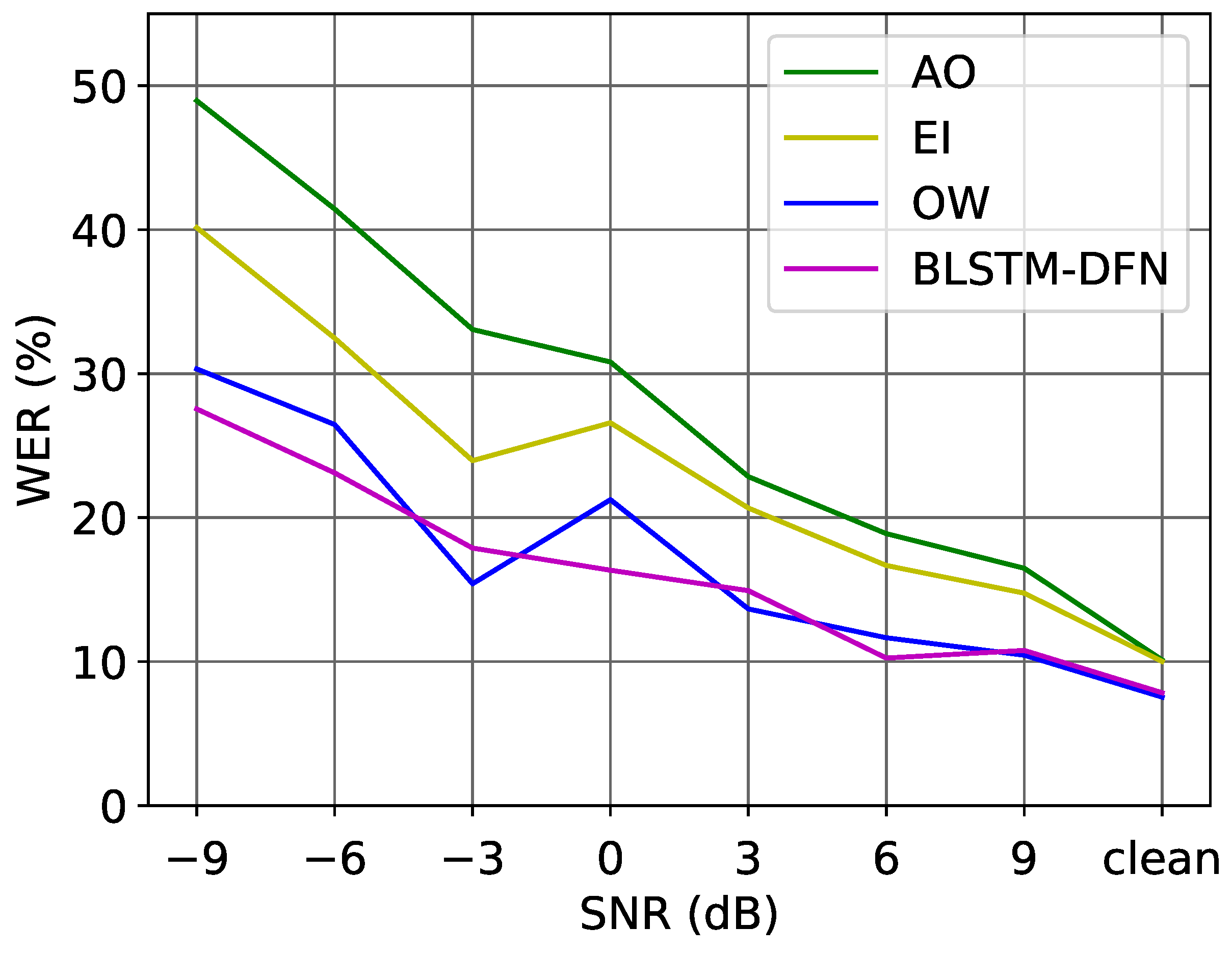
| AO | 48.96 | 41.44 | 33.07 | 30.81 | 22.85 | 18.89 | 16.49 | 10.12 | 27.83 | |
| VA | 85.83 | 87.00 | 85.26 | 88.10 | 87.03 | 88.44 | 88.25 | 88.10 | 87.25 | |
| VS | 88.11 | 90.27 | 87.29 | 88.88 | 85.88 | 85.33 | 88.58 | 87.10 | 87.68 | |
| EI | 40.14 | 32.47 | 23.96 | 26.59 | 20.67 | 16.68 | 14.76 | 10.02 | 23.16 | |
| MSE | 46.48 | 37.79 | 27.45 | 27.47 | 19.52 | 16.58 | 15.09 | 9.42 | 24.98 | |
| CE | 45.79 | 37.14 | 26.32 | 28.03 | 19.40 | 16.68 | 14.76 | 9.42 | 24.65 | |
| OW | 30.33 | 26.47 | 15.41 | 21.25 | 13.66 | 11.66 | 10.45 | 7.54 | 17.10 | |
| LSTM-DFN | 33.30 | 27.22 | 21.26 | 21.25 | 19.17 | 13.97 | 15.84 | 10.32 | 20.29 | |
| BLSTM-DFN | 27.55 | 23.11 | 17.89 | 16.35 | 14.93 | 10.25 | 10.78 | 7.84 | 16.09 | |
| dB | −9 | −6 | −3 | 0 | 3 | 6 | 9 | Clean | Avg. | |
|---|---|---|---|---|---|---|---|---|---|---|
| Model | ||||||||||
| EI | *** | *** | *** | * | ns | ns | ns | ns | *** | |
| MSE | * | *** | *** | ns | * | ** | ** | ns | *** | |
| CE | ns | *** | *** | ns | * | ** | ** | ns | *** | |
| OW | *** | *** | *** | *** | *** | *** | *** | *** | *** | |
| LSTM-DFN | *** | *** | *** | *** | * | *** | ns | ns | *** | |
| BLSTM-DFN | *** | *** | *** | *** | *** | *** | *** | * | *** | |
| AO | EI | MSE | CE | OW | LSTM-DFN | BLSTM-DFN |
|---|---|---|---|---|---|---|
| 23.61 | 19.15 (**) | 19.54 (***) | 19.44 (***) | 12.70 (***) | 15.67 (***) | 15.28 (***) |
| dB | −9 | −6 | −3 | 0 | 3 | 6 | 9 | Clean | Avg. | |
|---|---|---|---|---|---|---|---|---|---|---|
| Model | ||||||||||
| All | 27.55 | 23.11 | 17.89 | 16.35 | 14.93 | 10.25 | 10.78 | 7.84 | 16.09 | |
| 23.39 | 17.96 | 14.51 | 15.68 | 12.97 | 8.44 | 10.67 | 6.94 | 13.82 *** | ||
| 98.12 | 98.50 | 98.76 | 98.22 | 99.43 | 98.79 | 99.46 | 98.81 | 98.76 | ||
| 25.97 | 21.23 | 17.66 | 17.58 | 14.24 | 10.85 | 9.70 | 7.54 | 15.60 | ||
| None | 24.48 | 21.70 | 17.55 | 18.35 | 16.07 | 9.35 | 12.07 | 8.43 | 16.00 | |
| 22.20 | 18.52 | 14.40 | 15.46 | 13.66 | 8.04 | 9.91 | 7.84 | 13.75 *** | ||
| dB | −12 | −9 | −6 | −3 | 0 | 3 | 6 | 9 | 12 | Clean | Avg. | |
|---|---|---|---|---|---|---|---|---|---|---|---|---|
| Model | ||||||||||||
| AO (m) | 18.9 | 13.7 | 11.2 | 8.4 | 6.3 | 6.8 | 4.5 | 4.1 | 4.3 | 4.2 | 8.2 | |
| AO (a) | 25.7 | 23.4 | 18.5 | 11.6 | 8.2 | 9.0 | 5.9 | 3.8 | 4.4 | 4.2 | 11.5 | |
| VO (vc) | 58.7 | 61.0 | 61.7 | 69.6 | 69.6 | 63.5 | 64.6 | 63.6 | 66.6 | 61.9 | 64.1 | |
| VO (gb) | 66.6 | 69.2 | 71.0 | 68.5 | 68.5 | 71.1 | 62.7 | 69.4 | 67.6 | 66.9 | 68.2 | |
| VO (sp) | 68.5 | 72.5 | 73.7 | 70.1 | 70.1 | 70.6 | 68.3 | 69.1 | 73.1 | 67.9 | 70.4 | |
| AV (m.vc) | 14.6 | 11.8 | 6.4 | 7.9 | 7.9 | 6.3 | 5.2 | 4.4 | 3.4 | 4.0 | 7.2 | |
| DFN (m.vc) | 11.1 | 8.7 | 5.5 | 4.8 | 4.8 | 4.5 | 3.6 | 3.3 | 2.2 | 2.4 | 5.1 | |
| AV (a.vc) | 19.1 | 19.0 | 14.3 | 7.3 | 6.3 | 6.0 | 5.7 | 4.5 | 4.9 | 4.0 | 9.1 | |
| DFN (a.vc) | 14.3 | 11.9 | 8.1 | 4.8 | 4.0 | 5.4 | 3.7 | 2.8 | 3.6 | 2.4 | 6.1 | |
| AV (a.gb) | 20.6 | 18.9 | 15.0 | 7.7 | 6.8 | 7.5 | 5.9 | 3.9 | 4.8 | 4.0 | 9.5 | |
| DFN (a.gb) | 14.9 | 12.8 | 9.4 | 5.2 | 4.2 | 5.5 | 3.8 | 3.0 | 4.1 | 2.6 | 6.6 | |
| AV (a.sp) | 19.5 | 19.9 | 15.3 | 7.7 | 7.2 | 6.3 | 5.6 | 4.4 | 4.6 | 4.3 | 9.5 | |
| DFN (a.sp) | 15.4 | 12.8 | 9.9 | 5.2 | 4.7 | 5.5 | 3.4 | 2.6 | 4.0 | 2.5 | 6.6 | |
| dB | −12 | −9 | −6 | −3 | 0 | 3 | 6 | 9 | 12 | Clean | Avg. | |
|---|---|---|---|---|---|---|---|---|---|---|---|---|
| Model | ||||||||||||
| AO-AV (m.vc) | * | ns | *** | ns | ns | ns | ns | ns | ns | ns | *** | |
| AO-DFN (m.vc) | *** | *** | *** | ** | ns | ** | ns | ns | * | *** | *** | |
| AV-DFN (m.vc) | ** | ** | ns | ** | *** | * | ns | * | ns | ** | *** | |
| AO-AV (a.vc) | *** | ** | ** | ** | ns | ** | ns | ns | ns | ns | *** | |
| AO-DFN (a.vc) | *** | *** | *** | *** | *** | *** | ** | ns | ns | *** | *** | |
| AV-DFN (a.vc) | ** | *** | *** | * | * | ns | ** | ns | ns | ** | *** | |
| AO-DFN (a.gb) | *** | *** | *** | *** | *** | *** | * | ns | ns | ** | *** | |
| AV-DFN (a.gb) | *** | *** | *** | * | ** | * | ** | ns | ns | * | *** | |
| AO-DFN (a.sp) | *** | *** | *** | *** | ** | ** | *** | ns | ns | ** | *** | |
| AV-DFN (a.sp) | * | *** | *** | * | * | ns | ** | * | ns | ** | *** | |
| dB | −12 | −9 | −6 | −3 | 0 | 3 | 6 | 9 | 12 | Clean | Avg. | |
|---|---|---|---|---|---|---|---|---|---|---|---|---|
| Model | ||||||||||||
| (m.vc) | 11.2 | 9.4 | 6.5 | 4.3 | 5.4 | 5.5 | 3.6 | 3.1 | 2.3 | 2.4 | 5.4 * | |
| (a.vc) | 14.9 | 14.5 | 10.0 | 6.6 | 4.2 | 5.8 | 4.3 | 2.8 | 2.8 | 2.4 | 6.8 ns | |
| (a.gb) | 16.4 | 14.3 | 10.7 | 6.3 | 4.8 | 6.0 | 4.6 | 3.0 | 2.6 | 2.5 | 7.1 ** | |
| (a.sp) | 17.1 | 15.7 | 11.3 | 6.6 | 4.4 | 6.1 | 4.5 | 2.8 | 2.9 | 2.5 | 7.4 ns | |
| (m.vc) | 10.1 | 8.5 | 6.2 | 5.3 | 5.3 | 5.6 | 3.7 | 3.1 | 2.6 | 2.7 | 5.3 * | |
| (a.vc) | 14.3 | 14.9 | 11.0 | 6.4 | 5.6 | 6.6 | 5.2 | 3.3 | 3.6 | 2.7 | 7.4 | |
| (a.gb) | 16.4 | 15.2 | 11.3 | 6.9 | 4.9 | 6.4 | 4.7 | 3.6 | 3.4 | 2.6 | 7.5 | |
| (a.sp) | 16.1 | 15.0 | 11.4 | 6.6 | 5.3 | 6.1 | 5.1 | 3.1 | 3.4 | 2.5 | 7.5 | |
| None (m.vc) | 11.8 | 8.8 | 6.7 | 7.5 | 6.0 | 5.6 | 3.6 | 3.6 | 3.0 | 3.7 | 6.0 | |
| (a.vc) | 14.9 | 15.2 | 11.3 | 6.0 | 5.2 | 5.9 | 5.6 | 3.8 | 3.3 | 3.7 | 7.5 | |
| (a.gb) | 17.2 | 15.1 | 12.6 | 6.8 | 5.7 | 6.3 | 6.6 | 4.4 | 3.6 | 3.6 | 8.2 | |
| (a.sp) | 16.7 | 16.6 | 12.4 | 6.1 | 6.0 | 5.9 | 5.7 | 3.4 | 3.4 | 3.5 | 8.0 | |
| All (m.vc) | 11.1 | 8.7 | 5.5 | 4.8 | 4.8 | 4.5 | 3.6 | 3.3 | 2.2 | 2.4 | 5.1 ** | |
| (a.vc) | 14.3 | 11.9 | 8.1 | 4.8 | 4.0 | 5.4 | 3.7 | 2.8 | 3.6 | 2.4 | 6.1 *** | |
| (a.gb) | 14.9 | 12.8 | 9.4 | 5.2 | 4.2 | 5.5 | 3.8 | 3.0 | 4.1 | 2.6 | 6.6 *** | |
| (a.sp) | 15.4 | 12.8 | 9.9 | 5.2 | 4.7 | 5.5 | 3.4 | 2.6 | 4.0 | 2.5 | 6.6 *** | |
Publisher’s Note: MDPI stays neutral with regard to jurisdictional claims in published maps and institutional affiliations. |
© 2022 by the authors. Licensee MDPI, Basel, Switzerland. This article is an open access article distributed under the terms and conditions of the Creative Commons Attribution (CC BY) license (https://creativecommons.org/licenses/by/4.0/).
Share and Cite
Yu, W.; Zeiler, S.; Kolossa, D. Reliability-Based Large-Vocabulary Audio-Visual Speech Recognition. Sensors 2022, 22, 5501. https://doi.org/10.3390/s22155501
Yu W, Zeiler S, Kolossa D. Reliability-Based Large-Vocabulary Audio-Visual Speech Recognition. Sensors. 2022; 22(15):5501. https://doi.org/10.3390/s22155501
Chicago/Turabian StyleYu, Wentao, Steffen Zeiler, and Dorothea Kolossa. 2022. "Reliability-Based Large-Vocabulary Audio-Visual Speech Recognition" Sensors 22, no. 15: 5501. https://doi.org/10.3390/s22155501