
IoT and Satellite Sensor Data Integration for Assessment of Environmental Variables: A Case Study on NO2


Abstract
:1. Introduction
- a strong theoretical foundation for modeling the relationship between the IoT and satellite data,
- the integration of interpolation directly into regression models, yielding a more compact and consistent algorithm,
- an ensemble of base regression models constructed by using measurements from the surrounding IoT sensors, and
- an increased temporal resolution, dependent only on the sampling rate of the IoT sensors.
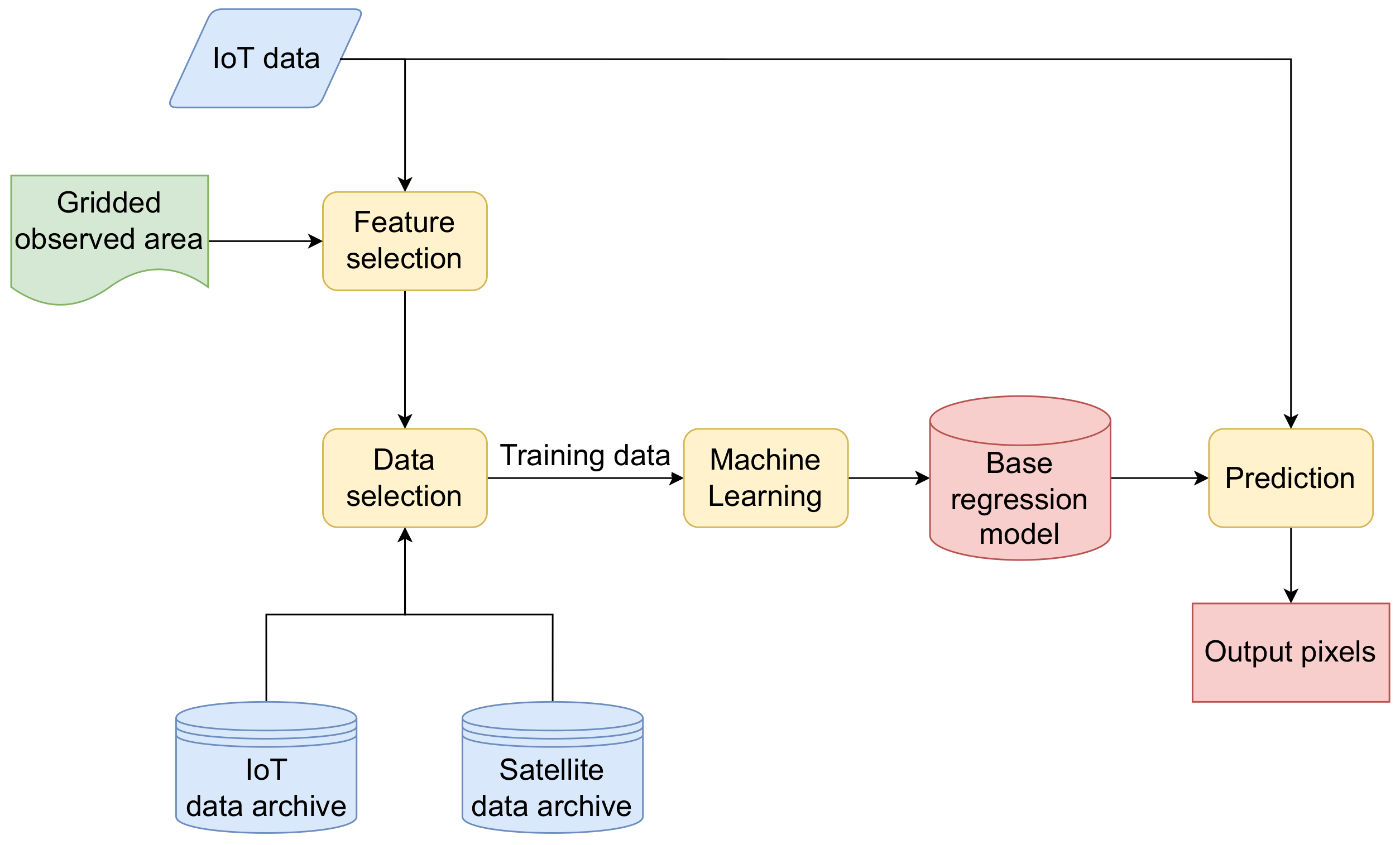
2. Methods
- Feature selection,
- Data selection, and
- Machine learning and Prediction.
2.1. Feature Selection
2.2. Data Selection
Data Selection in Details
2.3. Machine Learning and Prediction
- Nearest Neighbor,
- Linear Regression, and
- Neural Networks.
2.3.1. Nearest Neighbor
2.3.2. Linear Regression
2.3.3. Neural Networks
3. Study Area and Data Preparation
4. Results
5. Discussion
Author Contributions
Funding
Institutional Review Board Statement
Informed Consent Statement
Data Availability Statement
Conflicts of Interest
References
- Gupta, S.; Pebesma, E.; Degbelo, A.; Costa, A.C. Optimising Citizen-Driven Air Quality Monitoring Networks for Cities. ISPRS Int. J. Geo-Inf. 2018, 7, 468. [Google Scholar] [CrossRef] [Green Version]
- Prognostic and Diagnostic Modelling System for Air Pollution Control in the Region. Available online: http://www.kvalitetazraka.si/zasavje/index.php?lang=en (accessed on 4 May 2022).
- Air Quality Data. Available online: https://www.arso.gov.si/en/air/data/ (accessed on 4 May 2022).
- Narayana, M.V.; Jalihal, D.; Shiva Nagendra, S.M. Establishing A Sustainable Low-Cost Air Quality Monitoring Setup: A Survey of the State-of-the-Art. Sensors 2022, 22, 394. [Google Scholar] [CrossRef]
- Kingsy Grace, R.; Manju, S. A Comprehensive Review of Wireless Sensor Networks Based Air Pollution Monitoring Systems. Wirel. Pers. Commun. 2019, 108, 2499–2515. [Google Scholar] [CrossRef]
- Papatsimpa, C.; Linnartz, J.P. Distributed fusion of sensor data in a constrained wireless network. Sensors 2019, 19, 1006. [Google Scholar] [CrossRef] [Green Version]
- Liu, Y.k.; Zhang, X.s.; Zhang, L.; Tao, F.; Wang, L. A multi-agent architecture for scheduling in platform-based smart manufacturing systems. Front. Inform. Technol. Electron. Eng. 2019, 20, 1465–1492. [Google Scholar] [CrossRef]
- Liu, J.; Shi, Y.; Fadlullah, Z.M.; Kato, N. Space-air-ground integrated network: A survey. IEEE Commun. Surv. Tutor. 2018, 20, 2714–2741. [Google Scholar] [CrossRef]
- Agapiou, A.; Lysandrou, V. Observing thermal conditions of historic buildings through earth observation data and big data engine. Sensors 2021, 21, 45571. [Google Scholar] [CrossRef] [PubMed]
- Liang, F.; Gao, M.; Xiao, Q.; Carmichael, G.R.; Pan, X.; Liu, Y. Evaluation of a data fusion approach to estimate daily PM 2.5 levels in North China. Environ. Res. 2017, 158, 54–60. [Google Scholar] [CrossRef] [Green Version]
- Li, J.; Heap, A.D. A Review of Spatial Interpolation Methods for Environmental Scientists; Australian Government: Canberra, Australia, 2008; ISBN 978-19-2149-830-5.
- Manak, M.; Kolingerovà, I. Extension of the edge tracing algorithm to disconnected Voronoi skeletons. Inf. Process. Lett. 2016, 116, 85–92. [Google Scholar] [CrossRef]
- Lee, H.J.; Koutrakis, P. Daily ambient NO2 concentration predictions using satellite ozone monitoring instrument NO2 data and land use regression. Environ. Sci. Technol. 2014, 48, 2305–2311. [Google Scholar] [CrossRef] [PubMed]
- Zhan, Y.; Luo, Y.; Deng, X.; Zhang, K.; Zhang, M.; Grieneisen, M.L.; Di, B. Satellite-Based Estimates of Daily NO2 Exposure in China Using Hybrid Random Forest and Spatiotemporal Kriging Model. Environ. Sci. Technol. 2018, 52, 4180–4189. [Google Scholar] [CrossRef]
- Chen, Z.Y.; Zhang, R.; Zhang, T.H.; Ou, C.Q.; Guo, Y. A kriging-calibrated machine learning method for estimating daily ground-level NO2 in mainland China. Sci. Total. Environ. 2019, 690, 556–564. [Google Scholar] [CrossRef]
- Araki, S.; Shima, M.; Yamamoto, K. Spatiotemporal land use random forest model for estimating metropolitan NO2 exposure in Japan. Sci. Total. Environ. 2018, 634, 1269–1277. [Google Scholar] [CrossRef]
- Huang, W.; Li, T.; Liu, J.; Xie, P.; Du, S.; Teng, F. An overview of air quality analysis by big data techniques: Monitoring, forecasting, and traceability. Inf. Fusion 2021, 75, 28–40. [Google Scholar] [CrossRef]
- Long, M.S.; Yantosca, R.; Nielsen, J.E.; Keller, C.A.; da Silva, A.; Sulprizio, M.P.; Pawson, S.; Jacob, D.J. Development of a grid-independent GEOS-Chem chemical transport model ( v9-02 ) as an atmospheric chemistry module for Earth system models. Geosci. Model. Dev. 2015, 8, 595–602. [Google Scholar] [CrossRef] [Green Version]
- Thongthammachart, T.; Araki, S.; Shimadera, H.; Eto, S.; Matsuo, T.; Kondo, A. An integrated model combining random forests and WRF/CMAQ model for high accuracy spatiotemporal PM2.5 predictions in the Kansai region of Japan. Atmos. Environ. 2021, 262, 118620. [Google Scholar] [CrossRef]
- Li, T.; Wang, Y.; Yuan, Q. Remote sensing estimation of regional NO2 via space-time neural networks. Remote Sens. 2020, 12, 2514. [Google Scholar] [CrossRef]
- Qin, K.; Rao, L.; Xu, J.; Bai, Y.; Zou, J.; Hao, N.; Li, S.; Yu, C. Estimating ground level NO2 concentrations over central-eastern China using a satellite-based geographically and temporally weighted regression model. Remote Sens. 2017, 9, 950. [Google Scholar] [CrossRef] [Green Version]
- Beloconi, A.; Vounatsou, P. Bayesian geostatistical modelling of high-resolution NO2 exposure in Europe combining data from monitors, satellites and chemical transport models. Environ. Int. 2020, 138, 105578. [Google Scholar] [CrossRef]
- Yang, X.; Zheng, Y.; Geng, G.; Liu, H.; Man, H.; Lv, Z.; He, K.; de Hoogh, K. Development of PM2.5 and NO2 models in a LUR framework incorporating satellite remote sensing and air quality model data in Pearl River Delta region, China. Environ. Pollut. 2017, 226, 143–153. [Google Scholar] [CrossRef]
- Di, Q.; Amini, H.; Shi, L.; Kloog, I.; Silvern, R.; Kelly, J.; Sabath, M.B.; Choirat, C.; Koutrakis, P.; Lyapustin, A.; et al. Assessing no2 concentration and model uncertainty with high spatiotemporal resolution across the contiguous united states using ensemble model averaging. Environ. Sci. Technol. 2020, 54, 1372–1384. [Google Scholar] [CrossRef] [PubMed]
- Murray, N.L.; Holmes, H.A.; Liu, Y.; Chang, H.H. A Bayesian ensemble approach to combine PM2.5 estimates from statistical models using satellite imagery and numerical model simulation. Environ. Res. 2019, 178, 108601. [Google Scholar] [CrossRef] [PubMed]
- Wu, X.; Kumar, V. The Top Ten Algorithms in Data Mining; Taylor & Francis Group: New York, NY, USA, 2009; ISBN 978-1-4200-8964-6. [Google Scholar]
- Bai, L.; Wang, J.; Ma, X.; Lu, H. Air pollution forecasts: An overview. Int. J. Environ. Res. Public Health 2018, 15, 780. [Google Scholar] [CrossRef] [PubMed] [Green Version]
- Russell, S.; Norvig, P. Artificial Intelligence A Modern Approach, 4th ed.; Pearson Education: New York, NY, USA, 2021; ISBN 978-013-461-099-3. [Google Scholar]
- Bebis, G.; Georgiopoulos, M. Feed-forward neural networks. IEEE Potentials 1994, 13, 27–31. [Google Scholar] [CrossRef]
- Softmax Function. Available online: https://en.wikipedia.org/wiki/Softmax_function (accessed on 10 May 2022).
- Slovenian Forests. Available online: https://www.tujerodne-vrste.info/en/slovenian-forests/ (accessed on 4 May 2022).
- Infoplease-Slovenia. Available online: https://www.infoplease.com/world/countries/slovenia (accessed on 4 May 2022).
- Slovene sTatistical Regions and Municipalities in Numbers. Available online: https://www.stat.si/obcine/en (accessed on 4 May 2022).
- Maritime Transport. Available online: https://www.gov.si/en/policies/transport-and-energy/maritime-transport/ (accessed on 4 May 2022).
- Port Traffic, Slovenia. 2020. Available online: https://www.stat.si/StatWeb/en/News/Index/9708 (accessed on 4 May 2022).
- TEŠ. Available online: https://www.te-sostanj.si/en/ (accessed on 4 May 2022).
- Sentinel-5P L2. Available online: https://docs.sentinel-hub.com/api/latest/data/sentinel-5p-l2/ (accessed on 4 May 2022).
- Sentinelsat. Available online: https://sentinelsat.readthedocs.io/en/stable/ (accessed on 4 May 2022).
- Sentinel-5 Precursor/TROPOMI Level 2 Product User Manual Nitrogendioxide. Available online: https://sentinel.esa.int/documents/247904/2474726/Sentinel-5P-Level-2-Product-User-Manual-Nitrogen-Dioxide (accessed on 4 May 2022).
- Okolje.Info. Available online: http://www.okolje.info/ (accessed on 4 May 2022).
- MLPACK Linear Regression. Available online: https://mlpack.org/doc/stable/doxygen/classmlpack_1_1regression_1_1LinearRegression.html (accessed on 4 May 2022).
- TensorFlow. Available online: https://www.tensorflow.org/ (accessed on 4 May 2022).
- How to Grid Search Hyperparameters for Deep Learning Models in Python with Keras. Available online: https://machinelearningmastery.com/grid-search-hyperparameters-deep-learning-models-python-keras/ (accessed on 13 June 2022).
- Ripley, B.D. Pattern Recognition and Neural Networks; Cambridge University Press: Cambridge, UK, 1996; ISBN 978-052-146-086-6. [Google Scholar]
- Kuhn, M.; Johnson, K. Applied Predictive Modeling, 1st ed.; Springer: New York, NY, USA, 2013; ISBN 978-146-146-848-6. [Google Scholar]
- Hou, B.J.; Zhang, L.; Zhou, Z.H. Prediction With Unpredictable Feature Evolution. IEEE Trans. Neural Netw. Learn. Syst. 2021, 1–10. [Google Scholar] [CrossRef] [PubMed]
- Sherstinsky, A. Fundamentals of Recurrent Neural Network (RNN) and Long Short-Term Memory (LSTM) network. Phys. D Nonlinear Phenom. 2020, 404, 132306. [Google Scholar] [CrossRef] [Green Version]


| Time | |||||||||
|---|---|---|---|---|---|---|---|---|---|
| ✗ | ✓ | ✓ | ✓ | ✗ | ✗ | ✓ | ✓ | ✗ | |
| ✓ | ✓ | ✗ | ✓ | ✗ | ✓ | ✗ | ✓ | ✓ | |
| ✗ | ✗ | ✗ | ✓ | ✓ | ✗ | ✓ | ✓ | ✓ | |
| ✗ | ✓ | ✓ | ✓ | ✗ | ✗ | ✓ | ✗ | ✗ | |
| ✓ | ✓ | ✗ | ✓ | ✓ | ✗ | ✓ | ✓ | ✓ | |
| ✗ | ✓ | ✓ | ✓ | ✗ | ✓ | ✗ | ✗ | ✗ | |
| ✗ | ✓ | ✗ | ✓ | ✓ | ✓ | ✓ | ✓ | ✓ | |
| ✗ | ✗ | ✗ | ✓ | ✓ | ✗ | ✓ | ✓ | ✓ |
| Time | ||||||||||||||
|---|---|---|---|---|---|---|---|---|---|---|---|---|---|---|
| ✓ | ✓ | ✓ | ✓ | ✓ | ✗ | ✓ | ✓ | ✓ | ✗ | ✓ | ✓ | … | ✗ | |
| ✓ | ✗ | ✓ | ✓ | ✗ | ✓ | ✓ | ✗ | ✓ | ✗ | ✗ | ✗ | … | ✓ | |
| ✓ | ✓ | ✓ | ✓ | ✓ | ✓ | ✓ | ✗ | ✓ | ✓ | ✓ | ✗ | … | ✗ | |
| ✗ | ✓ | ✗ | ✗ | ✗ | ✓ | ✗ | ✓ | ✗ | ✓ | ✓ | ✓ | … | ✗ | |
| ✓ | ✓ | ✓ | ✓ | ✓ | ✓ | ✓ | ✓ | ✓ | ✗ | ✗ | ✓ | … | ✓ | |
| ✗ | ✓ | ✓ | ✗ | ✓ | ✓ | ✗ | ✓ | ✓ | ✓ | ✓ | ✓ | … | ✗ | |
| ✗ | ✓ | ✗ | ✗ | ✗ | ✓ | ✗ | ✓ | ✗ | ✗ | ✓ | ✗ | … | ✗ | |
| ✓ | ✓ | ✗ | ✓ | ✗ | ✓ | ✓ | ✓ | ✗ | ✓ | ✓ | ✓ | … | ✓ |
| BRM | 1-NN | LR | NN | |||
|---|---|---|---|---|---|---|
| Area | RMSE () | Execution Times * [] | RMSE () | Execution Time * [] | RMSE () | Execution Time * [] |
| Test case 1 | 24.13 | 1 | 22.63 | 7 | 18.95 | 2 |
| Test case 2 | 22.18 | 2 | 20.19 | 6 | 17.05 | 3 |
| Test case 3 | 24.26 | 2 | 21.25 | 7 | 19.53 | 4 |
| Test case 4 | 23.35 | 6 | 19.99 | 7 | 18.58 | 3 |
| Test case 5 | 22.68 | 1 | 19.15 | 7 | 17.75 | 2 |
| Test case 6 | 22.77 | 12 | 18.87 | 8 | 17.67 | 4 |
| Test case 7 | 22.98 | 7 | 18.66 | 7 | 17.70 | 1 |
| Test case 8 | 23.13 | 4 | 18.36 | 6 | 17.46 | 1 |
| Whole | 21.82 | 43 | 16.95 | 8 | 15.49 | 14 |
| Test Case–RMSE () | ||||||||
|---|---|---|---|---|---|---|---|---|
| Number * | 1 | 2 | 3 | 4 | 5 | 6 | 7 | 8 |
| 3 | 55.19 | / | / | / | / | 28.93 | / | / |
| 4 | 16.50 | 12.08 | 20.94 | / | 10.60 | 17.90 | 10.57 | 11.65 |
| 5 | 19.25 | 10.45 | 28.72 | 11.61 | 18.79 | 16.81 | 14.10 | 18.98 |
| 6 | 12.82 | 13.94 | 21.25 | 15.06 | 13.93 | 17.07 | 18.78 | / |
| 7 | / | / | 20.28 | 16.70 | 11.49 | 17.40 | / | / |
| 8 | / | 2.419 | 25.48 | 14.62 | / | 17.19 | / | / |
| 9 | / | / | / | / | / | 16.66 | / | / |
| Test Case–Average Distance [km] | ||||||||
|---|---|---|---|---|---|---|---|---|
| Number * | 1 | 2 | 3 | 4 | 5 | 6 | 7 | 8 |
| 3 | 60.42 | / | / | / | / | 1.51 | / | / |
| 4 | 80.89 | 76.86 | 23.85 | / | 44.53 | 2.95 | 47.49 | 60.60 |
| 5 | 81.73 | 80.96 | 33.79 | 28.24 | 49.24 | 19.18 | 47.89 | 82.24 |
| 6 | 96.07 | 80.57 | 38.49 | 33.55 | 56.38 | 17.20 | 48.18 | / |
| 7 | / | / | 30.91 | 35.68 | 62.99 | 19.81 | / | / |
| 8 | / | 93.71 | 40.69 | 38.71 | / | 44.12 | / | / |
| 9 | / | / | / | / | / | 47.21 | / | / |
| Considered Variable | Temperature | Wind Speed | Wind Direction | Humidity | |
|---|---|---|---|---|---|
| Test case–RMSE () | 16.29 | 17.27 | 17.71 | 17.60 | 15.47 |
Publisher’s Note: MDPI stays neutral with regard to jurisdictional claims in published maps and institutional affiliations. |
© 2022 by the authors. Licensee MDPI, Basel, Switzerland. This article is an open access article distributed under the terms and conditions of the Creative Commons Attribution (CC BY) license (https://creativecommons.org/licenses/by/4.0/).
Share and Cite
Cukjati, J.; Mongus, D.; Žalik, K.R.; Žalik, B. IoT and Satellite Sensor Data Integration for Assessment of Environmental Variables: A Case Study on NO2. Sensors 2022, 22, 5660. https://doi.org/10.3390/s22155660
Cukjati J, Mongus D, Žalik KR, Žalik B. IoT and Satellite Sensor Data Integration for Assessment of Environmental Variables: A Case Study on NO2. Sensors. 2022; 22(15):5660. https://doi.org/10.3390/s22155660
Chicago/Turabian StyleCukjati, Jernej, Domen Mongus, Krista Rizman Žalik, and Borut Žalik. 2022. "IoT and Satellite Sensor Data Integration for Assessment of Environmental Variables: A Case Study on NO2" Sensors 22, no. 15: 5660. https://doi.org/10.3390/s22155660
APA StyleCukjati, J., Mongus, D., Žalik, K. R., & Žalik, B. (2022). IoT and Satellite Sensor Data Integration for Assessment of Environmental Variables: A Case Study on NO2. Sensors, 22(15), 5660. https://doi.org/10.3390/s22155660