
Comparison of Correlation between 3D Surface Roughness and Laser Speckle Pattern for Experimental Setup Using He-Ne as Laser Source and Laser Pointer as Laser Source


Abstract
:1. Introduction
2. Materials and Methods
2.1. Sample Preparation
- Arithmetic mean height (Sa);
- Root-mean-square height (Sq);
- Maximum peak height (Sp);
- Maximum valley depth (Sv);
- Maximum height (Sz);
- Ten point height (S10z);
- Skewness (Ssk);
- Kurtosis (Sku);
- Root-mean-square gradient (Sdq);
- Developed interfacial area ratio (Sdr).
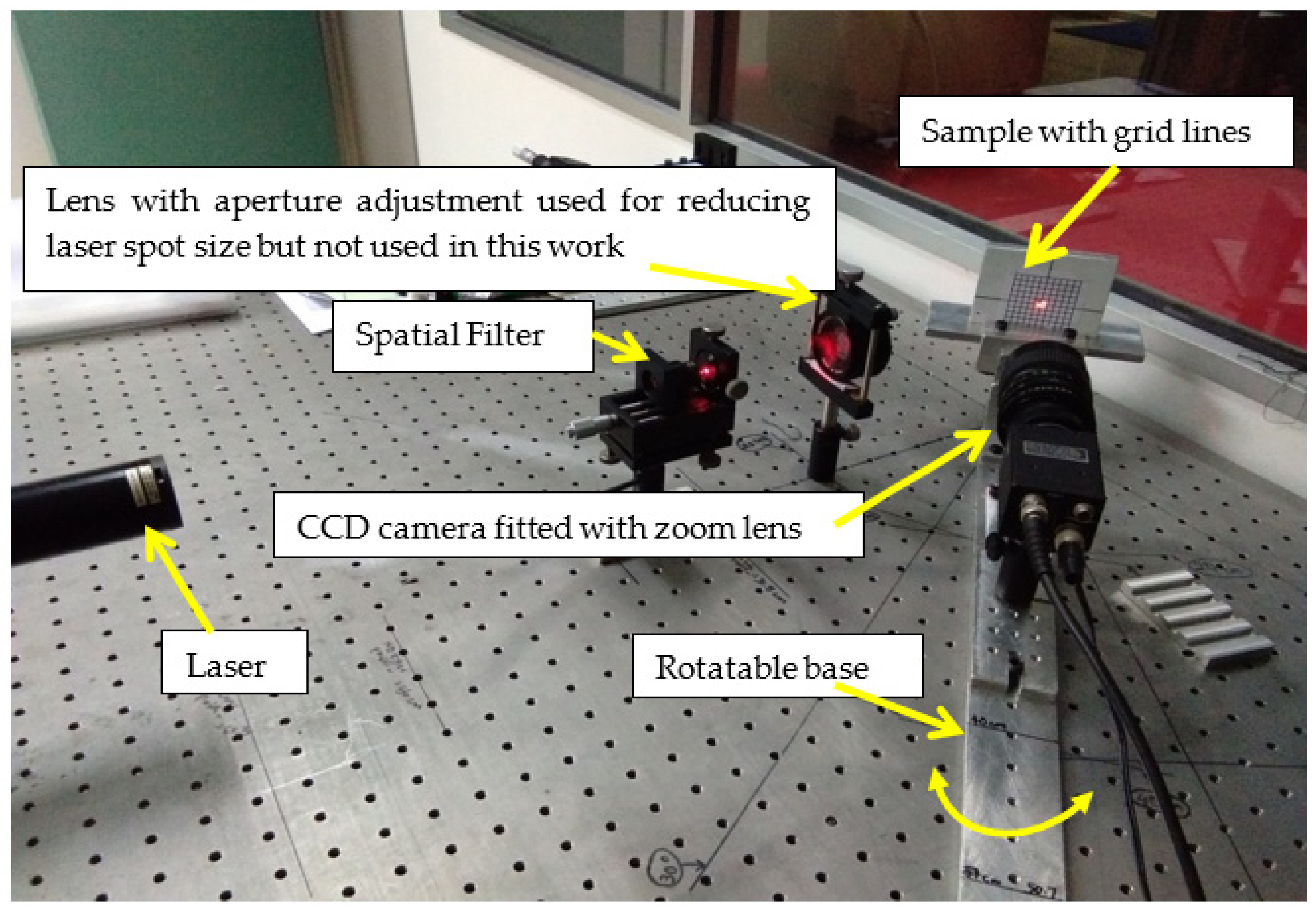
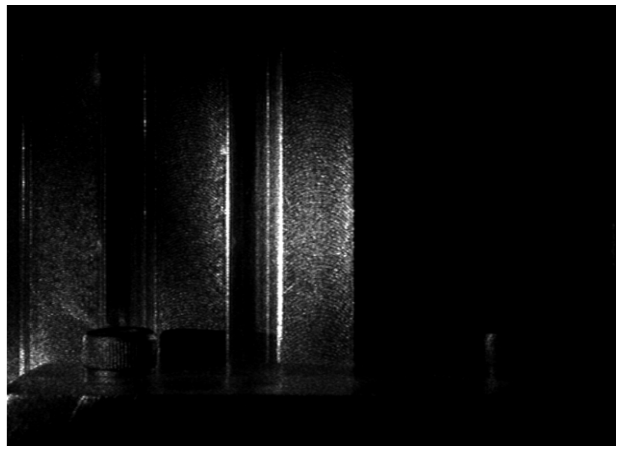
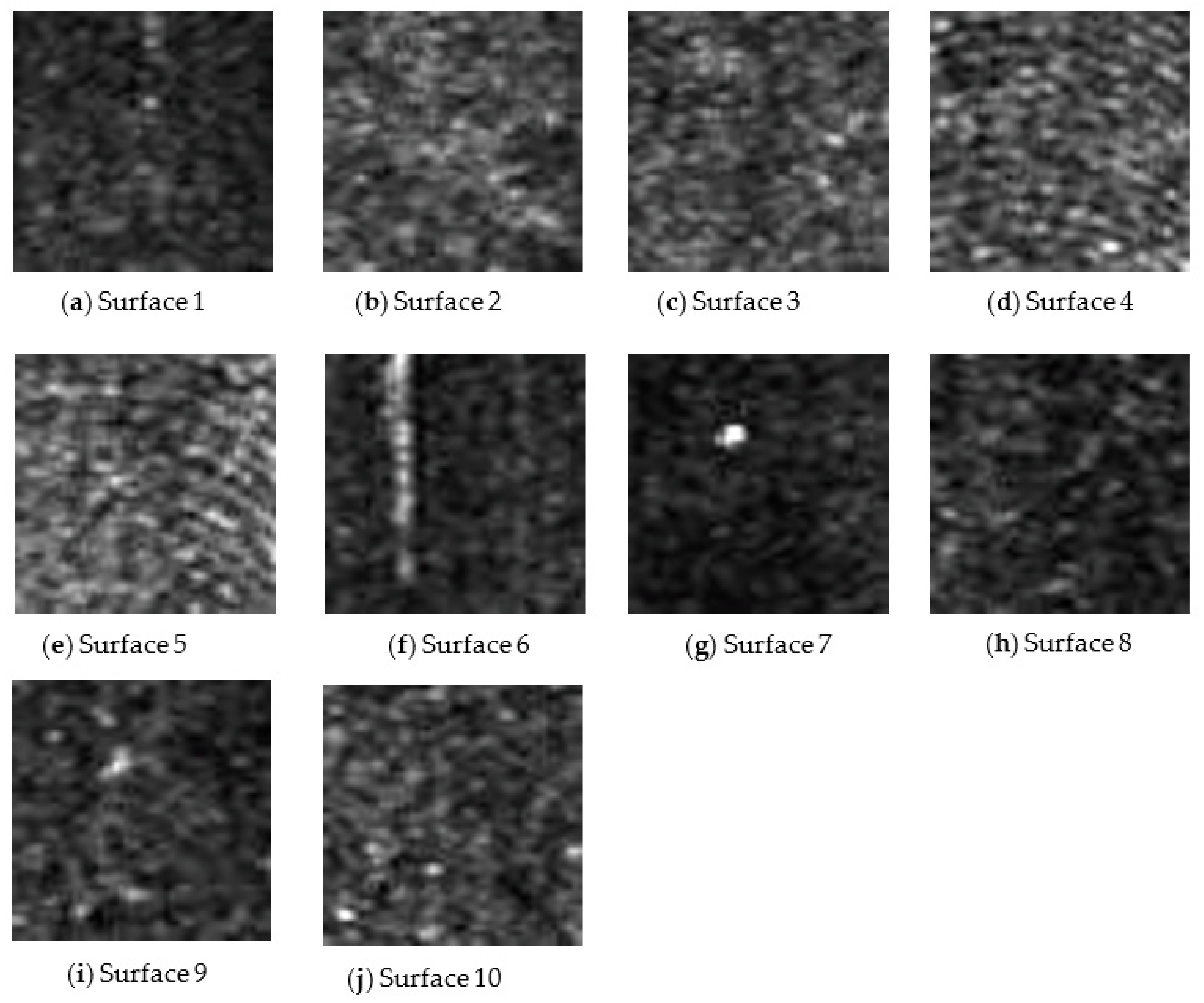
2.2. Experimental Setup 1
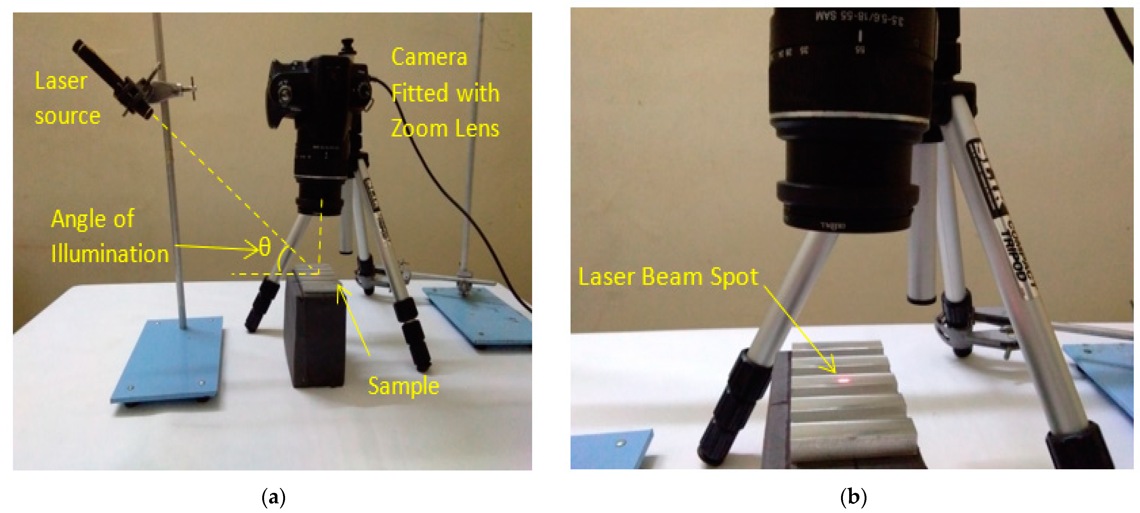
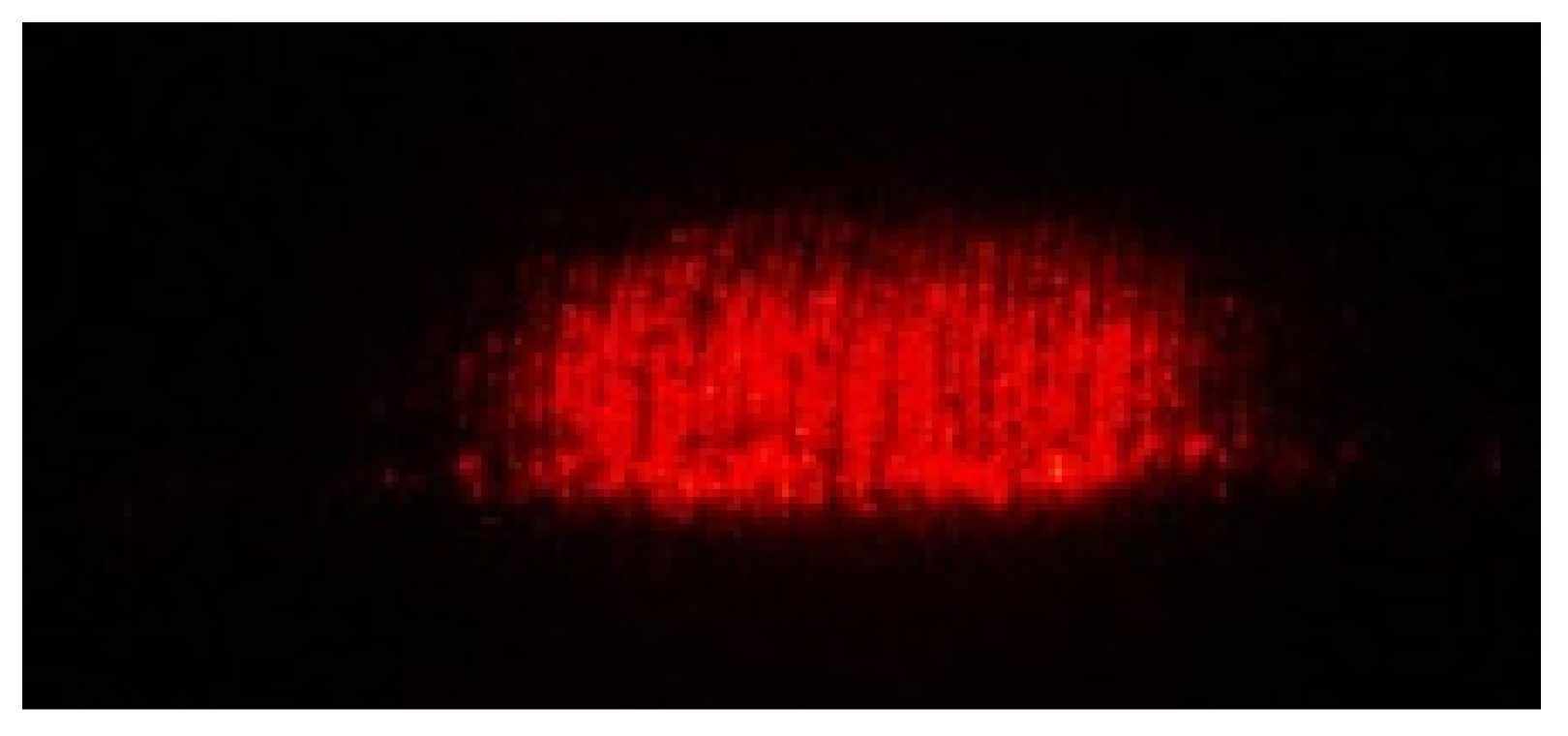
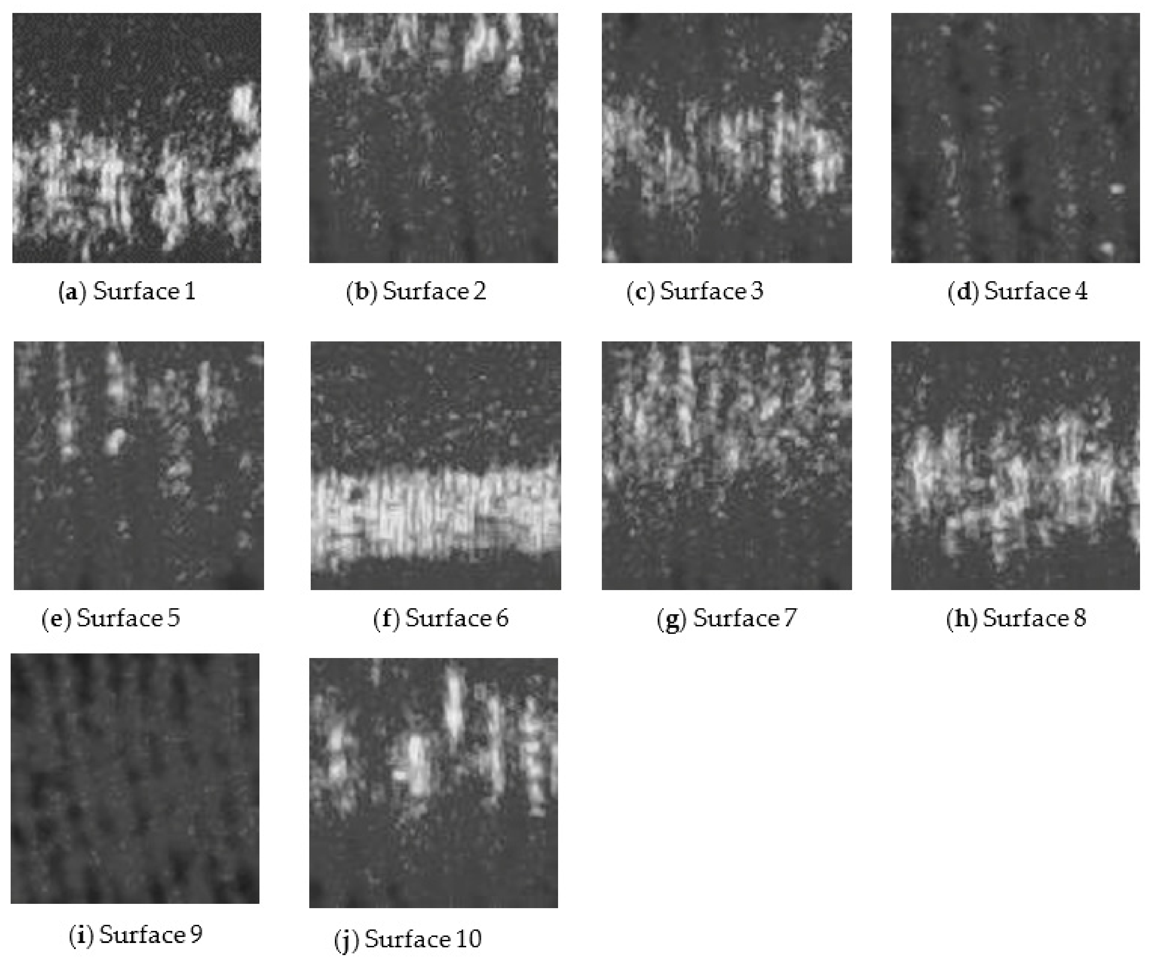
2.3. Experimental Setup 2
2.4. Characteristic Features Extraction
- Histogram-based (statistical) features
- ○
- Mean
- ○
- Standard deviation
- rj is the jth gray level;
- L is the total possible gray level value;
- p(rj) is the probability of occurrences of rj;
- m is the mean of gray values of the image.
- ○
- Energy
- rj is the jth gray level;
- L is the total possible gray level value;
- p(rj) is the probability of occurrences of rj.
- ○
- Entropy
- rj is the jth gray level;
- L is the total possible gray level value;
- p(rj) is the probability of occurrences of rj.
- Texture features
- ○
- The normalised descriptor of roughness
- σ2 is variance;
- L is the total possible gray level value.
- Gray level co-occurrence matrix (GLCM)
- Ng(i,j) is the normalized gray level co-occurrence matrix;
- g(i,j) is the element of the gray level co-occurrence matrix.
- ○
- Maximum probability (GLCM) is given by Equation (7).
- ○
- Correlation (GLCM) is given by Equation (8).
- µi is the mean of the row sums of Ng(i,j);
- µj is the mean of column sums of Ng(i,j);
- σi is the standard deviation of row sums of Ng(i,j);
- σj is the standard deviation of column sums of Ng(i,j).
- ○
- Contrast (GLCM) is given by Equation (9).
- ○
- Energy (GLCM) is given by Equation (10).
- ○
- Homogeneity (GLCM) is given by Equation (11).
- ○
- Entropy (GLCM) is given by Equation (12).
- From the binary image, the following characteristic features were extracted:
- ○
- Total white pixels to total black pixels ratio (W/B).
3. Results and Discussion
4. Conclusions
Author Contributions
Funding
Institutional Review Board Statement
Informed Consent Statement
Data Availability Statement
Acknowledgments
Conflicts of Interest
References
- Degarmo, E.P.; Black, J.T.; Kohser, R.A. Materials and Processess in Manufacturing, 8th ed.; Prentice-Hall International: Upper Saddle River, NJ, USA, 1997; p. 288. [Google Scholar]
- Liu, J.; Lu, E.; Yi, H.; Wang, M.; Ao, P. A new surface roughness measurement method based on a color distribution statistical matrix. Measurement 2017, 103, 165–178. [Google Scholar] [CrossRef]
- Rifai, A.P.; Aoyama, H.; Tho, N.H.; Md Dawal, S.Z.; Masruroh, N.A. Evaluation of turned and milled surfaces roughness using convolutional neural network. Measurement 2020, 161, 107860. [Google Scholar] [CrossRef]
- Agrawal, A.; Goel, S.; Rashid, W.B.; Price, M. Prediction of surface roughness during hard turning of AISI 4340 steel (69 HRC). Appl. Soft Comput. 2015, 30, 279–286. [Google Scholar] [CrossRef]
- Manojlovic, L.M.; Zivanov, M.B.; Marincic, A.S. White-Light Interferometric Sensor for Rough Surface Height Distribution Measurement. IEEE Sens. J. 2010, 10, 1125–1132. [Google Scholar] [CrossRef]
- Petzold, S.; Klett, J.; Schauer, A.; Osswald, T.A. Surface roughness of polyamide 12 parts manufactured using selective laser sintering. Polym. Test. 2019, 80, 106094. [Google Scholar] [CrossRef]
- Tsigarida, A.; Tsampali, E.; Konstantinidis, A.A.; Stefanidou, M. On the use of confocal microscopy for calculating the surface microroughness and the respective hydrophobic properties of marble specimens. J. Build. Eng. 2021, 33, 101876. [Google Scholar] [CrossRef]
- Goh, C.S.; Ratnam, M.M. Assessment of Areal (Three-Dimensional) Roughness Parameters of Milled Surface Using Charge-Coupled Device Flatbed Scanner and Image Processing. Exp. Tech. 2016, 40, 1099–1107. [Google Scholar] [CrossRef]
- Xu, D.; Yang, Q.; Dong, F.; Krishnaswamy, S. Evaluation of surface roughness of a machined metal surface based on laser speckle pattern. J. Eng. 2018, 2018, 773–778. [Google Scholar] [CrossRef]
- Jayabarathi, S.B.; Ratnam, M.M. Correlation Study of 3D Surface Roughness of Milled Surfaces with Laser Speckle Pattern. Sensors 2022, 22, 2842. [Google Scholar] [CrossRef]
- Mahashar, A.J.; Siddhi, J.H.; Murugan, M. Surface roughness evaluation of electrical discharge machined surfaces using wavelet transform of speckle line images. Measurement 2020, 149, 107029. [Google Scholar] [CrossRef]
- Soares, H.C.; Meireles, J.B.; Castro, A.O.; Huguenin, J.A.O.; Schmidt, A.G.M.; da Silva, L. Tsallis threshold analysis of digital speckle patterns generated by rough surfaces. Phys. A Stat. Mech. Appl. 2015, 432, 1–8. [Google Scholar] [CrossRef]
- Joshi, K.; Patil, B. Prediction of Surface Roughness by Machine Vision using Principal Components based Regression Analysis. Procedia Comput. Sci. 2020, 167, 382–391. [Google Scholar] [CrossRef]
- Dias, M.R.B.; Dornelas, D.; Balthazar, W.F.; Huguenin, J.A.O.; da Silva, L. Lacunarity study of speckle patterns produced by rough surfaces. Phys. A Stat. Mech. Appl. 2017, 486, 328–336. [Google Scholar] [CrossRef]
- Baradit, E.; Gatica, C.; Yáñez, M.; Figueroa, J.C.; Guzmán, R.; Catalán, C. Surface roughness estimation of wood boards using speckle interferometry. Opt. Lasers Eng. 2020, 128, 106009. [Google Scholar] [CrossRef]
- Goch, G.; Peters, J.; Lehmann, P.; Liu, H. Requirements for the Application of Speckle Correlation Techniques to On-Line Inspection of Surface Roughness. CIRP Ann. 1999, 48, 467–470. [Google Scholar] [CrossRef]
- Dhanasekar, B.; Mohan, N.K.; Bhaduri, B.; Ramamoorthy, B. Evaluation of surface roughness based on monochromatic speckle correlation using image processing. Precis. Eng. 2008, 32, 196–206. [Google Scholar] [CrossRef]
- Toh, S.L.; Shang, H.M.; Tay, C.J. Surface-roughness study using laser speckle method. Opt. Lasers Eng. 1998, 29, 217–225. [Google Scholar] [CrossRef]
- Tchvialeva, L.; Markhvida, I.; Zeng, H.; McLean, D.I.; Lui, H.; Lee, T.K. Surface roughness measurement by speckle contrast under the illumination of light with arbitrary spectral profile. Opt. Lasers Eng. 2010, 48, 774–778. [Google Scholar] [CrossRef]
- Leonard, L.C.; Toal, V. Roughness measurement of metallic surfaces based on the laser speckle contrast method. Opt. Lasers Eng. 1998, 30, 433–440. [Google Scholar] [CrossRef]
- Smith, G.T. Industrial Metrology: Surfaces and Roundness; Springer: London, UK, 2002. [Google Scholar]
- Wang, T.; Xie, L.-j.; Wang, X.-b.; Shang, T.-y. 2D and 3D milled surface roughness of high volume fraction SiCp/Al composites. Def. Technol. 2015, 11, 104–109. [Google Scholar] [CrossRef]
- Molnár, V. Minimization Method for 3D Surface Roughness Evaluation Area. Machines 2021, 9, 192. [Google Scholar] [CrossRef]
- Zhang, X.; Zheng, Y.; Suresh, V.; Wang, S.; Li, Q.; Li, B.; Qin, H. Correlation approach for quality assurance of additive manufactured parts based on optical metrology. J. Manuf. Processes 2020, 53, 310–317. [Google Scholar] [CrossRef]
- Fuji, H.; Asakura, T.; Shindo, Y. Measurement of surface roughness properties by means of laser speckle techniques. Opt. Commun. 1976, 16, 68–72. [Google Scholar] [CrossRef]
- ISO 25178-2:2012; Geometrical Product Specifications (GPS)—Surface Texture: Areal—Part 2: Terms, Definitions and Surface Texture Parameters. ISO: Geneva, Switzerland, 2012.
- Marques, O. Practical Image and Video Processing using MATLAB; John Wiley & Sons: Hoboken, NJ, USA, 2011. [Google Scholar]


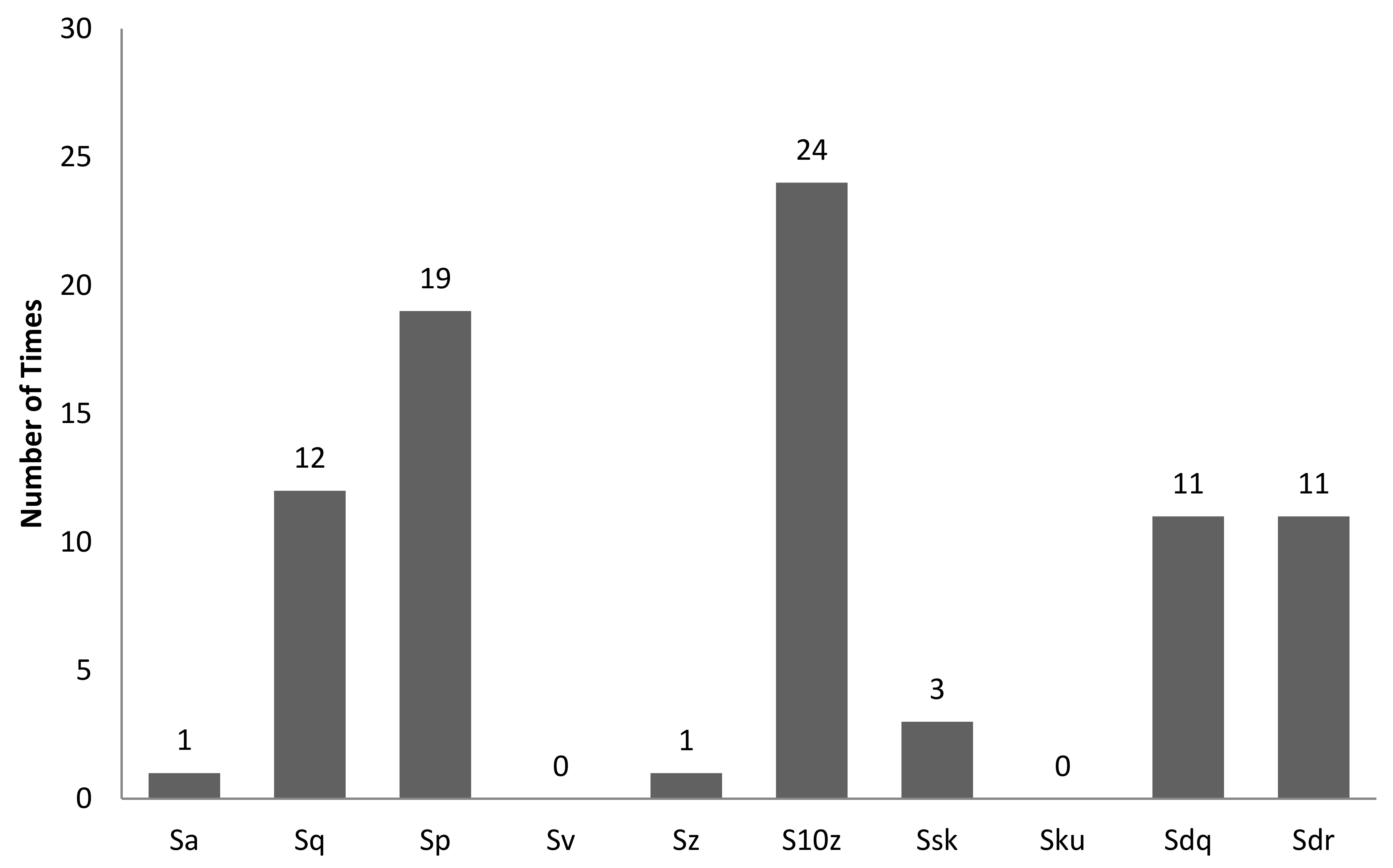
| Surface No. | Spindle Speed (rpm) | Feed Rate (mm/min) | Depth of Cut (mm) | Sa (µm) | Sq (µm) | Sp (µm) | Sv (µm) | Sz (µm) | S10z (µm) | Ssk | Sku | Sdq | Sdr (%) |
|---|---|---|---|---|---|---|---|---|---|---|---|---|---|
| 1 | 1000 | 120 | 1 | 0.931 | 1.117 | 4.070 | 3.889 | 7.959 | 6.187 | −0.044 | 2.415 | 0.161 | 1.305 |
| 2 | 1000 | 280 | 1 | 1.046 | 1.322 | 8.081 | 7.774 | 15.855 | 9.217 | 0.281 | 3.398 | 0.177 | 1.553 |
| 3 | 1000 | 440 | 1 | 1.325 | 1.675 | 9.809 | 6.795 | 16.605 | 10.826 | 0.146 | 3.442 | 0.191 | 1.790 |
| 4 | 1000 | 600 | 1 | 1.162 | 1.567 | 11.639 | 13.136 | 24.775 | 14.423 | 0.275 | 6.054 | 0.242 | 2.636 |
| 5 | 1000 | 760 | 1 | 1.254 | 1.816 | 10.948 | 8.678 | 19.626 | 16.608 | 0.360 | 6.142 | 0.318 | 4.565 |
| 6 | 2500 | 120 | 1 | 0.748 | 0.902 | 5.681 | 6.960 | 12.641 | 5.122 | 0.335 | 2.473 | 0.185 | 1.722 |
| 7 | 2500 | 280 | 1 | 0.968 | 1.156 | 5.437 | 8.607 | 14.045 | 6.387 | −0.177 | 6.528 | 0.185 | 1.749 |
| 8 | 2500 | 440 | 1 | 0.974 | 1.225 | 7.169 | 6.327 | 13.496 | 7.440 | −0.124 | 4.374 | 0.196 | 1.830 |
| 9 | 2500 | 600 | 1 | 1.058 | 1.326 | 8.617 | 9.490 | 18.106 | 8.325 | 0.000 | 3.152 | 0.192 | 1.888 |
| 10 | 2500 | 760 | 1 | 1.113 | 1.417 | 9.640 | 6.377 | 16.016 | 10.246 | 0.257 | 3.715 | 0.193 | 1.811 |
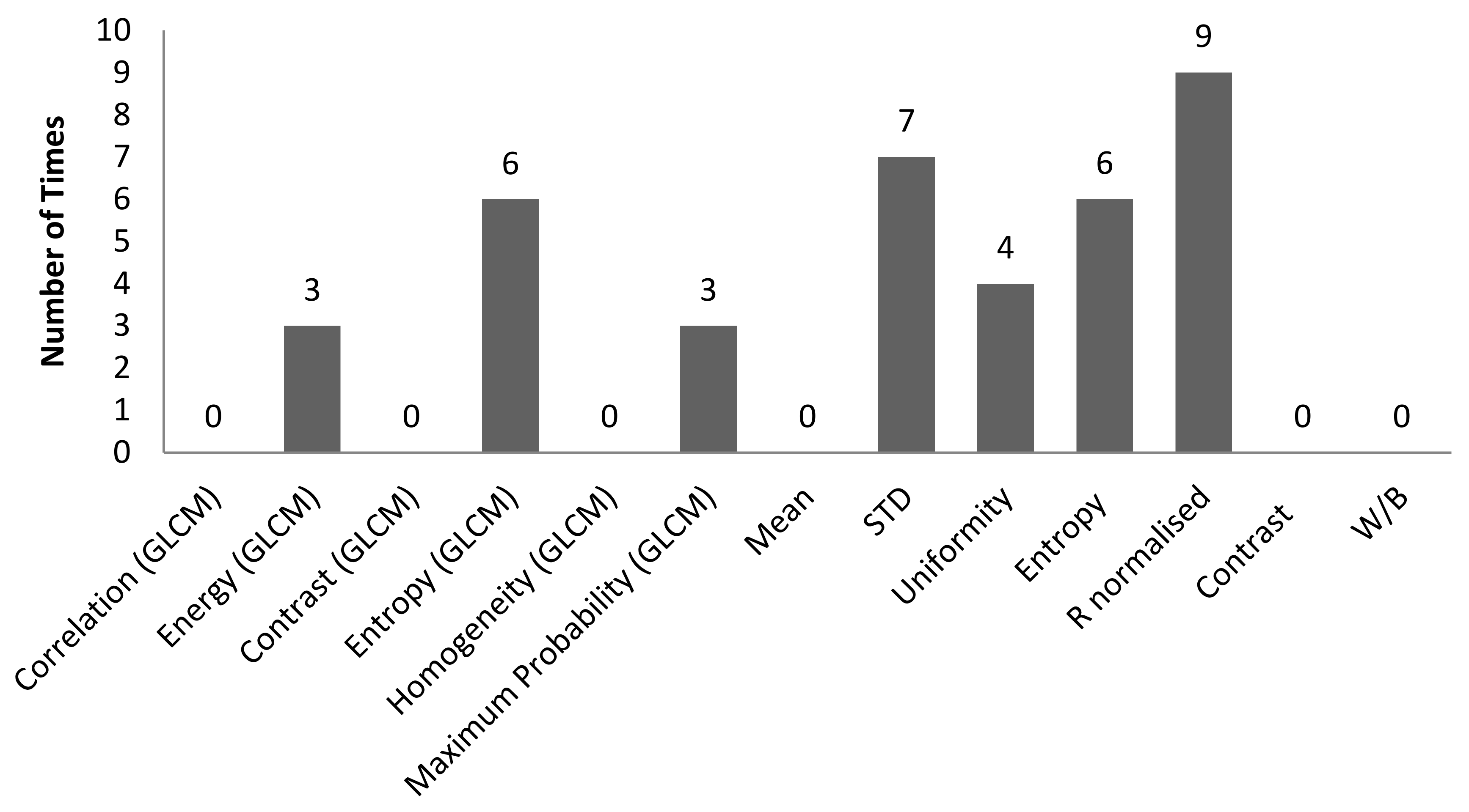
| Characteristic Features | 3D Surface Roughness Parameters | |||||||||
|---|---|---|---|---|---|---|---|---|---|---|
| Sa | Sq | Sp | Sv | Sz | S10z | Ssk | Sku | Sdq | Sdr | |
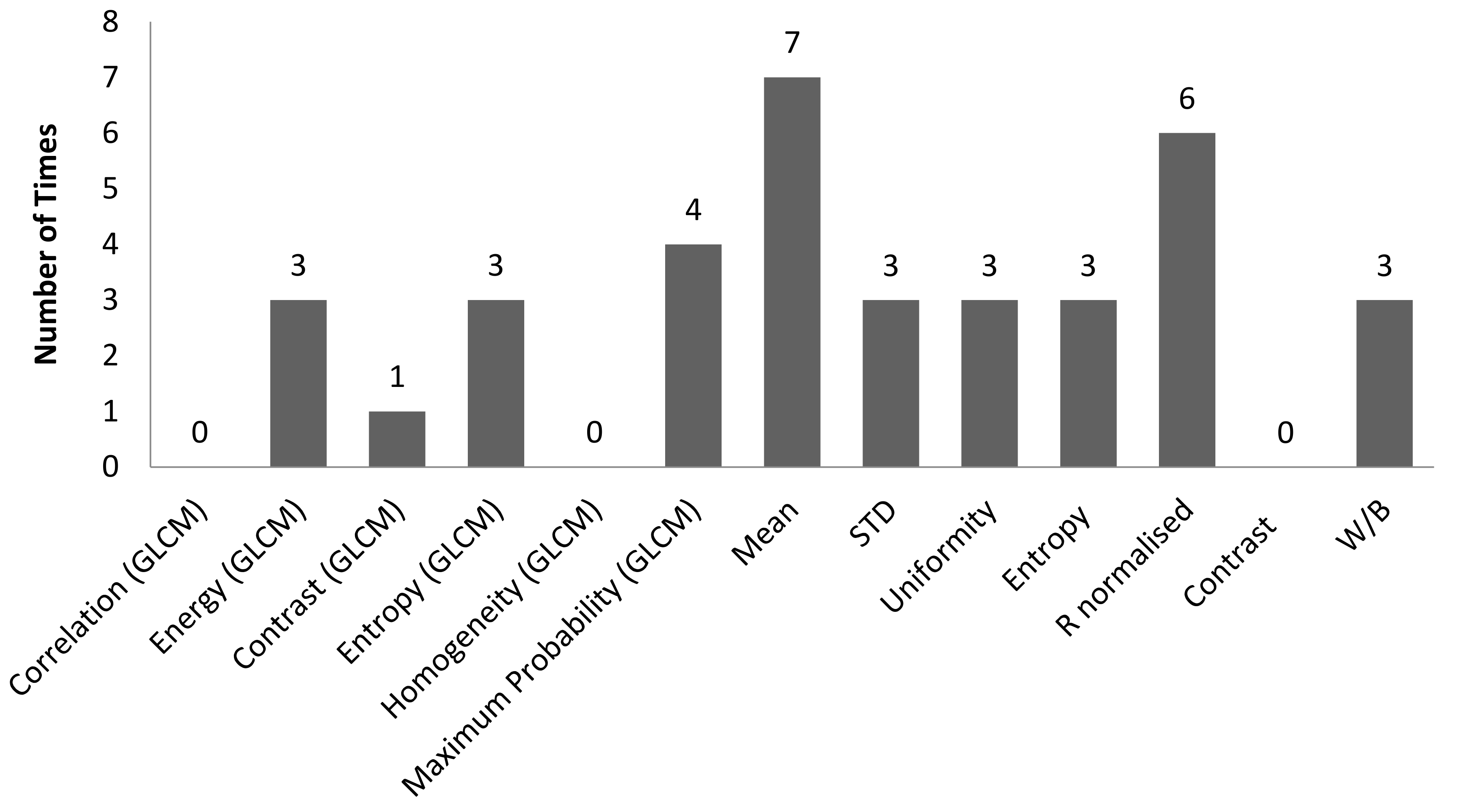
| Correlation (GLCM). | ||||||||||
| Energy (GLCM) | 1 | 1 | 1 | |||||||
| Contrast (GLCM) | ||||||||||
| Entropy (GLCM) | 1 | 3 | 2 | |||||||
| Homogeneity (GLCM) | ||||||||||
| Maximum probability (GLCM) | 1 | 1 | 1 | |||||||
| Mean | ||||||||||
| STD | 1 | 4 | 1 | 1 | ||||||
| Uniformity | 1 | 1 | 2 | |||||||
| Entropy | 1 | 3 | 2 | |||||||
| R normalised | 1 | 4 | 2 | 2 | ||||||
| Contrast | ||||||||||
| W/B | ||||||||||
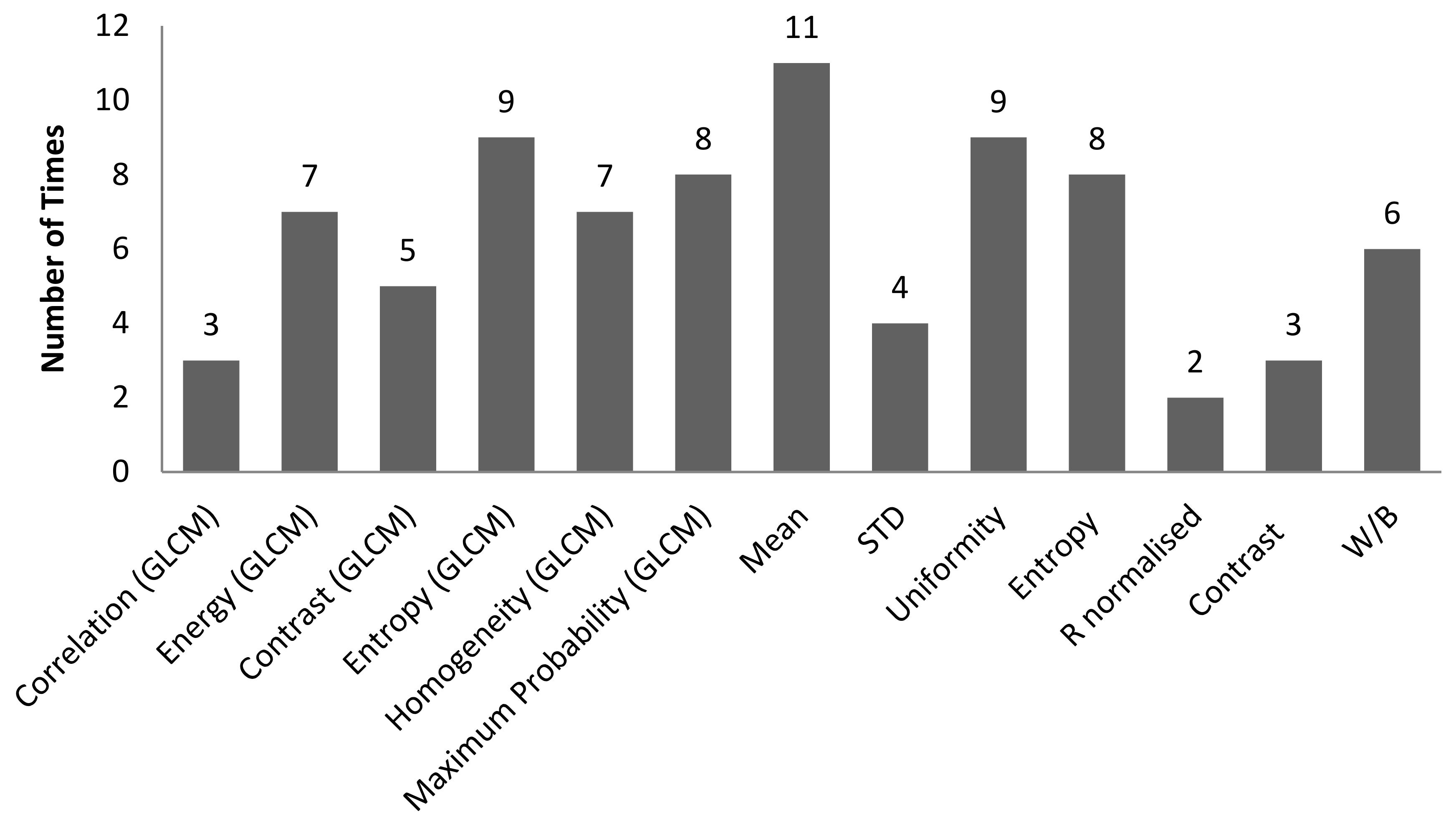
| Characteristic Features | 3D Surface Roughness Parameters | |||||||||
|---|---|---|---|---|---|---|---|---|---|---|
| Sa | Sq | Sp | Sv | Sz | S10z | Ssk | Sku | Sdq | Sdr | |
| Correlation (GLCM) | ||||||||||
| Energy (GLCM) | 1 | 1 | 1 | |||||||
| Contrast (GLCM) | 1 | |||||||||
| Entropy (GLCM) | 1 | 2 | ||||||||
| Homogeneity (GLCM) | ||||||||||
| Maximum probability (GLCM) | 1 | 1 | 1 | 1 | ||||||
| Mean | 2 | 1 | 4 | |||||||
| STD | 1 | 2 | ||||||||
| Uniformity | 1 | 2 | ||||||||
| Entropy | 1 | 2 | ||||||||
| R normalised | 1 | 2 | 2 | 1 | ||||||
| Contrast | ||||||||||
| W/B | 1 | 1 | 1 | |||||||
| Characteristic Features | 3D Surface Roughness Parameters | |||||||||
|---|---|---|---|---|---|---|---|---|---|---|
| Sa | Sq | Sp | Sv | Sz | S10z | Ssk | Sku | Sdq | Sdr | |
| Correlation (GLCM) | 1 | 1 | 1 | |||||||
| Energy (GLCM) | 1 | 2 | 2 | 1 | 1 | |||||
| Contrast (GLCM) | 1 | 1 | 1 | 1 | 1 | |||||
| Entropy (GLCM) | 1 | 3 | 3 | 1 | 1 | |||||
| Homogeneity (GLCM) | 2 | 1 | 2 | 1 | 1 | |||||
| Maximum probability (GLCM) | 1 | 3 | 1 | 1 | 1 | 1 | ||||
| Mean | 2 | 4 | 3 | 1 | 1 | |||||
| STD | 1 | 1 | 2 | |||||||
| Uniformity | 1 | 2 | 3 | 1 | 1 | 1 | ||||
| Entropy | 1 | 3 | 3 | 1 | ||||||
| R normalised | 1 | 1 | ||||||||
| Contrast | 1 | 1 | 1 | |||||||
| W/B | 2 | 2 | 2 | |||||||
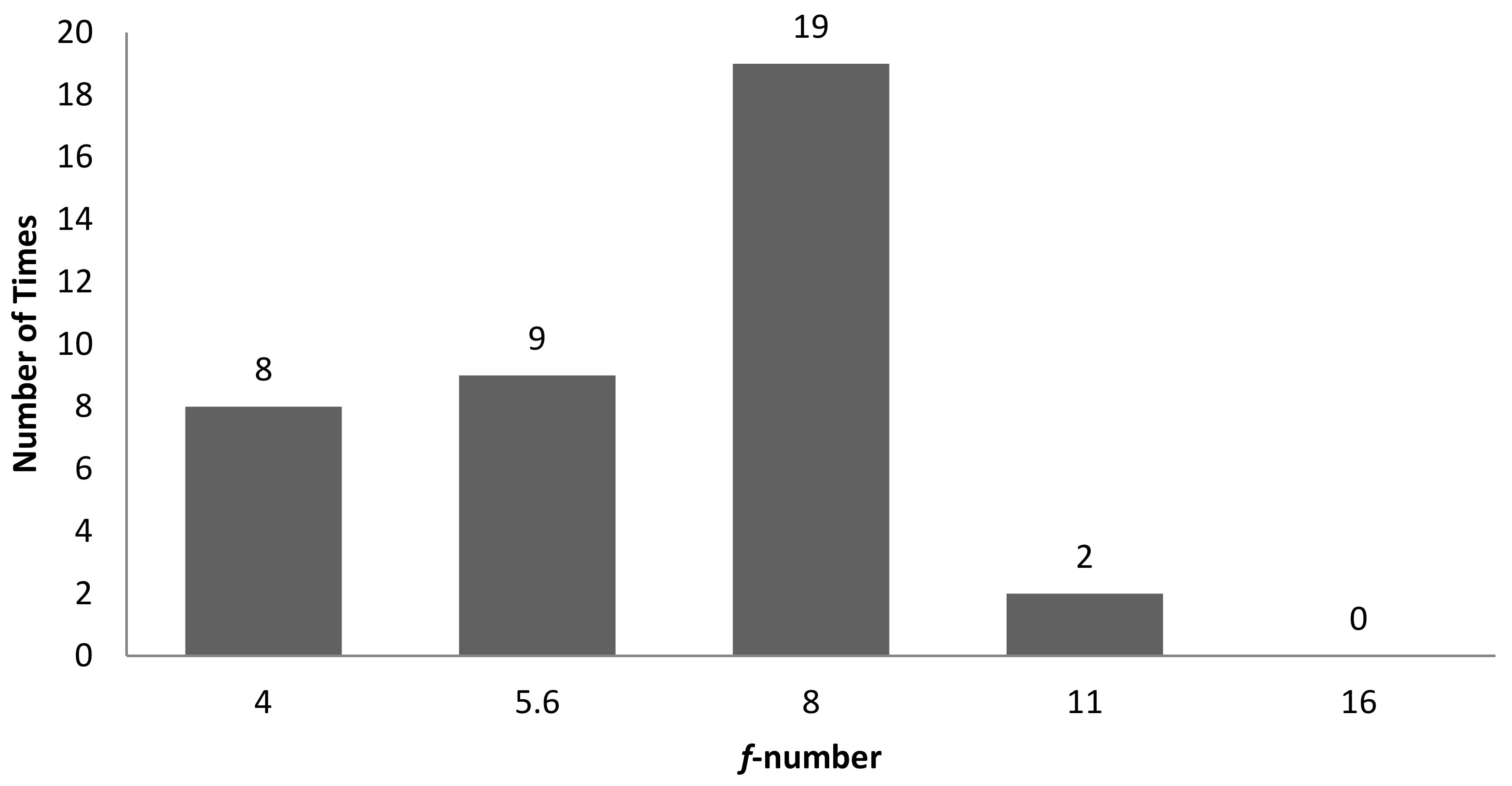
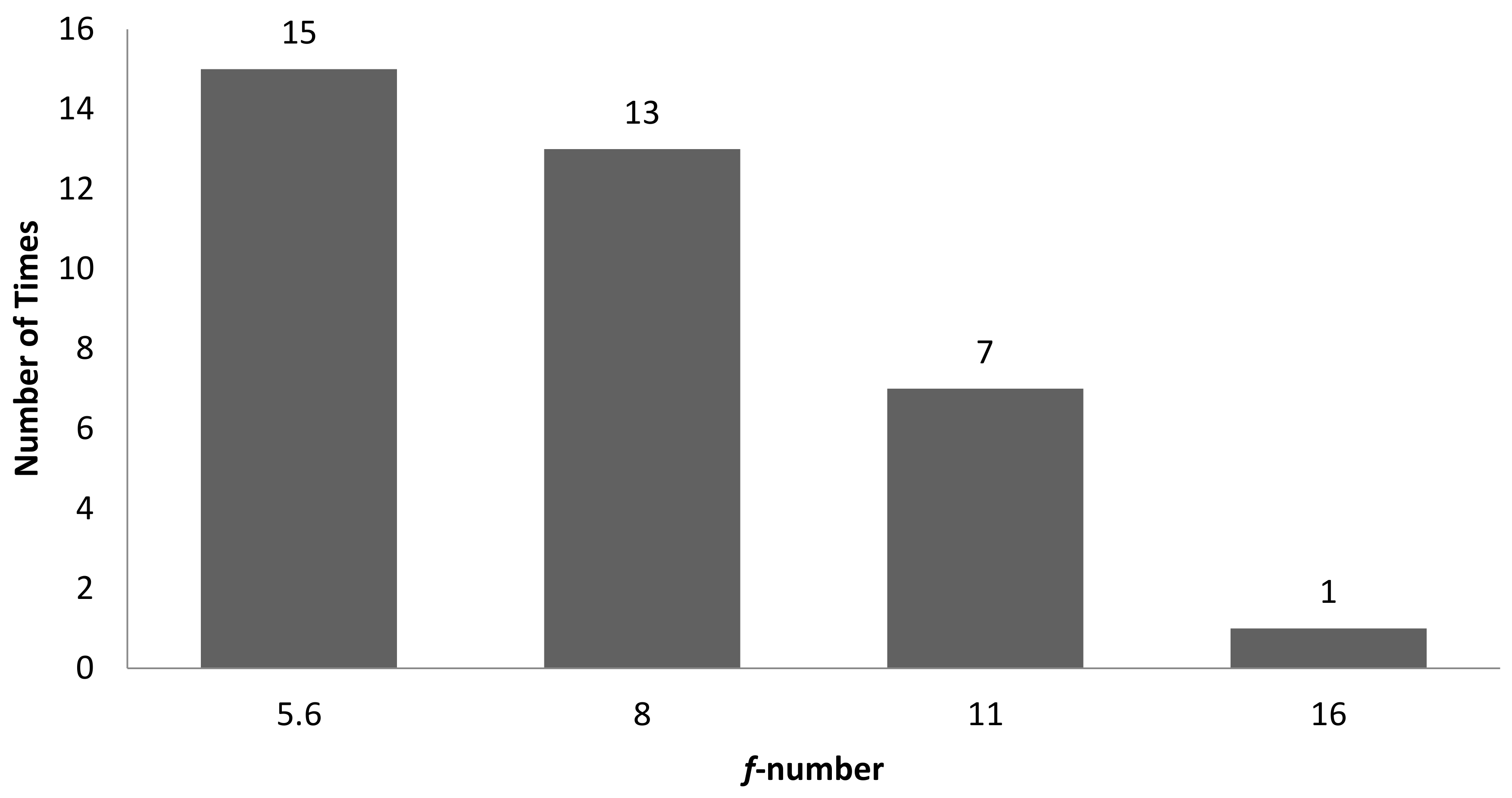
| S. No. | Correlation | R2 | Camera Setting |
|---|---|---|---|
| 1 | Correlation (GLCM) vs. Sa | 0.7354 | f-number 8, shutter speed 1/200 s |
| 2 | Correlation (GLCM) vs. Sq | 0.7438 |
| S. No. | Correlation | R2 | Camera Setting |
|---|---|---|---|
| 1 | Entropy (GLCM) vs. Sa | 0.8208 | f-number 8, shutter speed 1/50 s |
| 2 | Entropy (GLCM) vs. Sq | 0.7352 | |
| 3 | Energy vs. Sp | 0.7347 | f-number 16, shutter speed 1/100 s |
| 4 | Energy (GLCM) vs. Sp | 0.7202 | |
| 5 | Energy vs. Sz | 0.7015 | |
| 6 | Entropy vs. Sz | 0.7354 | |
| 7 | Entropy (GLCM) vs. Sz | 0.7565 | |
| 8 | Homogeneity (GLCM) vs. Sz | 0.7704 | |
| 9 | Energy vs. S10z | 0.8916 | |
| 10 | Energy (GLCM) vs. S10z | 0.8955 | |
| 11 | W/B vs. Sdq | 0.8151 | f-number 22, shutter speed 1/100 s |
| 12 | W/B vs. Sdr | 0.8294 | |
| 13 | Contrast (GLCM) vs. Sa | 0.749 | f-number 22, shutter speed 1/200 s |
| 14 | Correlation (GLCM) vs. Sa | 0.806 | |
| 15 | Contrast (GLCM) vs. Sq | 0.7358 | |
| 16 | Correlation (GLCM) vs. Sq | 0.8148 | |
| 17 | Contrast (GLCM) vs. Sp | 0.7368 | |
| 18 | Correlation (GLCM) vs. Sp | 0.8403 | |
| 19 | Correlation (GLCM) vs. S10z | 0.7316 |
Publisher’s Note: MDPI stays neutral with regard to jurisdictional claims in published maps and institutional affiliations. |
© 2022 by the authors. Licensee MDPI, Basel, Switzerland. This article is an open access article distributed under the terms and conditions of the Creative Commons Attribution (CC BY) license (https://creativecommons.org/licenses/by/4.0/).
Share and Cite
Jayabarathi, S.B.; Ratnam, M.M. Comparison of Correlation between 3D Surface Roughness and Laser Speckle Pattern for Experimental Setup Using He-Ne as Laser Source and Laser Pointer as Laser Source. Sensors 2022, 22, 6003. https://doi.org/10.3390/s22166003
Jayabarathi SB, Ratnam MM. Comparison of Correlation between 3D Surface Roughness and Laser Speckle Pattern for Experimental Setup Using He-Ne as Laser Source and Laser Pointer as Laser Source. Sensors. 2022; 22(16):6003. https://doi.org/10.3390/s22166003
Chicago/Turabian StyleJayabarathi, Suganandha Bharathi, and Mani Maran Ratnam. 2022. "Comparison of Correlation between 3D Surface Roughness and Laser Speckle Pattern for Experimental Setup Using He-Ne as Laser Source and Laser Pointer as Laser Source" Sensors 22, no. 16: 6003. https://doi.org/10.3390/s22166003