
Correlation Study of 3D Surface Roughness of Milled Surfaces with Laser Speckle Pattern


Abstract
:1. Introduction
- Use of inexpensive laser pointers for producing the laser speckle pattern.
- A correlation study of the characteristic features extracted from the image of the laser speckle pattern of the milled surface and 3D surface roughness parameters, measured with commercial 3D metrology system.
- A study about the influence of the angle of illumination of a laser beam, f-number and the shutter speed of a camera setting on the correlation of 3D surface roughness parameters with the characteristic features extracted from the laser pattern image of the milled surface.
2. Materials and Methods
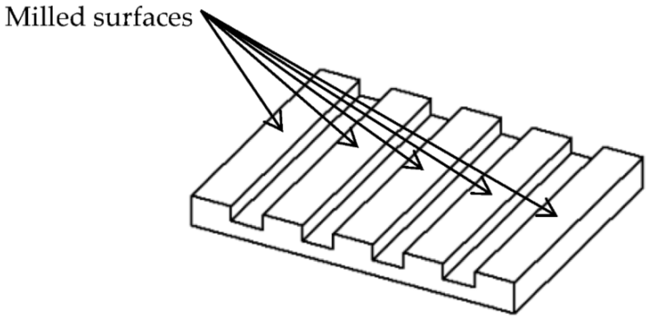
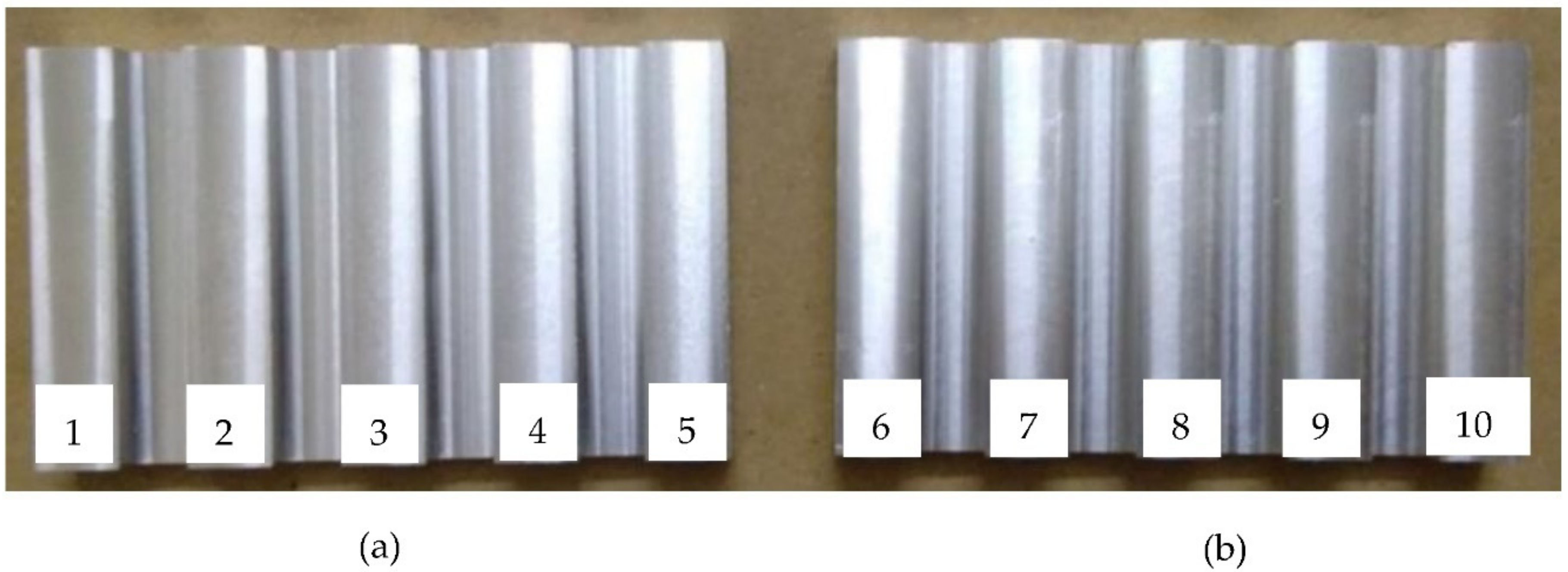
2.1. Sample Preparation
- Arithmetic Mean Height (Sa)
- Root-Mean-Square Height (Sq)
- Maximum Peak Height (Sp)
- Maximum Valley Depth (Sv)
- Maximum Height (Sz)
- Ten Point Height (S10z)
- Skewness (Ssk)
- Kurtosis (Sku)
- Root Mean Square Gradient (Sdq)
- Developed Interfacial area ratio (Sdr)
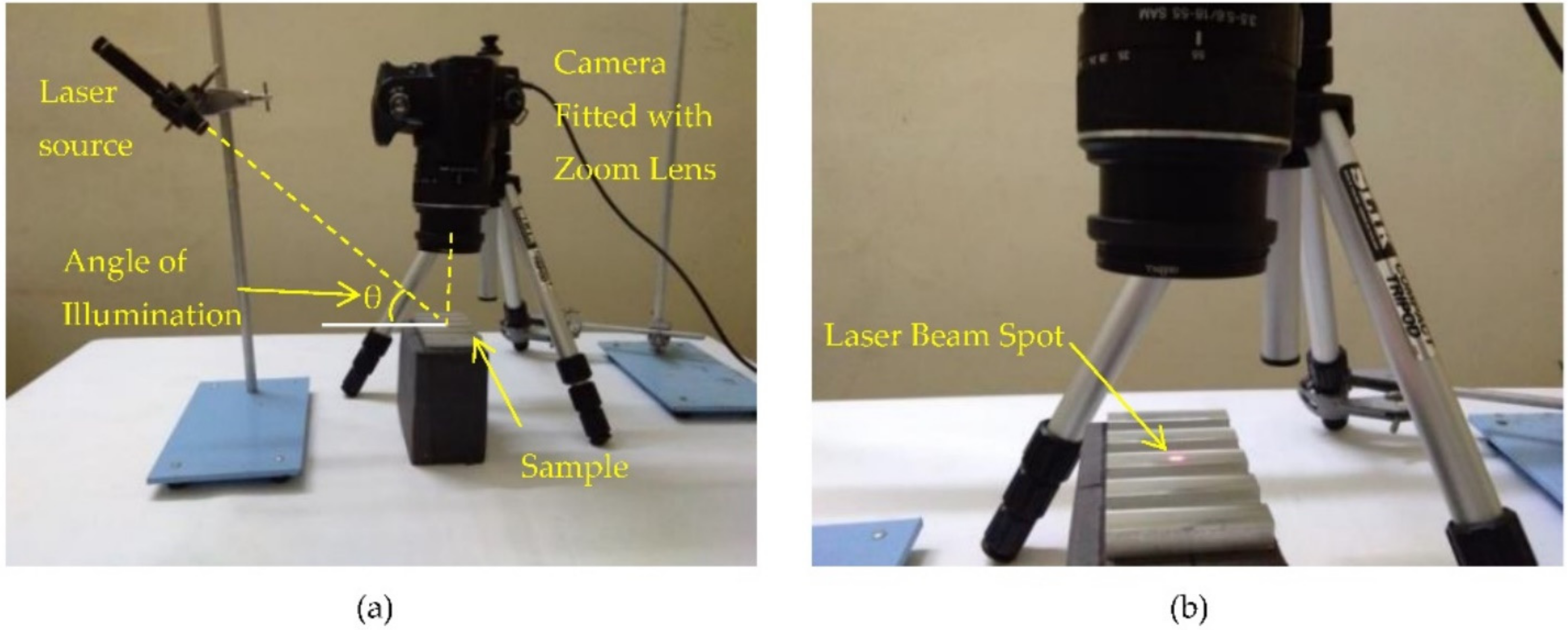
2.2. Experimental Setup
2.3. Characteristic Features Extraction
- Histogram-based (statistical) features
- ∘
- MeanMean of gray value of the image m obtained from the original image f(x,y) of size M × N given by Equation (1).where f(x,y) is the gray value of pixel at coordinates (x,y)
- ∘
- Standard deviationStandard deviation σ of an image is given by Equation (2).where:rj is the jth gray level.L is the total possible gray level value.p(rj) is the probability of occurrences of rj.m is the mean of gray values of the image.
- ∘
- EnergyThe energy descriptor, which is also known as uniformity, measures how pixel values are distributed along the gray level range and can be calculated for grayscale images using Equation (3).where:rj is the jth gray level.L is total possible gray level value.p(rj) is the probability of occurrences of rj.
- ∘
- EntropyThe entropy descriptor provides information about the complexity of the image, as given by Equation (4).where:rj is the jth gray level.L is total possible gray level value.p(rj) is the probability of occurrences of rj.
- Texture features
- ∘
- Normalised descriptor of roughness RNormalised descriptor of roughness R is as given in Equation (5).where:σ2 is variance.L is total possible gray level value
- Gray level co-occurrence matrix (GLCM)The histogram-based texture descriptors do not provide any information about the spatial relationship among pixels. This information can be obtained using the gray level co-occurrence matrix (GLCM). The matrix holds the information about the number of times pixels with intensities ri and rj occur in the image f(x,y) in the position specified by the displacement vector d = (dx,dy) and orientation θ. In this work, the default values of the displacement vector and orientation, as in the MATLAB software, that is d = (0,1) and orientation of 0°, were used. The matrix is normalized as given in Equation (6).where:Ng(i,j) is the normalized gray level co-occurrence matrix.g(i,j) is the element of the gray level co-occurrence matrix.The following texture-based features are computed using a normalized GLCM, Ng(i,j).
- ∘
- Maximum Probability as given by Equation (7).
- ∘
- Correlation as given by Equation (8).where:µi is the mean of the row sums of Ng(i,j).µj is the mean of column sums of Ng(i,j).σi is the standard deviation of row sums of Ng(i,j).σj is the standard deviation of column sums of Ng(i,j).
- ∘
- Contrast as given by Equation (9).
- ∘
- Energy as given by Equation (10).
- ∘
- Homogeneity as given by Equation (11).
- ∘
- Entropy as given by Equation (12).
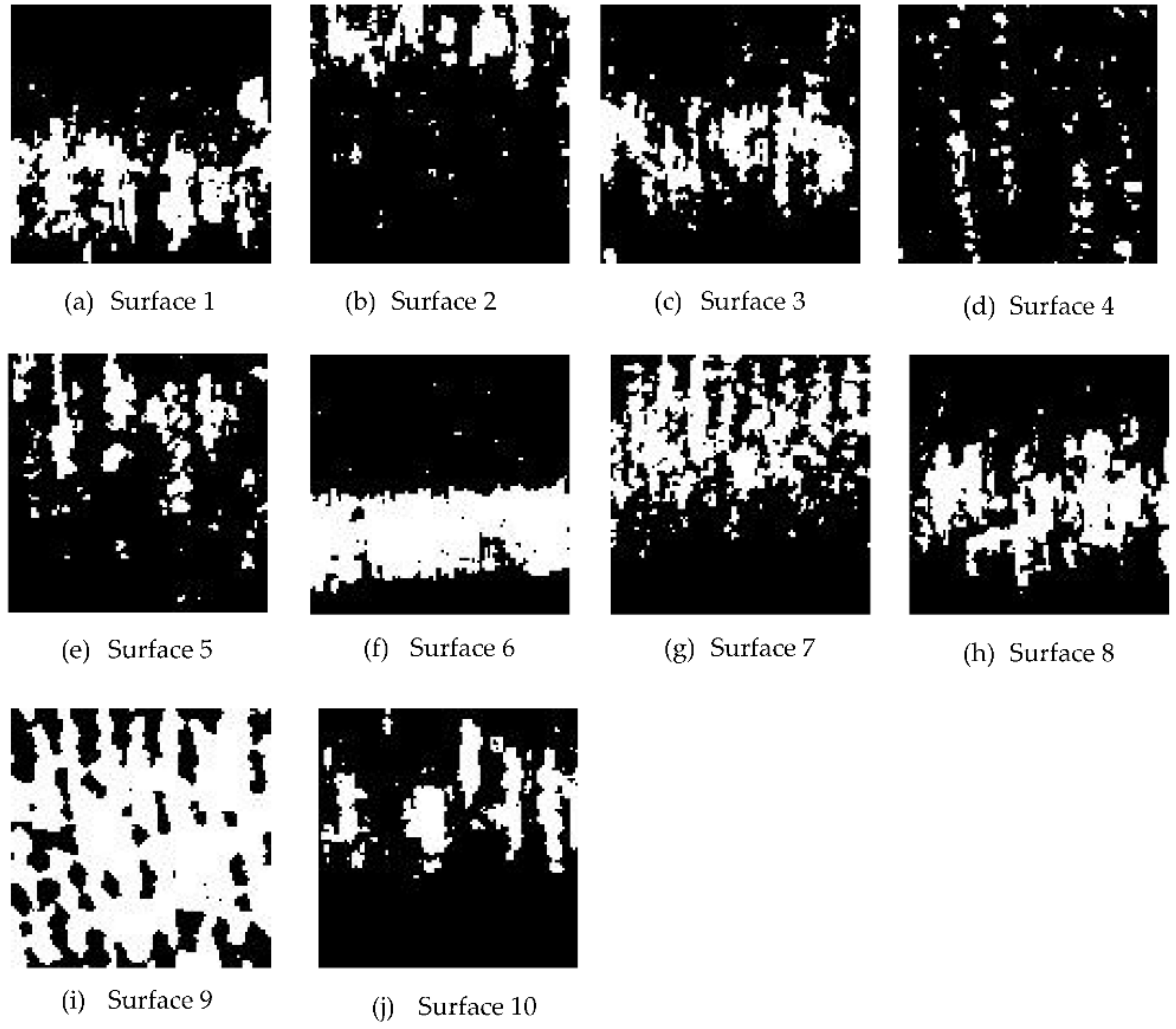
- From the binary image, the following characteristic features were extracted:
- ∘
- Total white pixels to total black pixels ratio (W/B)
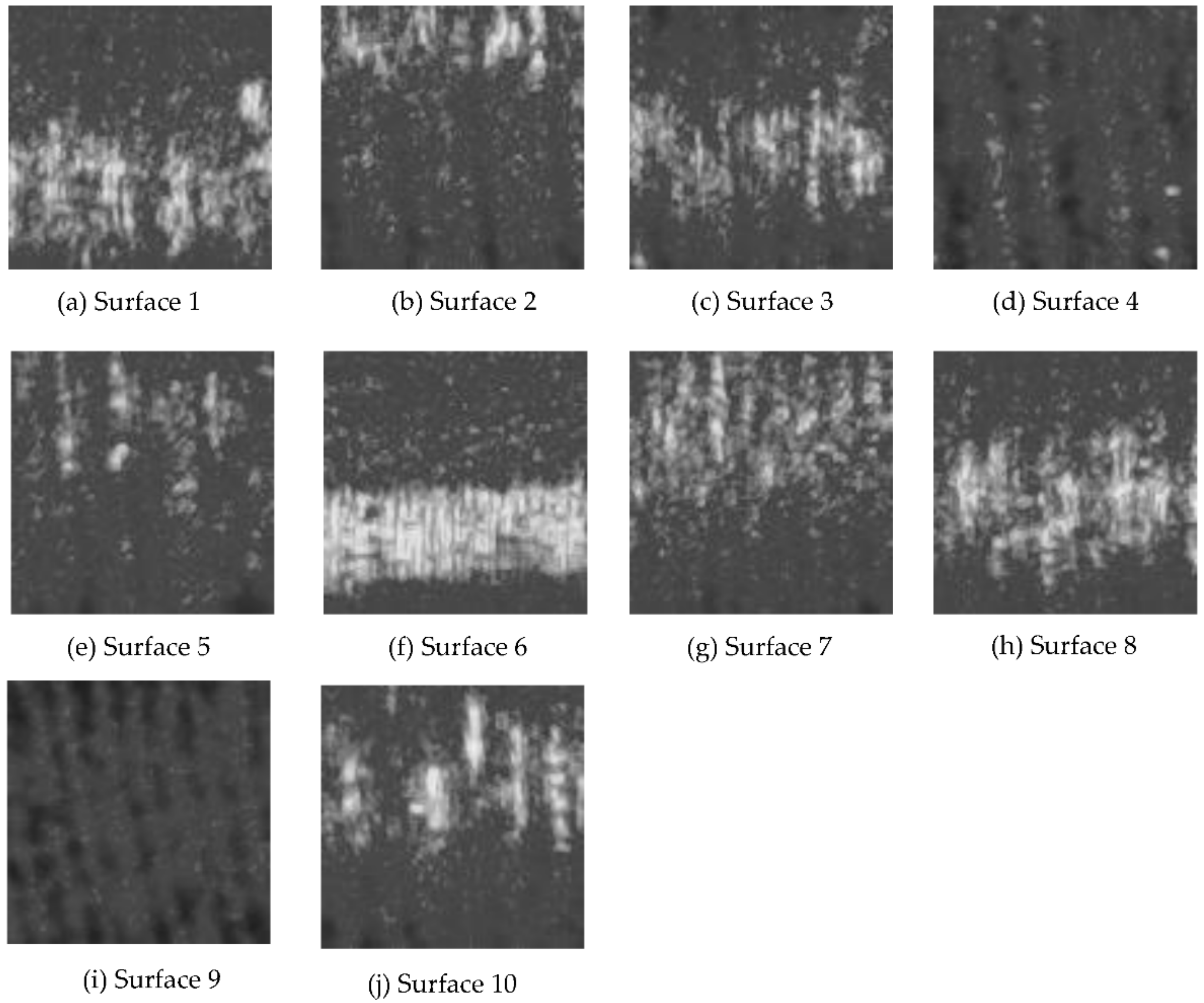
3. Results and Discussion
4. Conclusions
- An inexpensive laser pointer can be used for producing a laser speckle pattern.
- Good correlations between the characteristic features and 3D surface roughness were obtained.
- It was found that the angle of illumination, f-number and shutter speed combination affect the coefficient of determinations.
5. Recommendation for Future Work
- In this work, the authors limited their study using GLCM to displacement d = 1 and orientation . Future correlation studies should be carried out using GLCM for different combinations of displacement and orientation.
- A study should also be conducted on how the wavelength of a laser and the distance of the camera from the sample affect the correlation.
Author Contributions
Funding
Institutional Review Board Statement
Data Availability Statement
Acknowledgments
Conflicts of Interest
References
- Degarmo, E.P.; Black, J.T.; Kohser, R.A. Materials and Processess in Manufacturing, 8th ed.; Prentice-Hall International: Upper Saddle River, NJ, USA, 1997; p. 288. [Google Scholar]
- Liu, J.; Lu, E.; Yi, H.; Wang, M.; Ao, P. A new surface roughness measurement method based on a color distribution statistical matrix. Measurement 2017, 103, 165–178. [Google Scholar] [CrossRef]
- Rifai, A.P.; Aoyama, H.; Tho, N.H.; Md Dawal, S.Z.; Masruroh, N.A. Evaluation of turned and milled surfaces roughness using convolutional neural network. Measurement 2020, 161, 107860. [Google Scholar] [CrossRef]
- Agrawal, A.; Goel, S.; Rashid, W.B.; Price, M. Prediction of surface roughness during hard turning of AISI 4340 steel (69 HRC). Appl. Soft Comput. 2015, 30, 279–286. [Google Scholar] [CrossRef] [Green Version]
- Manojlovic, L.M.; Zivanov, M.B.; Marincic, A.S. White-Light Interferometric Sensor for Rough Surface Height Distribution Measurement. IEEE Sens. J. 2010, 10, 1125–1132. [Google Scholar] [CrossRef]
- Petzold, S.; Klett, J.; Schauer, A.; Osswald, T.A. Surface roughness of polyamide 12 parts manufactured using selective laser sintering. Polym. Test. 2019, 80, 106094. [Google Scholar] [CrossRef]
- Tsigarida, A.; Tsampali, E.; Konstantinidis, A.A.; Stefanidou, M. On the use of confocal microscopy for calculating the surface microroughness and the respective hydrophobic properties of marble specimens. J. Build. Eng. 2021, 33, 101876. [Google Scholar] [CrossRef]
- Goh, C.S.; Ratnam, M.M. Assessment of Areal (Three-Dimensional) Roughness Parameters of Milled Surface Using Charge-Coupled Device Flatbed Scanner and Image Processing. Exp. Tech. 2016, 40, 1099–1107. [Google Scholar] [CrossRef]
- Xu, D.; Yang, Q.; Dong, F.; Krishnaswamy, S. Evaluation of surface roughness of a machined metal surface based on laser speckle pattern. J. Eng. 2018, 2018, 773–778. [Google Scholar] [CrossRef]
- Mahashar Ali, J.; Siddhi Jailani, H.; Murugan, M. Surface roughness evaluation of electrical discharge machined surfaces using wavelet transform of speckle line images. Measurement 2020, 149, 107029. [Google Scholar] [CrossRef]
- Soares, H.C.; Meireles, J.B.; Castro, A.O.; Huguenin, J.A.O.; Schmidt, A.G.M.; Da Silva, L. Tsallis threshold analysis of digital speckle patterns generated by rough surfaces. Phys. A Stat. Mech. Appl. 2015, 432, 1–8. [Google Scholar] [CrossRef]
- Joshi, K.; Patil, B. Prediction of Surface Roughness by Machine Vision using Principal Components based Regression Analysis. Procedia Comput. Sci. 2020, 167, 382–391. [Google Scholar] [CrossRef]
- Dias, M.R.B.; Dornelas, D.; Balthazar, W.F.; Huguenin, J.A.O.; Da Silva, L. Lacunarity study of speckle patterns produced by rough surfaces. Phys. A Stat. Mech. Appl. 2017, 486, 328–336. [Google Scholar] [CrossRef]
- Baradit, E.; Gatica, C.; Yáñez, M.; Figueroa, J.C.; Guzmán, R.; Catalán, C. Surface roughness estimation of wood boards using speckle interferometry. Opt. Lasers Eng. 2020, 128, 106009. [Google Scholar] [CrossRef]
- Goch, G.; Peters, J.; Lehmann, P.; Liu, H. Requirements for the Application of Speckle Correlation Techniques to On-Line Inspection of Surface Roughness. CIRP Ann. 1999, 48, 467–470. [Google Scholar] [CrossRef]
- Dhanasekar, B.; Mohan, N.K.; Bhaduri, B.; Ramamoorthy, B. Evaluation of surface roughness based on monochromatic speckle correlation using image processing. Precis. Eng. 2008, 32, 196–206. [Google Scholar] [CrossRef]
- Toh, S.L.; Shang, H.M.; Tay, C.J. Surface-roughness study using laser speckle method. Opt. Lasers Eng. 1998, 29, 217–225. [Google Scholar] [CrossRef]
- Tchvialeva, L.; Markhvida, I.; Zeng, H.; McLean, D.I.; Lui, H.; Lee, T.K. Surface roughness measurement by speckle contrast under the illumination of light with arbitrary spectral profile. Opt. Lasers Eng. 2010, 48, 774–778. [Google Scholar] [CrossRef]
- Leonard, L.C.; Toal, V. Roughness measurement of metallic surfaces based on the laser speckle contrast method. Opt. Lasers Eng. 1998, 30, 433–440. [Google Scholar] [CrossRef]
- Smith, G.T. Industrial Metrology: Surfaces and Roundness; Springer: London, UK, 2002. [Google Scholar]
- Wang, T.; Xie, L.-J.; Wang, X.-B.; Shang, T.-Y. 2D and 3D milled surface roughness of high volume fraction SiCp/Al composites. Def. Technol. 2015, 11, 104–109. [Google Scholar] [CrossRef] [Green Version]
- Molnár, V. Minimization Method for 3D Surface Roughness Evaluation Area. Machines 2021, 9, 192. [Google Scholar] [CrossRef]
- Zhang, X.; Zheng, Y.; Suresh, V.; Wang, S.; Li, Q.; Li, B.; Qin, H. Correlation approach for quality assurance of additive manufactured parts based on optical metrology. J. Manuf. Processes 2020, 53, 310–317. [Google Scholar] [CrossRef]
- Fuji, H.; Asakura, T.; Shindo, Y. Measurement of surface roughness properties by means of laser speckle techniques. Opt. Commun. 1976, 16, 68–72. [Google Scholar] [CrossRef]
- Zheng, Q.; Mashiwa, N.; Furushima, T. Evaluation of large plastic deformation for metals by a non-contacting technique using digital image correlation with laser speckles. Mater. Des. 2020, 191, 108626. [Google Scholar] [CrossRef]
- ISO 25178-2:2012. Geometrical Product Specifications(GPS)—Surface Texture: Areal—Part 2: Terms, Definitions and Surface Texture Parameters; International Organization for Standardization, Vernier: Geneva, Switzerland, 2012. [Google Scholar]
- Ravimal, D.; Kim, H.; Koh, D.; Hong, J.H.; Lee, S.-K. Image-Based Inspection Technique of a Machined Metal Surface for an Unmanned Lapping Process. Int. J. Precis. Eng. Manuf.-Green Technol. 2020, 7, 547–557. [Google Scholar] [CrossRef] [Green Version]
- Marques, O. Practical Image and Video Processing using MATLAB; John Wiley & Sons: Hoboken, NJ, USA, 2011. [Google Scholar]
- Xiaomei, X. Non-contact surface roughness measurement based on laser technology and neural network. In Proceedings of the 2009 International Conference on Mechatronics and Automation, Changchun, China, 9–12 August 2009; pp. 4474–4478. [Google Scholar]


| Surface No. | Spindle Speed (rpm) | Feed Rate (mm/min) | Depth of Cut (mm) | Sa (µm) | Sq (µm) | Sp (µm) | Sv (µm) | Sz (µm) | S10z (µm) | Ssk | Sku | Sdq | Sdr (%) |
|---|---|---|---|---|---|---|---|---|---|---|---|---|---|
| 1 | 1000 | 120 | 1 | 0.931 | 1.117 | 4.070 | 3.889 | 7.959 | 6.187 | −0.044 | 2.415 | 0.161 | 1.305 |
| 2 | 1000 | 280 | 1 | 1.046 | 1.322 | 8.081 | 7.774 | 15.855 | 9.217 | 0.281 | 3.398 | 0.177 | 1.553 |
| 3 | 1000 | 440 | 1 | 1.325 | 1.675 | 9.809 | 6.795 | 16.605 | 10.826 | 0.146 | 3.442 | 0.191 | 1.790 |
| 4 | 1000 | 600 | 1 | 1.162 | 1.567 | 11.639 | 13.136 | 24.775 | 14.423 | 0.275 | 6.054 | 0.242 | 2.636 |
| 5 | 1000 | 760 | 1 | 1.254 | 1.816 | 10.948 | 8.678 | 19.626 | 16.608 | 0.360 | 6.142 | 0.318 | 4.565 |
| 6 | 2500 | 120 | 1 | 0.748 | 0.902 | 5.681 | 6.960 | 12.641 | 5.122 | 0.335 | 2.473 | 0.185 | 1.722 |
| 7 | 2500 | 280 | 1 | 0.968 | 1.156 | 5.437 | 8.607 | 14.045 | 6.387 | −0.177 | 6.528 | 0.185 | 1.749 |
| 8 | 2500 | 440 | 1 | 0.974 | 1.225 | 7.169 | 6.327 | 13.496 | 7.440 | −0.124 | 4.374 | 0.196 | 1.830 |
| 9 | 2500 | 600 | 1 | 1.058 | 1.326 | 8.617 | 9.490 | 18.106 | 8.325 | 0.000 | 3.152 | 0.192 | 1.888 |
| 10 | 2500 | 760 | 1 | 1.113 | 1.417 | 9.640 | 6.377 | 16.016 | 10.246 | 0.257 | 3.715 | 0.193 | 1.811 |
| Correlation | R2 | Camera Setting |
|---|---|---|
| Correlation (GLCM) vs. Sa | 0.7354 | f-number 8 shutter speed 1/200 s |
| Correlation (GLCM) vs. Sq | 0.7438 |
| Correlation | R2 | Camera Setting |
|---|---|---|
| Entropy (GLCM) vs. Sa | 0.8208 | f-number 8 shutter speed 1/50 s |
| Entropy (GLCM) vs. Sq | 0.7352 | |
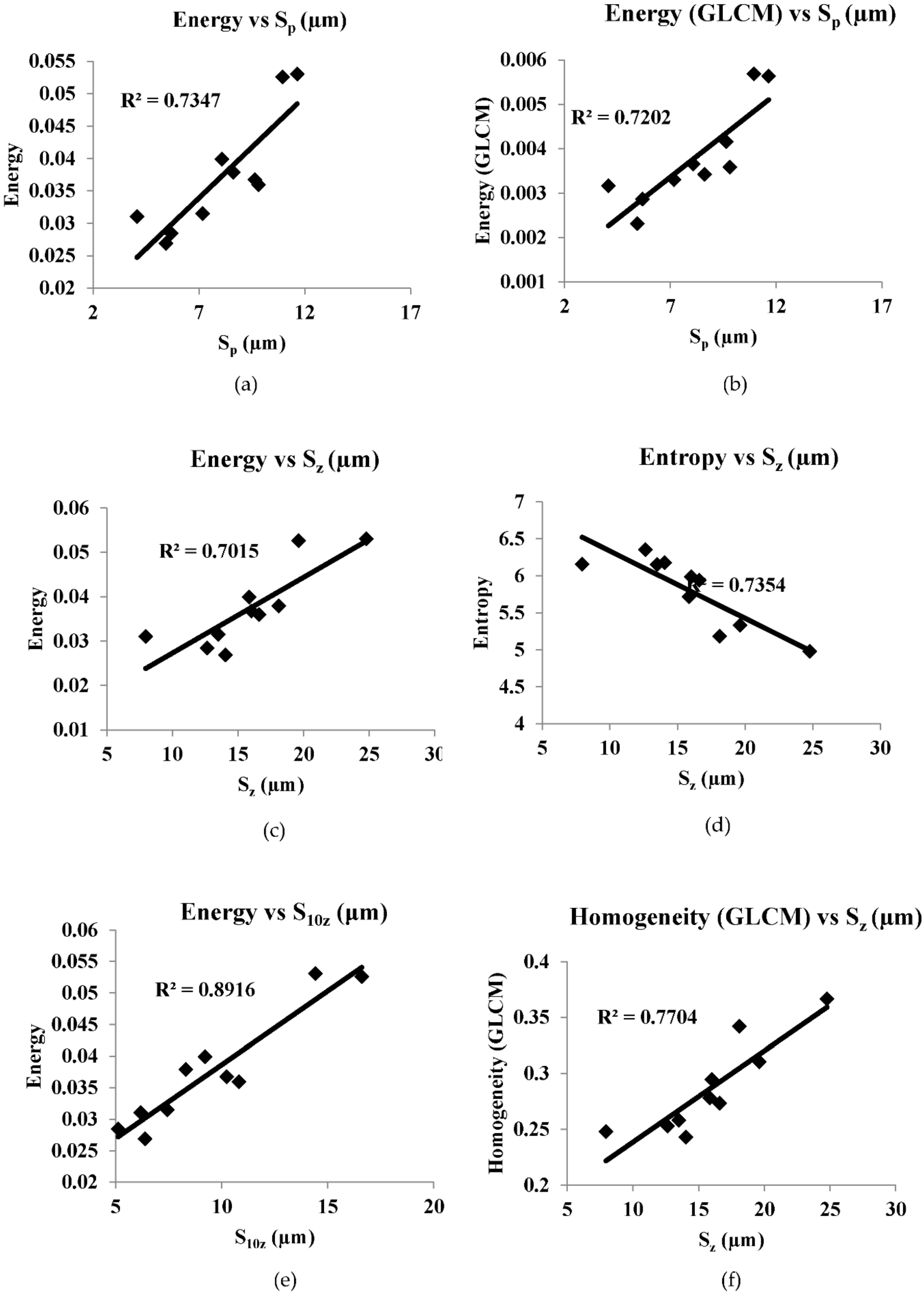
| Energy vs. Sp | 0.7347 | f-number 16 shutter speed 1/100 s |
| Energy (GLCM) vs. Sp | 0.7202 | |
| Energy vs. Sz | 0.7015 | |
| Entropy vs. Sz | 0.7354 | |
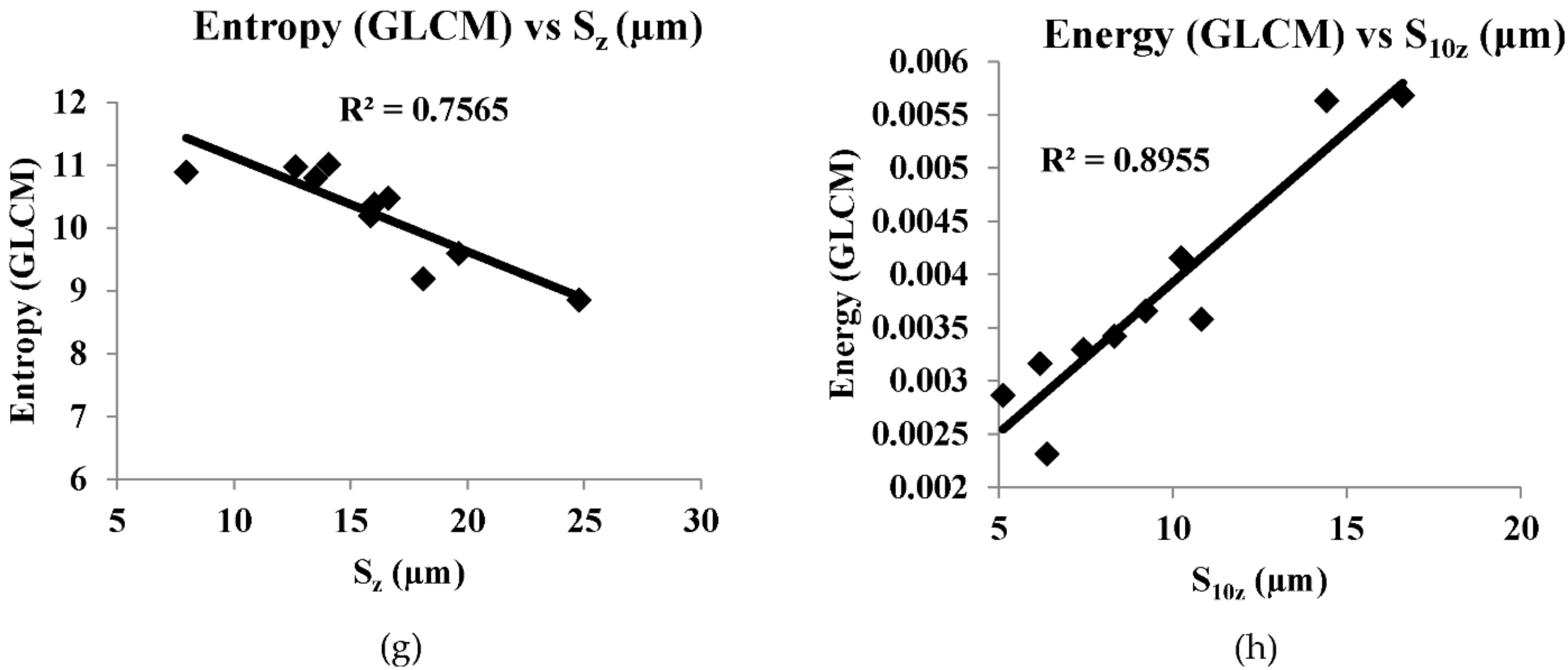
| Entropy (GLCM) vs. Sz | 0.7565 | |
| Homogeneity (GLCM) vs. Sz | 0.7704 | |
| Energy vs. S10z | 0.8916 | |
| Energy (GLCM) vs. S10z | 0.8955 | |
| W/B vs. Sdq | 0.8151 | f-number 22 shutter speed 1/100 s |
| W/B vs. Sdr | 0.8294 | |
| Contrast (GLCM) vs. Sa | 0.749 | f-number 22 shutter speed 1/200 s |
| Correlation (GLCM) vs. Sa | 0.806 | |
| Contrast (GLCM) vs. Sq | 0.7358 | |
| Correlation (GLCM) vs. Sq | 0.8148 | |
| Contrast (GLCM) vs. Sp | 0.7368 | |
| Correlation (GLCM) vs. Sp | 0.8403 | |
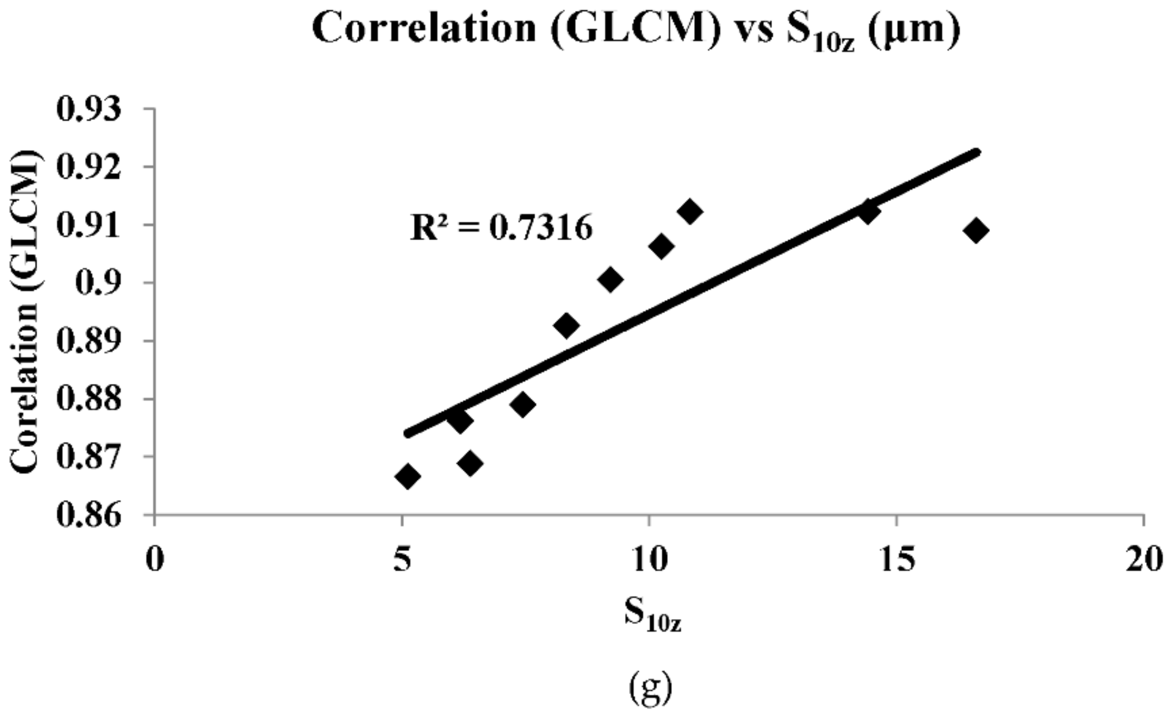
| Correlation (GLCM) vs. S10z | 0.7316 |
Publisher’s Note: MDPI stays neutral with regard to jurisdictional claims in published maps and institutional affiliations. |
© 2022 by the authors. Licensee MDPI, Basel, Switzerland. This article is an open access article distributed under the terms and conditions of the Creative Commons Attribution (CC BY) license (https://creativecommons.org/licenses/by/4.0/).
Share and Cite
Jayabarathi, S.B.; Ratnam, M.M. Correlation Study of 3D Surface Roughness of Milled Surfaces with Laser Speckle Pattern. Sensors 2022, 22, 2842. https://doi.org/10.3390/s22082842
Jayabarathi SB, Ratnam MM. Correlation Study of 3D Surface Roughness of Milled Surfaces with Laser Speckle Pattern. Sensors. 2022; 22(8):2842. https://doi.org/10.3390/s22082842
Chicago/Turabian StyleJayabarathi, Suganandha Bharathi, and Mani Maran Ratnam. 2022. "Correlation Study of 3D Surface Roughness of Milled Surfaces with Laser Speckle Pattern" Sensors 22, no. 8: 2842. https://doi.org/10.3390/s22082842