
A Simplified Algorithm for Setting the Observer Parameters for Second-Order Systems with Persistent Disturbances Using a Robust Observer


Abstract
:1. Introduction
- Ci. The width of the convergence region of the observer error for the unknown state is expressed in terms of the interaction between the observer parameters and the disturbance in terms of the observer error dynamics. Thus, the desired estimation accuracy can be defined by the user by setting the observer parameters in accordance with this relationship. In contrast:
- −
- In [21], the dependence of the width of the convergence region on the observer parameters and disturbance terms is not determined.
- −
- In [10], the width of the convergence region is expressed in terms of the bounds of the disturbances and measurement noise, but bounded disturbances are not considered in the dynamics of the estimation error of the known state, so the effect of these disturbances is not considered in the convergence region.
- −
- In [23], the width of the convergence region is expressed in terms of the bounds of the disturbances of the dynamics of the estimation error of the known state, but the effect of observer parameters and bounded disturbance of the dynamics of the estimation error of the unknown state are not considered.
- Cii. The properties and limits of this width are determined. It was found that this width has a minimum point and a vertical asymptote with respect to one of the observer parameters, and their coordinates were determined. Then, the highest accuracy of the state estimation can be obtained by setting the observer parameters equal or similar to the coordinates of the minimum. In contrast, in [21,23,25]: (i) the properties, limits, and minimum of the width of the convergence region of the estimation error for the unknown state are not determined; (ii) the observer parameter values that lead to the lowest width of the convergence region are not determined.
- Ciii. The algorithm considers the combined effect of disturbance terms and observer parameters on the width of the convergence region.
- (i)
- Advantage A1. It involves a significantly simpler definition of observer parameters: the fulfillment of Riccati equation conditions, solution of LMI constraints, and fulfillment of eigenvalue conditions are not required, thus, reducing the trial-and-error effort. In contrast, the fulfillment of these conditions is commonly required in closely related observer strategies, for instance [10,23,26].
- (ii)
- (iii)
- (iv)
2. Bioreactor Model
3. Preliminaries: Observer and Bounds for the Transient and Steady Behavior of the Observer Error
3.1. Observer
3.2. Mathematical Definitions
3.3. Convergence of the Observer Error for the Known State
3.4. Bounds for the Transient and Steady Behavior of the Observer Error for the Unknown State
4. Formulation of the Algorithm for Setting the Observer Parameters and Determination of the Width of the Convergence Region of the Observer Error in Terms of the Observer Parameters
4.1. Determination of the Width of the Convergence Region of the Observer Error
4.2. Formulation of the Algorithm for Setting the Observer Parameters
| Algorithm 1: Algorithm for setting the parameters of the observer (3)–(5). | |
| Step | Description |
| 1 | Cast the system model in the form (1)–(2) and identify the known state , the unknown state , and the terms , ,, , . |
| 2 | Obtain the values of that satisfy Assumption 2 and the values of , , satisfying Equation (18). To this end, the values of , can be obtained by the simulation of ,, based on the , model, with model parameter values obtained from either closely related studies or offline fitting. |
| 3 | Set the values of , to define:
where and the minimum point of is given by Equation (22): ; |
| 4 | Set a high value of to define the update rate of , according to Equation (5). Set a high value of to define the convergence rate of , according to Equation (11). |
- −
- −
- Anaerobic bioreactor for hydrogen production via the dark fermentation of glucose: estimation of influent glucose concentration based on known reactor glucose con-centration—see [3].
- −
- Fed-batch bioreactor for ethanol production: (i) estimation of the rate of enzymatic hydrolysis based on known substrate (starch) concentration; (ii) estimation of the glucose consumption rate based on known glucose concentration—see [4].
- −
- Membrane fuel cell: estimation of stack temperature based on known oxygen pres-sure—see [34].
- −
- Photovoltaic system: estimation of the power gradient based on known generated electric power—see [35].
- −
- DC-DC buck converter: estimation of the time derivative of the output tracking er-ror based on the known average output voltage—see [36].
- −
- Second-order underactuated mechanical system: estimation of the time derivative of the pole angle—see [20].
- (a)
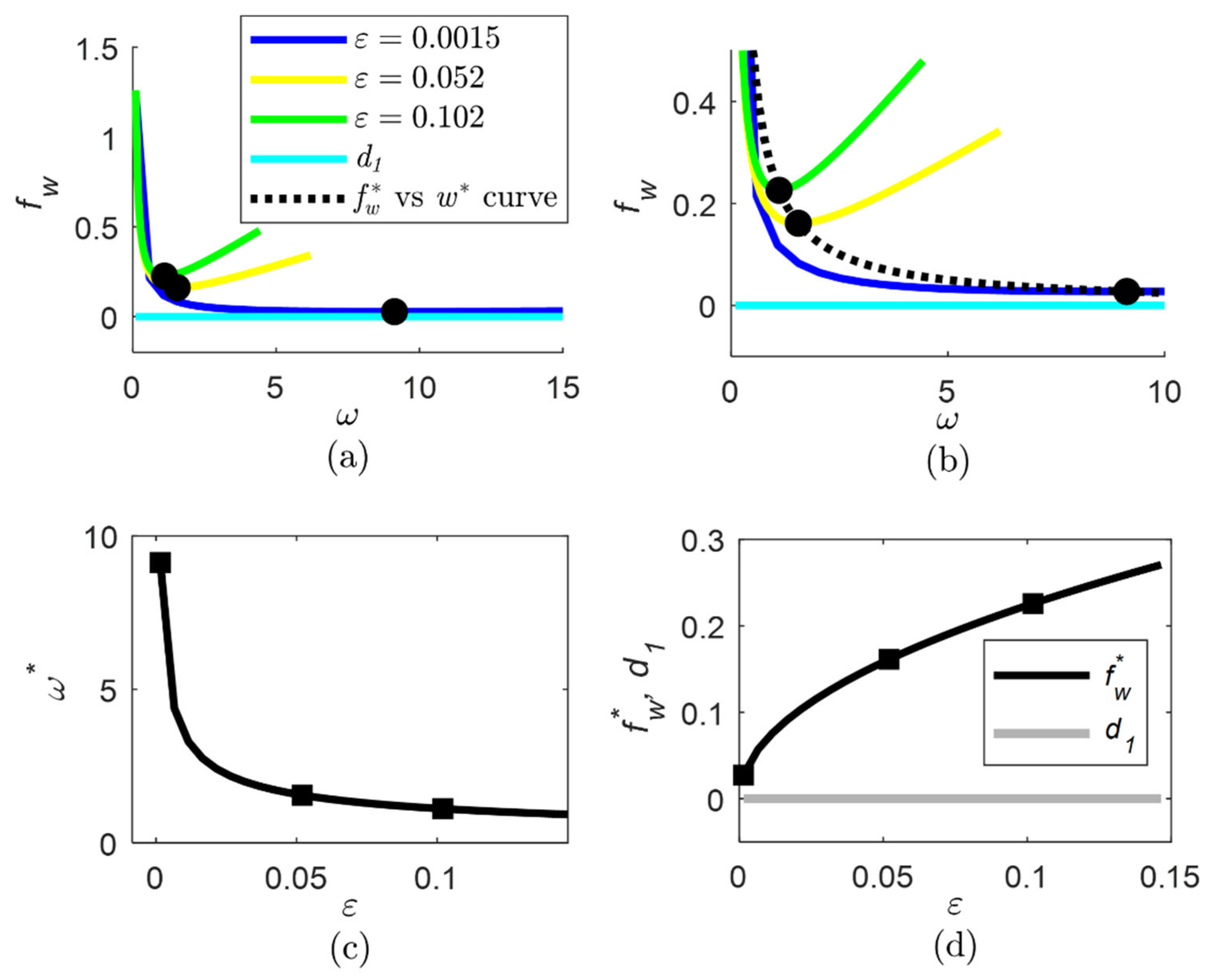
- The convergence region is expressed as a function of the combined effect of observer parameters and disturbance terms—see Equations (19) and (20). Then, the desired estimation accuracy can be defined by the user by properly setting the observer parameters in accordance with this relationship.
- (b)
- The properties of this expression are determined in terms of the observer parameters, including the limits and the coordinates of the minimum—see Equations (21)–(23). In turn, these properties allow choosing ω, ε values to avoid an undesired overlarge f_w value, and the lowest f_w value is obtained by using the coordinates of the minimum, that is, ω=ω^*, according to Equation (22). Thus, the highest accuracy of the state estimation is obtained by setting the observer parameters equal or similar to the coordinates of the minimum.
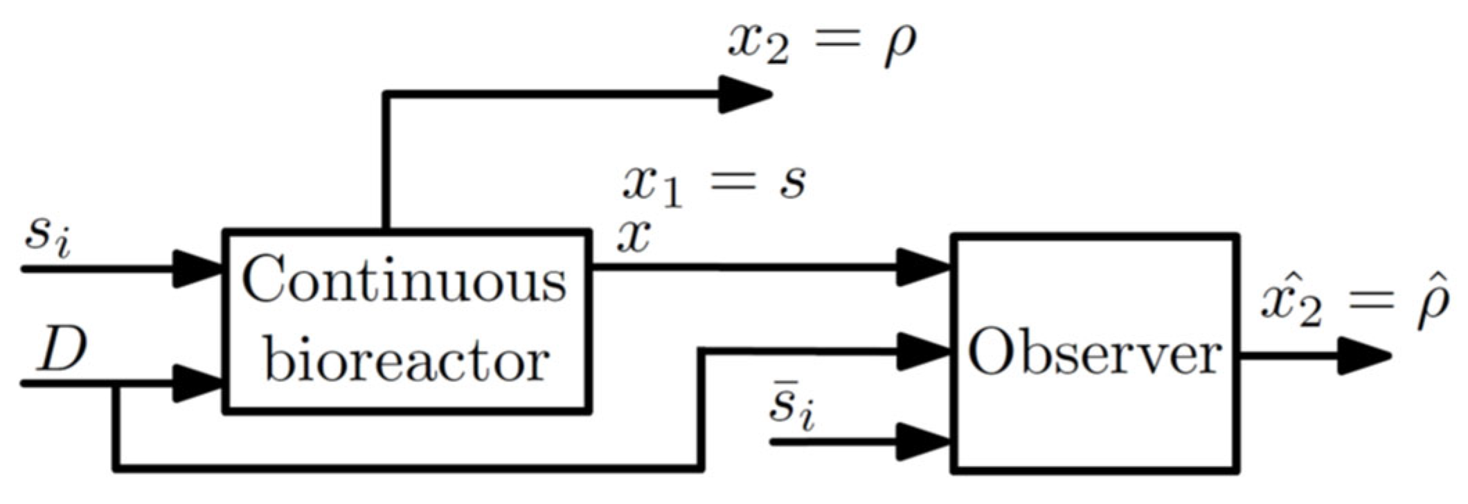
5. Application to Microalgae Bioreactor
5.1. First Example: Estimation of Substrate Uptake Rate
- −
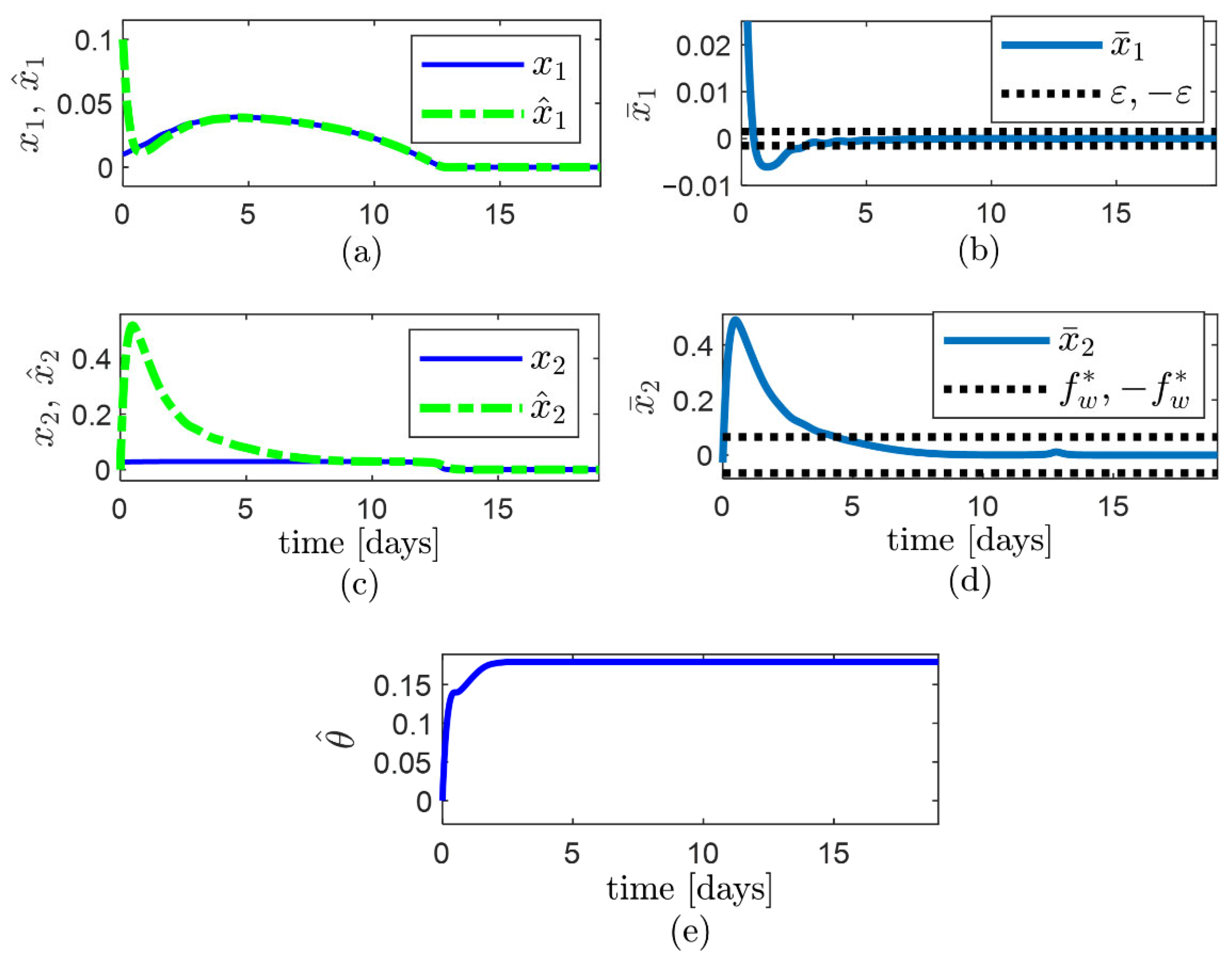
- The observer error converges faster than .
- −
- The observer error converges asymptotically to the compact set and remains inside for approx. (Figure 3a,b).
- −
- −
- The low width of is owed to the small values of and .
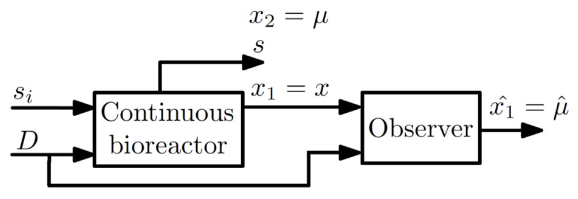
5.2. Second Example: Estimation of Biomass Growth Rate
- −
- The observer error converges faster than .
- −
- The observer error enters to the compact set at 4.92 days and remains inside afterward (Figure 6a,b).
- −
- −
- A low width of is achieved by choosing , values on the basis of the proposed algorithm.
6. Discussion and Conclusions
6.1. Discussion
- −
- The main contributions over closely related studies of the stability of state observers are:
- −
- Ci. The width of the convergence region of the observer error for the unknown state is expressed in terms of the interaction between the observer parameters and the disturbance in terms of the observer error dynamics. Then, the user defines the desired estimation accuracy by properly setting the observer parameters in accordance with the aforementioned relationship.
- −
- Cii. The properties and limits of this width are determined; it was found that this width has a minimum point and a vertical asymptote with respect to one of the observer parameters, and their coordinates were determined. Thus, the highest accuracy of the state estimation is obtained by setting the observer parameters equal or similar to the coordinates of the minimum.
- −
- The main challenges encountered in this research work are:
- −
- Choosing the idea of contributions Ci and Cii as the core topics of the paper required identifying contributions and limitations of high-quality works addressing observer design and stability analysis, mainly [23,25]. This implied a deep understanding of all the mathematical developments involved in the stability analysis, and also the advantages, disadvantages, and limitations of the observer and its stability properties.
6.2. Conclusions
Author Contributions
Funding
Institutional Review Board Statement
Informed Consent Statement
Data Availability Statement
Acknowledgments
Conflicts of Interest
References
- Reis de Souza, A.; Gouzé, J.L.; Efimov, D.; Polyakov, A. Robust Adaptive Estimation in the Competitive Chemostat. Comput. Chem. Eng. 2020, 142, 107030. [Google Scholar] [CrossRef]
- Zalai, D.; Kopp, J.; Kozma, B.; Küchler, M.; Herwig, C.; Kager, J. Microbial Technologies for Biotherapeutics Production: Key Tools for Advanced Biopharmaceutical Process Development and Control. Drug Discov. Today Technol. 2020, 38, 9–24. [Google Scholar] [CrossRef] [PubMed]
- Torres Zúñiga, I.; Villa-Leyva, A.; Vargas, A.; Buitrón, G. Experimental Validation of Online Monitoring and Optimization Strategies Applied to a Biohydrogen Production Dark Fermenter. Chem. Eng. Sci. 2018, 190, 48–59. [Google Scholar] [CrossRef]
- Lyubenova, V.N.; Ignatova, M.N. On-Line Estimation of Physiological States for Monitoring and Control of Bioprocesses. AIMS Bioeng. 2017, 4, 93–112. [Google Scholar] [CrossRef]
- Zeinali, S.; Shahrokhi, M. Observer-Based Singularity Free Nonlinear Controller for Uncertain Systems Subject to Input Saturation. Eur. J. Control 2020, 52, 49–58. [Google Scholar] [CrossRef]
- Ibáñez, F.; Saa, P.A.; Bárzaga, L.; Duarte-Mermoud, M.A.; Fernández-Fernández, M.; Agosin, E.; Pérez-Correa, J.R. Robust Control of Fed-Batch High-Cell Density Cultures: A Simulation-Based Assessment. Comput. Chem. Eng. 2021, 155, 107545. [Google Scholar] [CrossRef]
- Nuñez, S.; Garelli, F.; de Battista, H. Closed-Loop Growth-Rate Regulation in Fed-Batch Dual-Substrate Processes with Additive Kinetics Based on Biomass Concentration Measurement. J. Process Control 2016, 44, 14–22. [Google Scholar] [CrossRef]
- Jamilis, M.; Garelli, F.; de Battista, H. Growth Rate Maximization in Fed-Batch Processes Using High Order Sliding Controllers and Observers Based on Cell Density Measurement. J. Process Control 2018, 68, 23–33. [Google Scholar] [CrossRef]
- Lara-Cisneros, G.; Femat, R.; Dochain, D. An Extremum Seeking Approach via Variable-Structure Control for Fed-Batch Bioreactors with Uncertain Growth Rate. J. Process Control 2014, 24, 663–671. [Google Scholar] [CrossRef]
- Robles-Magdaleno, J.L.; Rodríguez-Mata, A.E.; Farza, M.; M’Saad, M. A Filtered High Gain Observer for a Class of Non Uniformly Observable Systems—Application to a Phytoplanktonic Growth Model. J. Process Control 2020, 87, 68–78. [Google Scholar] [CrossRef]
- Noll, P.; Henkel, M. History and Evolution of Modeling in Biotechnology: Modeling & Simulation, Application and Hardware Performance. Comput. Struct. Biotechnol. J. 2020, 18, 3309–3323. [Google Scholar] [CrossRef]
- Jamilis, M.; Garelli, F.; Mozumder, M.S.I.; Castañeda, T.; de Battista, H. Modeling and Estimation of Production Rate for the Production Phase of Non-Growth-Associated High Cell Density Processes. Bioprocess Biosyst. Eng. 2015, 38, 1903–1914. [Google Scholar] [CrossRef] [PubMed]
- Jin, Z.; Wang, Z.; Zhang, X. Cooperative Control Problem of Takagi-Sugeno Fuzzy Multiagent Systems via Observer Based Distributed Adaptive Sliding Mode Control. J. Franklin Inst. 2022, 359, 3405–3426. [Google Scholar] [CrossRef]
- Guo, R.; Feng, J.; Wang, J.; Zhao, Y. Leader-Following Successive Lag Consensus of Nonlinear Multi-Agent Systems via Observer-Based Event-Triggered Control. J. Franklin Inst. 2022. [Google Scholar] [CrossRef]
- Xiao, Y.; Che, W.W. Neural-Networks-Based Event-Triggered Consensus Tracking Control for Nonlinear MASs with DoS Attacks. Neurocomputing 2022, 501, 451–462. [Google Scholar] [CrossRef]
- Miranda-Colorado, R. Observer-Based Saturated Proportional Derivative Control of Perturbed Second-Order Systems: Prescribed Input and Velocity Constraints. ISA Trans. 2022, 122, 336–345. [Google Scholar] [CrossRef]
- Borkar, A.; Patil, P.M. Super Twisting Observer Based Full Order Sliding Mode Control. Int. J. Dyn. Control 2021, 9, 1653–1659. [Google Scholar] [CrossRef]
- ben Tarla, L.; Bakhti, M.; Bououlid Idrissi, B. Implementation of Second Order Sliding Mode Disturbance Observer for a One-Link Flexible Manipulator Using Dspace Ds1104. SN Appl. Sci. 2020, 2, 485. [Google Scholar] [CrossRef]
- Byun, G.; Kikuuwe, R. An Improved Sliding Mode Differentiator Combined with Sliding Mode Filter for Estimating First and Second-Order Derivatives of Noisy Signals. Int. J. Control Autom. Syst. 2020, 18, 3001–3014. [Google Scholar] [CrossRef]
- Liu, W.; Chen, S.; Huang, H. Double Closed-Loop Integral Terminal Sliding Mode for a Class of Underactuated Systems Based on Sliding Mode Observer. Int. J. Control Autom. Syst. 2020, 18, 339–350. [Google Scholar] [CrossRef]
- Besançon, G.; Voda, A.; Popescu, A. Closed-Loop-Based Observer Approach for Tunneling Current Parameter Estimation in an Experimental STM. Mechatronics 2022, 83, 102743. [Google Scholar] [CrossRef]
- Hu, Q.; Jiang, B.; Zhang, Y. Observer-Based Output Feedback Attitude Stabilization for Spacecraft With Finite-Time Convergence. IEEE Trans. Control Syst. Technol. 2019, 27, 781–789. [Google Scholar] [CrossRef]
- Coutinho, D.; Vargas, A.; Feudjio, C.; Benavides, M.; Wouwer, A. vande A Robust Approach to the Design of Super-Twisting Observers—Application to Monitoring Microalgae Cultures in Photo-Bioreactors. Comput. Chem. Eng. 2019, 121, 46–56. [Google Scholar] [CrossRef]
- Rincón, A.; Hoyos, F.E.; Restrepo, G.M. Design and Evaluation of a Robust Observer Using Dead-Zone Lyapunov Functions—Application to Reaction Rate Estimation in Bioprocesses. Fermentation 2022, 8, 173. [Google Scholar] [CrossRef]
- Kicki, P.; Łakomy, K.; Lee, K.M.B. Tuning of Extended State Observer with Neural Network-Based Control Performance Assessment. Eur. J. Control 2022, 64, 100609. [Google Scholar] [CrossRef]
- Wang, P.; Zhang, X.; Zhu, J. Online Performance-Based Adaptive Fuzzy Dynamic Surface Control for Nonlinear Uncertain Systems Under Input Saturation. IEEE Trans. Fuzzy Syst. 2019, 27, 209–220. [Google Scholar] [CrossRef]
- Madonski, R.; Shao, S.; Zhang, H.; Gao, Z.; Yang, J.; Li, S. General Error-Based Active Disturbance Rejection Control for Swift Industrial Implementations. Control Eng. Pract. 2019, 84, 218–229. [Google Scholar] [CrossRef]
- Shi, S.; Lu, J.; Hu, Y.; Sun, Y. Robust Output-Feedback SOSM Control Subject to Unmatched Disturbances and Its Application: A Fixed-Time Observer-Based Method. Nonlinear Anal. Hybrid Syst. 2022, 45, 101210. [Google Scholar] [CrossRef]
- Hans, S.; Joseph, F.O.M. Control of a Flexible Bevel-Tipped Needle Using Super-Twisting Controller Based Sliding Mode Observer. ISA Trans. 2021, 109, 186–198. [Google Scholar] [CrossRef]
- Meng, R.; Chen, S.; Hua, C.; Qian, J.; Sun, J. Disturbance Observer-Based Output Feedback Control for Uncertain QUAVs with Input Saturation. Neurocomputing 2020, 413, 96–106. [Google Scholar] [CrossRef]
- Abadi, A.S.S.; Hosseinabadi, P.A.; Mekhilef, S. Fuzzy Adaptive Fixed-Time Sliding Mode Control with State Observer for A Class of High-Order Mismatched Uncertain Systems. Int. J. Control Autom. Syst. 2020, 18, 2492–2508. [Google Scholar] [CrossRef]
- Tang, Z.-L.; Tee, K.P.; He, W. Tangent Barrier Lyapunov Functions for the Control of Output-Constrained Nonlinear Systems. IFAC Proc. Vol. 2013, 46, 449–455. [Google Scholar] [CrossRef]
- Rozgonyi, S.; Hangos, K.M.; Szederkényi, G. Determining the Domain of Attraction of Hybrid Non–Linear Systems Using Maximal Lyapunov Functions. Kybernetika 2010, 46, 19–37. [Google Scholar]
- Sankar, K.; Thakre, N.; Singh, S.M.; Jana, A.K. Sliding Mode Observer Based Nonlinear Control of a PEMFC Integrated with a Methanol Reformer. Energy 2017, 139, 1126–1143. [Google Scholar] [CrossRef]
- Valenciaga, F.; Inthamoussou, F.A. A Novel PV-MPPT Method Based on a Second Order Sliding Mode Gradient Observer. Energy Convers. Manag. 2018, 176, 422–430. [Google Scholar] [CrossRef]
- Zhang, L.; Wang, Z.; Li, S.; Ding, S.; Du, H. Universal Finite-Time Observer Based Second-Order Sliding Mode Control for DC-DC Buck Converters with Only Output Voltage Measurement. J. Franklin Inst. 2020, 357, 11863–11879. [Google Scholar] [CrossRef]
- Muñoz-Tamayo, R.; Martinon, P.; Bougaran, G.; Mairet, F.; Bernard, O. Getting the Most out of It: Optimal Experiments for Parameter Estimation of Microalgae Growth Models. J. Process Control 2014, 24, 991–1001. [Google Scholar] [CrossRef] [Green Version]


Publisher’s Note: MDPI stays neutral with regard to jurisdictional claims in published maps and institutional affiliations. |
© 2022 by the authors. Licensee MDPI, Basel, Switzerland. This article is an open access article distributed under the terms and conditions of the Creative Commons Attribution (CC BY) license (https://creativecommons.org/licenses/by/4.0/).
Share and Cite
Rincón, A.; Hoyos, F.E.; Candelo-Becerra, J.E. A Simplified Algorithm for Setting the Observer Parameters for Second-Order Systems with Persistent Disturbances Using a Robust Observer. Sensors 2022, 22, 6988. https://doi.org/10.3390/s22186988
Rincón A, Hoyos FE, Candelo-Becerra JE. A Simplified Algorithm for Setting the Observer Parameters for Second-Order Systems with Persistent Disturbances Using a Robust Observer. Sensors. 2022; 22(18):6988. https://doi.org/10.3390/s22186988
Chicago/Turabian StyleRincón, Alejandro, Fredy E. Hoyos, and John E. Candelo-Becerra. 2022. "A Simplified Algorithm for Setting the Observer Parameters for Second-Order Systems with Persistent Disturbances Using a Robust Observer" Sensors 22, no. 18: 6988. https://doi.org/10.3390/s22186988