
An Improved Spatiotemporal Data Fusion Method for Snow-Covered Mountain Areas Using Snow Index and Elevation Information
 ,
,  ,
,
Abstract
:1. Introduction
2. Materials
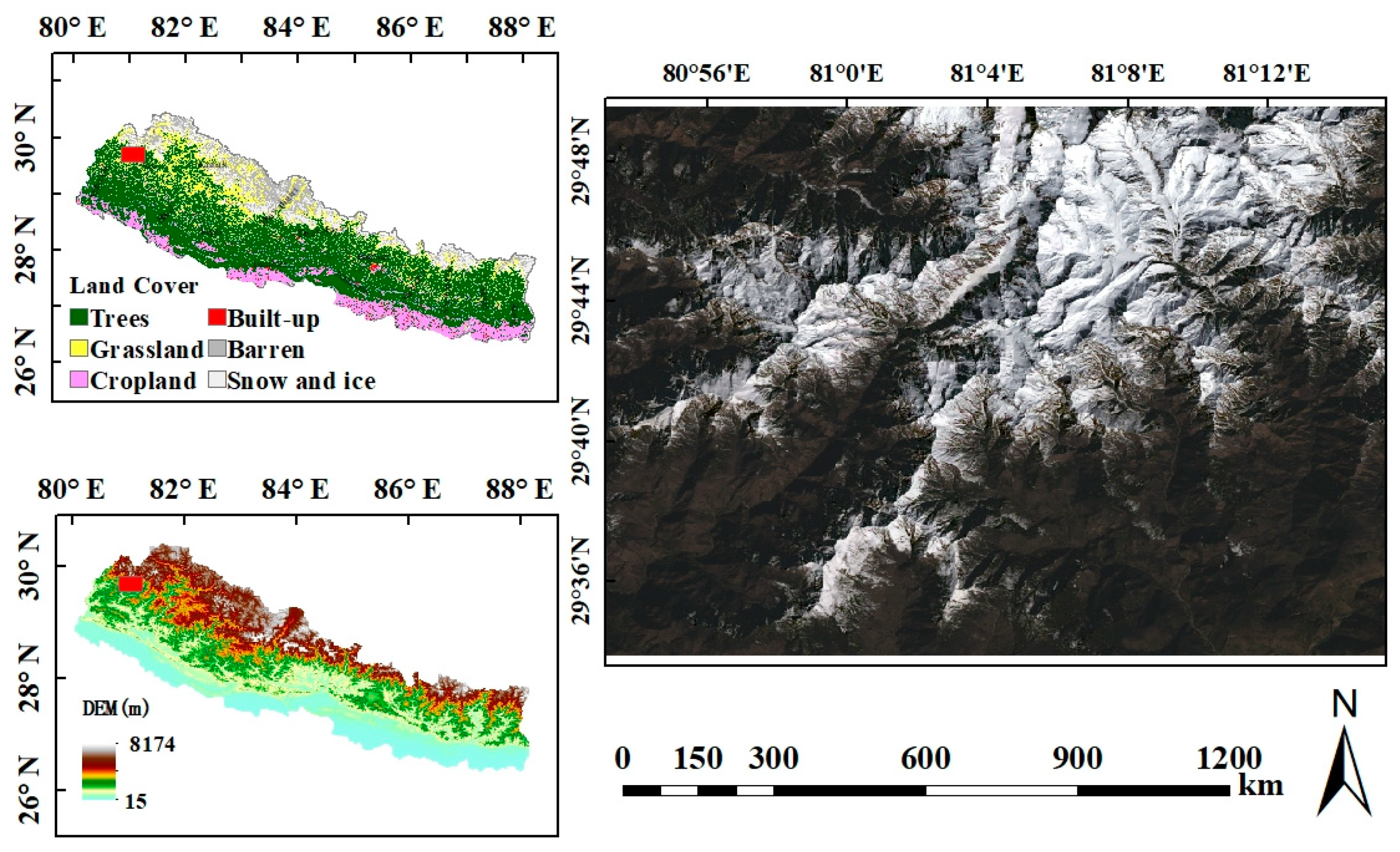
2.1. Study Area
2.2. Satellite Data and Preprocessing
3. Methods
3.1. Description of the Improved ESTARFM
- (1)
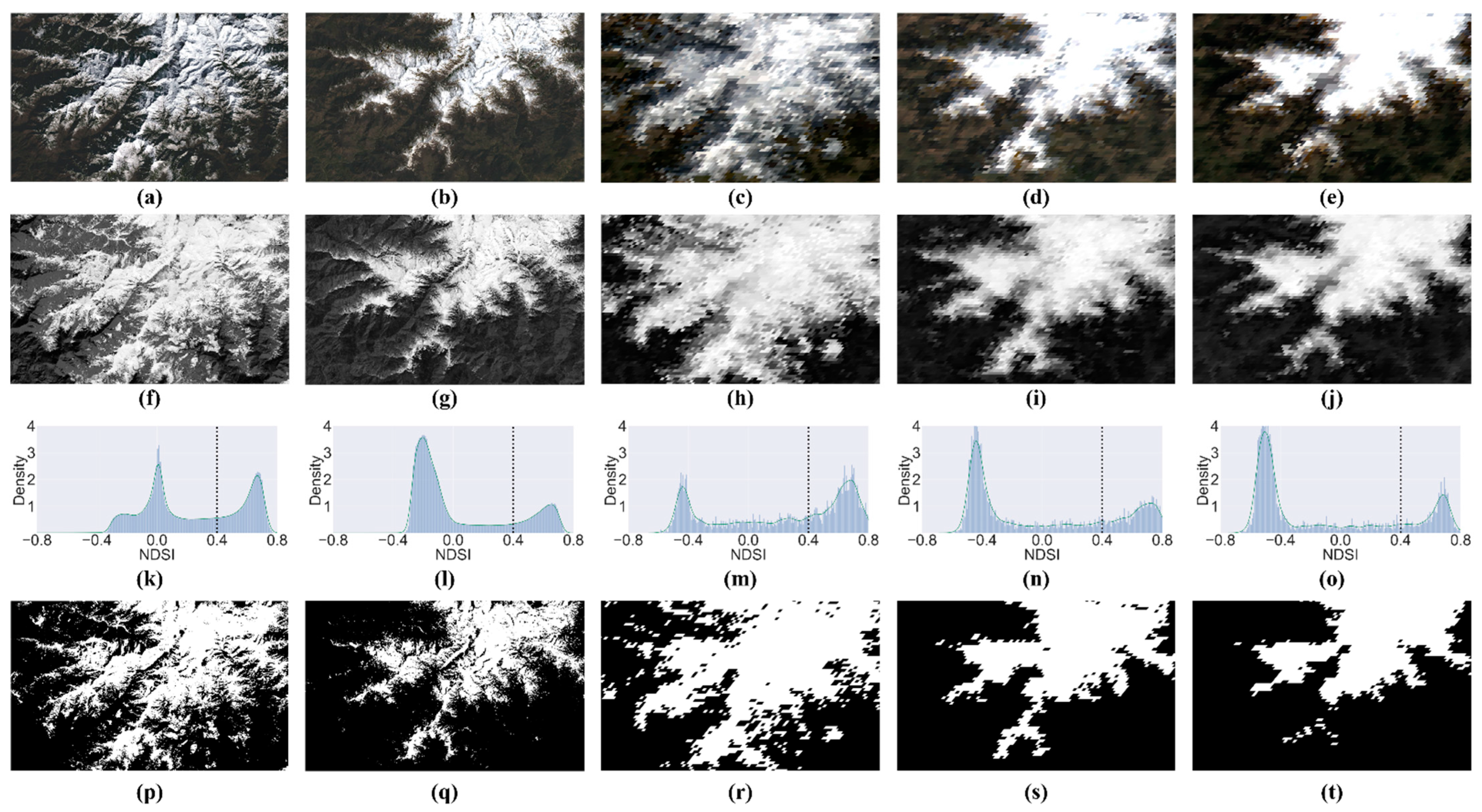
- Simulate snow cover based on NDSI at the base date. The normalized difference snow index (NDSI) is widely used for snow identification by taking advantage of the spectral characteristics that snow has high reflectance in the green band and low reflectance in the short-wave infrared band. Based on this, the ratio of the two bands is calculated to highlight the characteristics of snow from others [53], and the calculation equation is as follows:where is the reflectance of the green band, is the reflectance of the SWIR2 band.Firstly, by analyzing the NDSI distribution histogram and the true surface reflectance, the frequency histogram has two peaks, where the one with high values indicates the snow area and the one with low values indicates the non-snow area. Secondly, the NDSI threshold was determined by experimenting with different NDSI threshold values between the two peaks. Thirdly, the pixels with NDSI smaller than the threshold are considered as non-snow pixels and marked as 0, and those with NDSI larger than the threshold are considered as snow pixels and marked as 1. The experimental details are shown in Section 3.2, and the equation is as follows:where is the threshold to mask the snow-covered map, ( is the coordinate of the th pixel, is the base date, can be either or , is the snow-covered mask, with 1 indicating snow pixels and 0 indicating non-snow pixels.
- (2)
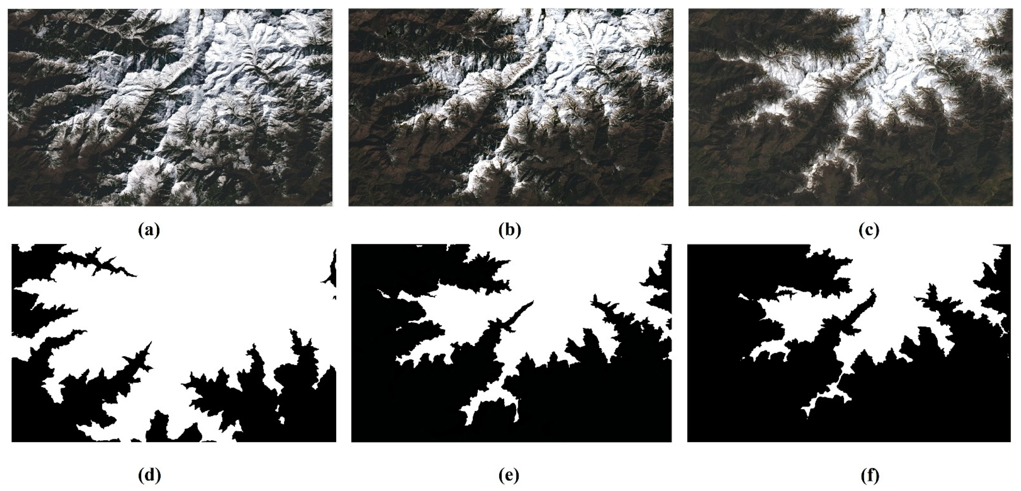
- Simulate snow cover based on DEM at the target date. The elevation is an important factor affecting the spatiotemporal distribution of the snow cover in mountainous areas [54,55,56,57,58,59]. The temperature at high altitudes is low, which is suitable for snow accumulation; meanwhile, the relatively high temperatures at lower altitudes cause snow to melt faster. The distribution of snow is strongly correlated with the elevation. Therefore, the combination of NDSI products and DEM is an effective approach for studying the spatial and temporal distribution of snow in mountain areas. Firstly, the coarse snow-covered borders are extracted from MODIS NDSI by using the local binary pattern (LBP) operator [67]. Then, the DEM values located at the boundaries are counted, and the threshold value of DEM is obtained. Thirdly, the pixels with DEM smaller than the threshold are considered non-snow pixels and marked as 0, and those with DEM larger than the threshold are considered snow pixels and marked as 1. The details are shown in Section 3.3, and the equation is as follows:where is the threshold of DEM to classify snow and non-snow pixels, is the mask obtained by thresholding at the target date, with 1 indicating snow pixels and 0 indicating non-snow pixels.
- (3)
- Select similar pixels. ESTARFM selects similar pixels based on spectral similarity [42]. The threshold is determined by the standard deviation of a population of pixels from the base image with a high spatial resolution. The improved method differs from ESTARFM in that it does not calculate thresholds based on the whole image but calculates the threshold for the snow and non-snow pixels separately to reduce errors in selecting similar pixels. Meanwhile, more similar pixels have more similar NDSI values, so NDSI is used as an additional condition to improve the accuracy of selecting similar pixels. Finally, similar pixels are selected based on spectral and NDSI differences. The equation is as follows:where is the spectral reflectance of fine images, is the size of the searching window, is the standard deviation of reflectance for band , is the estimated number of classes. Flag means the pixels marked as snow or non-snow, with flag = 1 indicating snow pixels and flag = 0 indicating non-snow pixels. is the threshold for non-snow or snow pixels, and is the threshold based on NDSI standard deviation.
- (4)
- Calculate weights and the conversion coefficient. The weight calculation in ESTARFM involves spectral, temporal, and spatial distances. Similarly, in iESTARFM, the spectral distance is calculated using the correlation coefficient between the fine image and the coarse image at . The spatial distance is calculated using the geographic distance between the similar pixels and target pixels. The temporal distance is calculated as the spectral difference between two coarse images. The conversion coefficient is the ratio of the change in the pure pixels in the fine image to the change in pixels in the coarse image, and it is calculated by a linear regression model. iESTARFM adds NDSI to the weight calculation to reduce the error of snow and non-snow identification. The weights equation is defined as follows:where is the spectral correlation coefficient for the th pixel, is the spatial distance, is the expected value, is the spatial distance, is the variance, is the spatial distance, is the normalized reciprocal of weight, and is the normalized weight.
- (5)
- Predict the target pixels. The prediction of the target pixels can be divided into two cases. Case 1: the pixels are marked with the same type at ,, and , indicating the type has not changed, so the target pixels can be calculated based on and . Case 2: the pixels are marked with the same type only on one date as , indicating that there is a change, so the target pixels are predicted based on the pixels marked with the same type. The equation is as follows:where is the snow-covered mask obtained by calculating the NDSI threshold, and is the snow-covered mask obtained by calculating the DEM threshold. is the predicted surface reflectance of the target pixels, is the prediction result calculated from the base image at time , and is the prediction result calculated from the base image at time .
3.2. Simulate Snow Cover Based on NDSI at the Base Date
3.3. Simulate Snow Cover Based on DEM at the Target Date
3.4. Data Quality Evaluation Metrics
4. Results
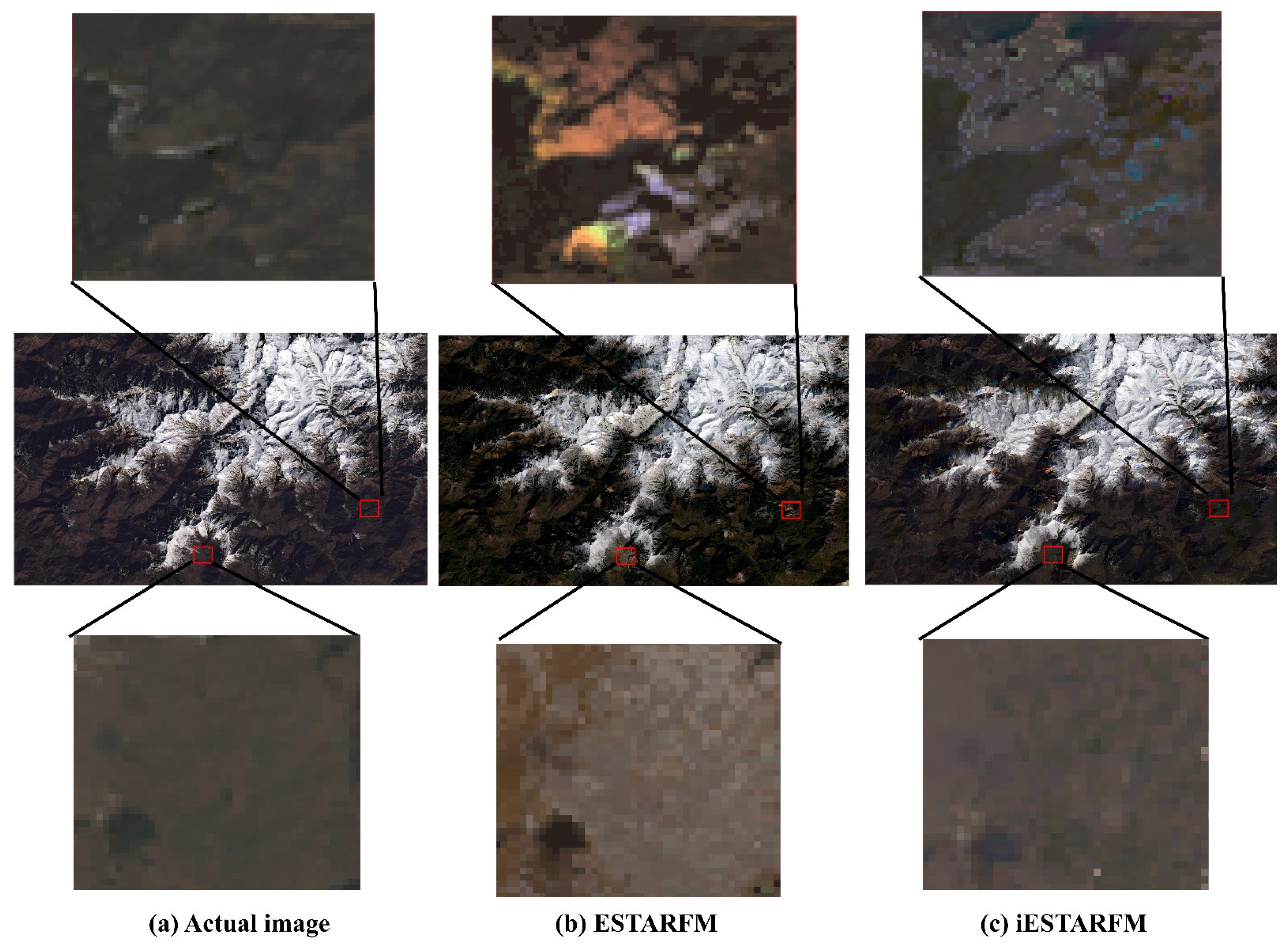
4.1. Qualitative Comparison
4.2. Quantitative Comparison
5. Discussion
6. Conclusions
Author Contributions
Funding
Institutional Review Board Statement
Informed Consent Statement
Data Availability Statement
Acknowledgments
Conflicts of Interest
References
- Pradhananga, D.; Pomeroy, J.W. Diagnosing changes in glacier hydrology from physical principles using a hydrological model with snow redistribution, sublimation, firnification and energy balance ablation algorithms. J. Hydrol. 2022, 608, 127545. [Google Scholar] [CrossRef]
- Guo, S.; Du, P.; Xia, J.; Tang, P.; Wang, X.; Meng, Y.; Wang, H. Spatiotemporal changes of glacier and seasonal snow fluctuations over the Namcha Barwa–Gyala Peri massif using object-based classification from Landsat time series. ISPRS J. Photogramm. Remote Sens. 2021, 177, 21–37. [Google Scholar] [CrossRef]
- Jin, H.; Chen, X.; Zhong, R.; Wu, P.; Ju, Q.; Zeng, J.; Yao, T. Extraction of snow melting duration and its spatiotemporal variations in the Tibetan Plateau based on MODIS product. Adv. Space Res. 2022, 70, 15–34. [Google Scholar] [CrossRef]
- Ahluwalia, R.S.; Rai, S.P.; Meetei, P.N.; Kumar, S.; Sarangi, S.; Chauhan, P.; Karakoti, I. Spatial-diurnal variability of snow/glacier melt runoff in glacier regime river valley: Central Himalaya, India. Quat. Int. 2021, 585, 183–194. [Google Scholar] [CrossRef]
- You, Q.; Cai, Z.; Pepin, N.; Chen, D.; Ahrens, B.; Jiang, Z.; Wu, F.; Kang, S.; Zhang, R.; Wu, T. Warming amplification over the Arctic Pole and Third Pole: Trends, mechanisms and consequences. Earth-Sci. Rev. 2021, 217, 103625. [Google Scholar] [CrossRef]
- Guo, D.; Wang, H. The significant climate warming in the northern Tibetan Plateau and its possible causes. Int. J. Climatol. 2012, 32, 1775–1781. [Google Scholar] [CrossRef]
- Wu, G.; Liu, Y.; Zhang, Q.; Duan, A.; Wang, T.; Wan, R.; Liu, X.; Li, W.; Wang, Z.; Liang, X. The influence of mechanical and thermal forcing by the Tibetan Plateau on Asian climate. J. Hydrometeorol. 2007, 8, 770–789. [Google Scholar] [CrossRef] [Green Version]
- Zhang, H.; Immerzeel, W.W.; Zhang, F.; de Kok, R.J.; Chen, D.; Yan, W. Snow cover persistence reverses the altitudinal patterns of warming above and below 5000 m on the Tibetan Plateau. Sci. Total Environ. 2022, 803, 149889. [Google Scholar] [CrossRef]
- Chen, Y.; Ge, Y.; Heuvelink, G.B.M.; An, R.; Chen, Y. Object-Based Superresolution Land-Cover Mapping From Remotely Sensed Imagery. IEEE Trans. Geosci. Remote Sens. 2018, 56, 328–340. [Google Scholar] [CrossRef]
- Hansen, M.C.; Potapov, P.V.; Moore, R.; Hancher, M.; Turubanova, S.A.; Tyukavina, A.; Thau, D.; Stehman, S.V.; Goetz, S.J.; Loveland, T.R. High-resolution global maps of 21st-century forest cover change. Science 2013, 342, 850–853. [Google Scholar] [CrossRef]
- Gong, P.; Li, X.; Zhang, W. 40-Year (1978–2017) human settlement changes in China reflected by impervious surfaces from satellite remote sensing. Sci. Bull. 2019, 64, 756–763. [Google Scholar] [CrossRef] [Green Version]
- Chen, Y.; Shi, K.; Ge, Y.; Zhou, Y. Spatiotemporal Remote Sensing Image Fusion Using Multiscale Two-Stream Convolutional Neural Networks. IEEE Trans. Geosci. Remote Sens. 2022, 60, 1–12. [Google Scholar] [CrossRef]
- Kakareka, S.; Kukharchyk, T.; Kurman, P. Trace and major elements in surface snow and fresh water bodies of the Marguerite Bay Islands, Antarctic Peninsula. Polar Sci. 2022, 32, 100792. [Google Scholar] [CrossRef]
- Yan, D.; Ma, N.; Zhang, Y. Development of a fine-resolution snow depth product based on the snow cover probability for the Tibetan Plateau: Validation and spatial–temporal analyses. J. Hydrol. 2022, 604, 127027. [Google Scholar] [CrossRef]
- Wang, X.; Wu, C.; Peng, D.; Gonsamo, A.; Liu, Z. Snow cover phenology affects alpine vegetation growth dynamics on the Tibetan Plateau: Satellite observed evidence, impacts of different biomes, and climate drivers. Agric. For. Meteorol. 2018, 256–257, 61–74. [Google Scholar] [CrossRef]
- Gao, F.; Masek, J.; Schwaller, M.; Hall, F. On the blending of the Landsat and MODIS surface reflectance: Predicting daily Landsat surface reflectance. IEEE Trans. Geosci. Remote Sens. 2006, 44, 2207–2218. [Google Scholar]
- De Gregorio, L.; Callegari, M.; Marin, C.; Zebisch, M.; Bruzzone, L.; Demir, B.; Strasser, U.; Marke, T.; Gunther, D.; Nadalet, R.; et al. A Novel Data Fusion Technique for Snow Cover Retrieval. IEEE J. Sel. Top. Appl. Earth Obs. Remote Sens. 2019, 12, 2873–2888. [Google Scholar] [CrossRef] [Green Version]
- Ju, J.; Roy, D.P. The availability of cloud-free Landsat ETM+ data over the conterminous United States and globally. Remote Sens. Environ. 2008, 112, 1196–1211. [Google Scholar] [CrossRef]
- Li, J.; Li, Y.; He, L.; Chen, J.; Plaza, A. Spatio-temporal fusion for remote sensing data: An overview and new benchmark. Sci. China Inf. Sci. 2020, 63, 140301. [Google Scholar] [CrossRef] [Green Version]
- Hilker, T.; Wulder, M.A.; Coops, N.C.; Linke, J.; McDermid, G.; Masek, J.G.; Gao, F.; White, J.C. A new data fusion model for high spatial- and temporal-resolution mapping of forest disturbance based on Landsat and MODIS. Remote Sens. Environ. 2009, 113, 1613–1627. [Google Scholar] [CrossRef]
- Zhang, B.; Zhang, L.; Xie, D.; Yin, X.; Liu, C.; Liu, G. Application of Synthetic NDVI Time Series Blended from Landsat and MODIS Data for Grassland Biomass Estimation. Remote Sens. 2016, 8, 10. [Google Scholar] [CrossRef]
- Jia, K.; Liang, S.; Wei, X.; Yao, Y.; Su, Y.; Jiang, B.; Wang, X. Land Cover Classification of Landsat Data with Phenological Features Extracted from Time Series MODIS NDVI Data. Remote Sens. 2014, 6, 11518–11532. [Google Scholar] [CrossRef] [Green Version]
- Chen, B.; Huang, B.; Xu, B. Multi-source remotely sensed data fusion for improving land cover classification. ISPRS J. Photogramm. Remote Sens. 2017, 124, 27–39. [Google Scholar] [CrossRef]
- Dhillon, M.S.; Dahms, T.; Kübert-Flock, C.; Steffan-Dewenter, I.; Zhang, J.; Ullmann, T. Ullmann, Spatiotemporal Fusion Modelling Using STARFM: Examples of Landsat 8 and Sentinel-2 NDVI in Bavaria. Remote Sens. 2022, 14, 677. [Google Scholar] [CrossRef]
- Zhou, J.; Chen, J.; Chen, X.; Zhu, X.; Qiu, Y.; Song, H.; Rao, Y.; Zhang, C.; Cao, X.; Cui, X. Sensitivity of six typical spatiotemporal fusion methods to different influential factors: A comparative study for a normalized difference vegetation index time series reconstruction. Remote Sens. Environ. 2021, 252, 112130. [Google Scholar] [CrossRef]
- Zhu, X.L.; Cai, F.Y.; Tian, J.Q.; Williams, T.K.A. Spatiotemporal Fusion of Multisource Remote Sensing Data: Literature Survey, Taxonomy, Principles, Applications, and Future Directions. Remote Sens. 2018, 10, 527. [Google Scholar] [CrossRef] [Green Version]
- Zhu, X.; Zhan, W.; Zhou, J.; Chen, X.; Liang, Z.; Xu, S.; Chen, J. A novel framework to assess all-round performances of spatiotemporal fusion models. Remote Sens. Environ. 2022, 274, 113002. [Google Scholar] [CrossRef]
- Chen, B.; Huang, B.; Xu, B. Comparison of Spatiotemporal Fusion Models: A Review. Remote Sens. 2015, 7, 1798–1835. [Google Scholar] [CrossRef] [Green Version]
- Ping, B.; Meng, Y.; Su, F. An enhanced spatial and temporal adaptive reflectance fusion model based on optimal window. In Proceedings of the 2017 IEEE International Geoscience and Remote Sensing Symposium (IGARSS), Fort Worth, TX, USA, 23–28 July 2017. [Google Scholar] [CrossRef]
- Emelyanova, I.; Mcvicar, T.; Niel, T.V.; Li, L.; Dijk, A.V. On Blending Landsat-MODIS Surface Reflectances in Two Landscapes with Contrasting Spectral, Spatial and Temporal Dynamics; CSIRO: Canberra, Australia, 2012. [Google Scholar] [CrossRef]
- Zhukov, B.; Oertel, D.; Lanzl, F.; Reinhackel, G. Unmixing-based multisensor multiresolution image fusion. IEEE Trans. Geosci. Remote Sens. 1999, 37, 1212–1226. [Google Scholar] [CrossRef]
- Wu, M.; Niu, Z.; Wang, C.; Wu, C.; Wang, L. Use of MODIS and Landsat time series data to generate high-resolution temporal synthetic Landsat data using a spatial and temporal reflectance fusion model. J. Appl. Remote Sens. 2012, 6, 063507. [Google Scholar] [CrossRef]
- Xue, J.; Leung, Y.; Fung, T. A Bayesian data fusion approach to spatio-temporal fusion of remotely sensed images. Remote Sens. 2017, 9, 1310. [Google Scholar] [CrossRef] [Green Version]
- Jia, D.; Song, C.; Cheng, C.; Shen, S.; Ning, L.; Hui, C. A novel deep learning-based spatiotemporal fusion method for combining satellite images with different resolutions using a two-stream convolutional neural network. Remote Sens. 2020, 12, 698. [Google Scholar] [CrossRef] [Green Version]
- Wang, X.; Wang, X. Spatiotemporal fusion of remote sensing image based on deep learning. J. Sens. 2020, 2020, 8873079. [Google Scholar] [CrossRef]
- Zhu, X.; Helmer, E.H.; Gao, F.; Liu, D.; Chen, J.; Lefsky, M.A. A flexible spatiotemporal method for fusing satellite images with different resolutions. Remote Sens. Environ. 2016, 172, 165–177. [Google Scholar] [CrossRef]
- Jia, D.; Cheng, C.; Song, C.; Shen, S.; Ning, L.; Zhang, T. A hybrid deep learning-based spatiotemporal fusion method for combining satellite images with different resolutions. Remote Sens. 2021, 13, 645. [Google Scholar] [CrossRef]
- Gevaert, C.M.; García-Haro, F.J. A comparison of STARFM and an unmixing-based algorithm for Landsat and MODIS data fusion. Remote Sens. Environ. 2015, 156, 34–44. [Google Scholar] [CrossRef]
- Ma, J.; Zhang, W.; Marinoni, A.; Gao, L.; Zhang, B. Performance assessment of ESTARFM with different similar-pixel identification schemes. J. Appl. Remote Sens. 2018, 12, 025017. [Google Scholar] [CrossRef]
- Liu, M.; Liu, X.; Dong, X.; Zhao, B.; Zou, X.; Wu, L.; Wei, H. An improved spatiotemporal data fusion method using surface heterogeneity information based on estarfm. Remote Sens. 2020, 12, 3673. [Google Scholar] [CrossRef]
- Knauer, K.; Gessner, U.; Fensholt, R.; Kuenzer, C. An ESTARFM fusion framework for the generation of large-scale time series in cloud-prone and heterogeneous landscapes. Remote Sens. 2016, 8, 425. [Google Scholar] [CrossRef]
- Zhu, X.; Chen, J.; Gao, F.; Chen, X.; Masek, J.G. An enhanced spatial and temporal adaptive reflectance fusion model for complex heterogeneous regions. Remote Sens. Environ. 2010, 114, 2610–2623. [Google Scholar] [CrossRef]
- Ghosh, R.; Gupta, P.K.; Tolpekin, V.; Srivastav, S.K. An enhanced spatiotemporal fusion method—Implications for coal fire monitoring using satellite imagery. Int. J. Appl. Earth Obs. Geoinf. 2020, 88, 102056. [Google Scholar] [CrossRef]
- Bazrgar Bajestani, A.; Akhoondzadeh Hanzaei, M. ESTARFM Model for Fusion of LST Products of MODIS and ASTER Sensors to Retrieve the High Resolution Land Surface Temperature Map. J. Geomat. Sci. Technol. 2018, 7, 147–161. [Google Scholar]
- Chen, M.; Li, C.; Guan, Y.; Zhou, J.; Wang, D.; Luo, Z. Generation and application of high temporal and spatial resolution images of regional farmland based on ESTARFM model. Acta Agron. Sin. 2019, 45, 1099–1110. [Google Scholar] [CrossRef]
- Da Silva, B.B.; Mercante, E.; Kusminski, D.; Cattani, C.E.V.; Mendes, I.d.S.; Caon, I.L.; Ganascini, D.; Prior, M. Synthetic images to map daily evapotranspiration in field scale using SEBAL model and ESTARFM algorithm. Aust. J. Crop Sci. 2020, 14, 504–509. [Google Scholar] [CrossRef]
- Liu, W.; Zeng, Y.; Li, S.; Pi, X.; Huang, W. An improved spatiotemporal fusion approach based on multiple endmember spectral mixture analysis. Sensors 2019, 19, 2443. [Google Scholar] [CrossRef] [Green Version]
- Zhang, H.; Sun, Y.; Shi, W.; Guo, D.; Zheng, N. An object-based spatiotemporal fusion model for remote sensing images. Eur. J. Remote Sens. 2021, 54, 86–101. [Google Scholar] [CrossRef]
- Liu, M.; Liu, X.; Wu, L.; Zou, X.; Jiang, T.; Zhao, B. A modified spatiotemporal fusion algorithm using phenological information for predicting reflectance of paddy rice in southern China. Remote Sens. 2018, 10, 772. [Google Scholar] [CrossRef] [Green Version]
- Wang, X.; Xie, H. New methods for studying the spatiotemporal variation of snow cover based on combination products of MODIS Terra and Aqua. J. Hydrol. 2009, 371, 192–200. [Google Scholar] [CrossRef]
- Tarigan, D.G.; Isa, S.M. A PSNR Review of ESTARFM Cloud Removal Method with Sentinel 2 and Landsat 8 Combination. Int. J. Adv. Comput. Sci. Appl. 2021, 12, 189–198. [Google Scholar] [CrossRef]
- Nietupski, T.C.; Kennedy, R.E.; Temesgen, H.; Kerns, B.K. Spatiotemporal image fusion in Google Earth Engine for annual estimates of land surface phenology in a heterogenous landscape. Int. J. Appl. Earth Obs. Geoinf. 2021, 99, 102323. [Google Scholar] [CrossRef]
- Lin, J.; Feng, X.; Xiao, P.; Li, H.; Wang, J.; Li, Y. Comparison of snow indexes in estimating snow cover fraction in a mountainous area in northwestern China. IEEE Geosci. Remote Sens. Lett. 2012, 9, 725–729. [Google Scholar] [CrossRef]
- Pandey, A.C.; Ghosh, S.; Nathawat, M.S.; Tiwari, R.K. Area Change and Thickness Variation over Pensilungpa Glacier (J&K) using Remote Sensing. J. Indian Soc. Remote Sens. 2012, 40, 245–255. [Google Scholar] [CrossRef]
- Bhambri, R.; Bolch, T. Glacier mapping: A review with special reference to the Indian Himalayas. Prog. Phys. Geogr. Earth Environ. 2009, 33, 672–704. [Google Scholar] [CrossRef] [Green Version]
- Rignot, E.; Rivera, A.; Casassa, G. Contribution of the Patagonia Icefields of South America to sea level rise. Science 2003, 302, 434–437. [Google Scholar] [CrossRef] [PubMed] [Green Version]
- Surazakov, A.B.; Aizen, V.B. Estimating volume change of mountain glaciers using SRTM and map-based topographic data. Ieee Trans. Geosci. Remote Sens. 2006, 44, 2991–2995. [Google Scholar] [CrossRef]
- Berthier, E.; Arnaud, Y.; Kumar, R.; Ahmad, S.; Wagnon, P.; Chevallier, P. Remote sensing estimates of glacier mass balances in the Himachal Pradesh (Western Himalaya, India). Remote Sens. Environ. 2007, 108, 327–338. [Google Scholar] [CrossRef] [Green Version]
- Bolch, T.; Kamp, U. Glacier Mapping in High Mountains Using DEMs, Landsat and ASTER Data. 2005. Available online: https://www.semanticscholar.org/paper/Glacier-mapping-in-high-mountains-using-DEMs%2C-and-Bolch-Kamp/123fcb9070bb27cce3b899bd53cbe787931bf25a (accessed on 10 May 2020).
- Campbell, B. Biodiversity, livelihoods and struggles over sustainability in Nepal. Landsc. Res. 2018, 43, 1056–1067. [Google Scholar] [CrossRef] [Green Version]
- Paudel, B.; Zhang, Y.-l.; Li, S.-c.; Liu, L.-s.; Wu, X.; Khanal, N.R. Review of studies on land use and land cover change in Nepal. J. Mt. Sci. 2016, 13, 643–660. [Google Scholar] [CrossRef]
- Shrestha, A.B.; Joshi, S.P. Snow cover and glacier change study in Nepalese Himalaya using remote sensing and geographic information system. J. Hydrol. Meteorol. 2009, 6, 26–36. [Google Scholar] [CrossRef]
- Emelyanova, I.V.; McVicar, T.R.; van Niel, T.G.; Li, L.T.; van Dijk, A.I.J.M. Assessing the accuracy of blending Landsat–MODIS surface reflectances in two landscapes with contrasting spatial and temporal dynamics: A framework for algorithm selection. Remote Sens. Environ. 2013, 133, 193–209. [Google Scholar] [CrossRef]
- Vermote, E.; Justice, C.; Claverie, M.; Franch, B. Preliminary analysis of the performance of the Landsat 8/OLI land surface reflectance product. Remote Sens. Environ. 2016, 185, 46–56. [Google Scholar] [CrossRef] [PubMed]
- Vermote, E. MYD09A1 MODIS/Aqua Surface Reflectance 8-Day L3 Global 500m SIN Grid V006 [Data set]. 2015. Available online: https://lpdaac.usgs.gov/products/myd09a1v006/ (accessed on 10 May 2020).
- Zhao, S.; Cheng, W.; Zhou, C.; Chen, X.; Zhang, S.; Zhou, Z.; Liu, H.; Chai, H. Accuracy assessment of the ASTER GDEM and SRTM3 DEM: An example in the Loess Plateau and North China Plain of China. Int. J. Remote Sens. 2011, 32, 8081–8093. [Google Scholar] [CrossRef]
- Zhu, C.; Wang, R. Local multiple patterns based multiresolution gray-scale and rotation invariant texture classification. Inf. Sci. 2012, 187, 93–108. [Google Scholar] [CrossRef]
- Zhou, Y.; Jiang, H.; Wang, Z.; Yang, X.; Geng, E. Assessment of Four Typical Topographic Corrections in Landsat Tm Data for Snow Cover Areas. Int. Arch. Photogramm. Remote Sens. Spat. Inf. Sci. 2016, 41, 157–162. [Google Scholar] [CrossRef] [Green Version]
- Pan, Z.; Ma, W.; Guo, J.; Lei, B. Super-resolution of single remote sensing image based on residual dense backprojection networks. IEEE Trans. Geosci. Remote Sens. 2019, 57, 7918–7933. [Google Scholar] [CrossRef]
- Johnson, A.P.; Baker, C.L. First-and second-order information in natural images: A filter-based approach to image statistics. JOSA A 2004, 21, 913–925. [Google Scholar] [CrossRef]
- Qian, D.; Gungor, O.; Jie, S. Performance evaluation for pan-sharpening techniques. In Proceedings of the IEEE International Geoscience and Remote Sensing Symposium 2005, IGARSS ’05, Seoul, Korea, 29 July 2005. [Google Scholar] [CrossRef]
- Li, X.; Foody, G.M.; Boyd, D.S.; Ge, Y.; Zhang, Y.; Du, Y.; Ling, F. SFSDAF: An enhanced FSDAF that incorporates sub-pixel class fraction change information for spatio-temporal image fusion. Remote Sens. Environ. 2020, 237, 111537. [Google Scholar] [CrossRef]
- Yuhas, R.H.; Goetz, A.F.; Boardman, J.W. Discrimination among semi-arid landscape endmembers using the spectral angle mapper (SAM) algorithm. In Proceedings of the JPL, Summaries of the Third Annual JPL Airborne Geoscience Workshop, Pasadena, CA, USA, 1–5 June 1992; Volume 1: AVIRIS Workshop. [Google Scholar]
- Ponomarenko, N.; Ieremeiev, O.; Lukin, V.; Egiazarian, K.; Carli, M. Modified image visual quality metrics for contrast change and mean shift accounting. In Proceedings of the 2011 11th International Conference The Experience of Designing and Application of CAD Systems in Microelectronics (CADSM), Polyana, Ukraine, 23–25 February 2011. [Google Scholar]
- Li, W.; Cao, D.; Peng, Y.; Yang, C. MSNet: A multi-stream fusion network for remote sensing spatiotemporal fusion based on transformer and convolution. Remote Sens. 2021, 13, 3724. [Google Scholar] [CrossRef]
- Zhu, L.; Xiao, P.; Feng, X.; Zhang, X.; Wang, Z.; Jiang, L. Support vector machine-based decision tree for snow cover extraction in mountain areas using high spatial resolution remote sensing image. J. Appl. Remote Sens. 2014, 8, 084698. [Google Scholar] [CrossRef]
- Pepe, M.; Boschetti, L.; Brivio, P.A.; Rampini, A. Accuracy benefits of a fuzzy classifier in remote sensing data classification of snow. In Proceedings of the 2007 IEEE International Fuzzy Systems Conference, London, UK, 23–26 July 2007. [Google Scholar] [CrossRef]


| Band | Landsat 8 OLI | Bandwidth (nm) | MODIS | Bandwidth (nm) |
|---|---|---|---|---|
| Blue | Band 2 | 450–510 | Band 3 | 459–479 |
| Green | Band 3 | 530–590 | Band 4 | 545–565 |
| Red | Band 4 | 630–690 | Band 1 | 620–670 |
| Near Infrared | Band 5 | 850–880 | Band 2 | 841–876 |
| Short-Wave Infrared 1 (SWIR1) | Band 6 | 1570–1650 | Band 6 | 1628–1652 |
| Short-Wave Infrared 2 (SWIR2) | Band 7 | 2110–2290 | Band 7 | 2105–2155 |
| Data Type | Spatial Resolution | Temporal Resolution | Acquisition Date | Expression | Use | Percentage of Snow | Percentage of Cloud |
|---|---|---|---|---|---|---|---|
| Landsat8 OLI | 30 m | 16 days | 2020/01/11 | Base Image | 39.07 | <5 | |
| 30 m | 2020/02/12 | Evaluation | 25.44 | <5 | |||
| 30 m | 2020/03/31 | Base Image | 22.71 | <5 | |||
| MODIS | 500 m | daily | 2020/01/09 | Base Image | 48.44 | <5 | |
| 500 m | 2020/02/10 | Base Image | 30.72 | <5 | |||
| 500 m | 2020/03/29 | Base Image | 25.30 | <5 |
| Metric Name | Equation | Variable Explanation |
|---|---|---|
| MSE | : the value of the ith pixel in the true image | |
| RMSE | : the value of the ith pixel in the predicted image | |
| r | the mean pixel values of the predicted image | |
| ERGAS | : the mean pixel values of the true image | |
| SSIM | : the variance of pixel values of the predicted image | |
| SAM | : the variance of pixel values of the true image | |
| PSNR | : constants N: the total number of pixels | |
| Edge | : the value of ith pixel in the moving window |
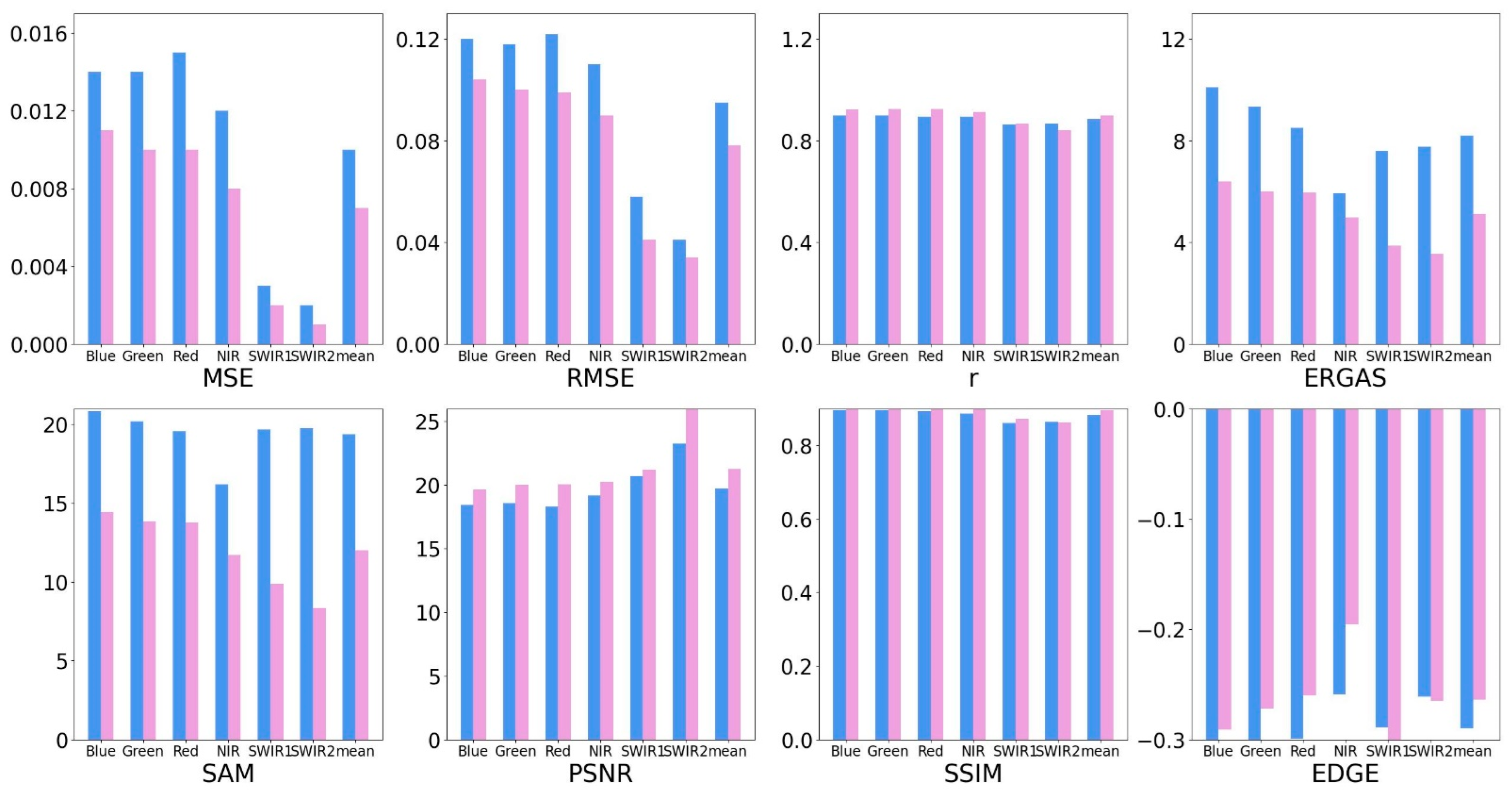
| Metrics | Method | Band | ||||||
|---|---|---|---|---|---|---|---|---|
| Blue | Green | Red | NIR | SWIR1 | SWIR2 | Average | ||
| MSE | ESTARFM | 0.014 | 0.014 | 0.015 | 0.012 | 0.003 | 0.002 | 0.010 |
| iESTARFM | 0.011 | 0.010 | 0.010 | 0.008 | 0.002 | 0.001 | 0.007 | |
| RMSE | ESTARFM | 0.120 | 0.118 | 0.122 | 0.110 | 0.058 | 0.041 | 0.095 |
| iESTARFM | 0.104 | 0.100 | 0.099 | 0.090 | 0.041 | 0.034 | 0.078 | |
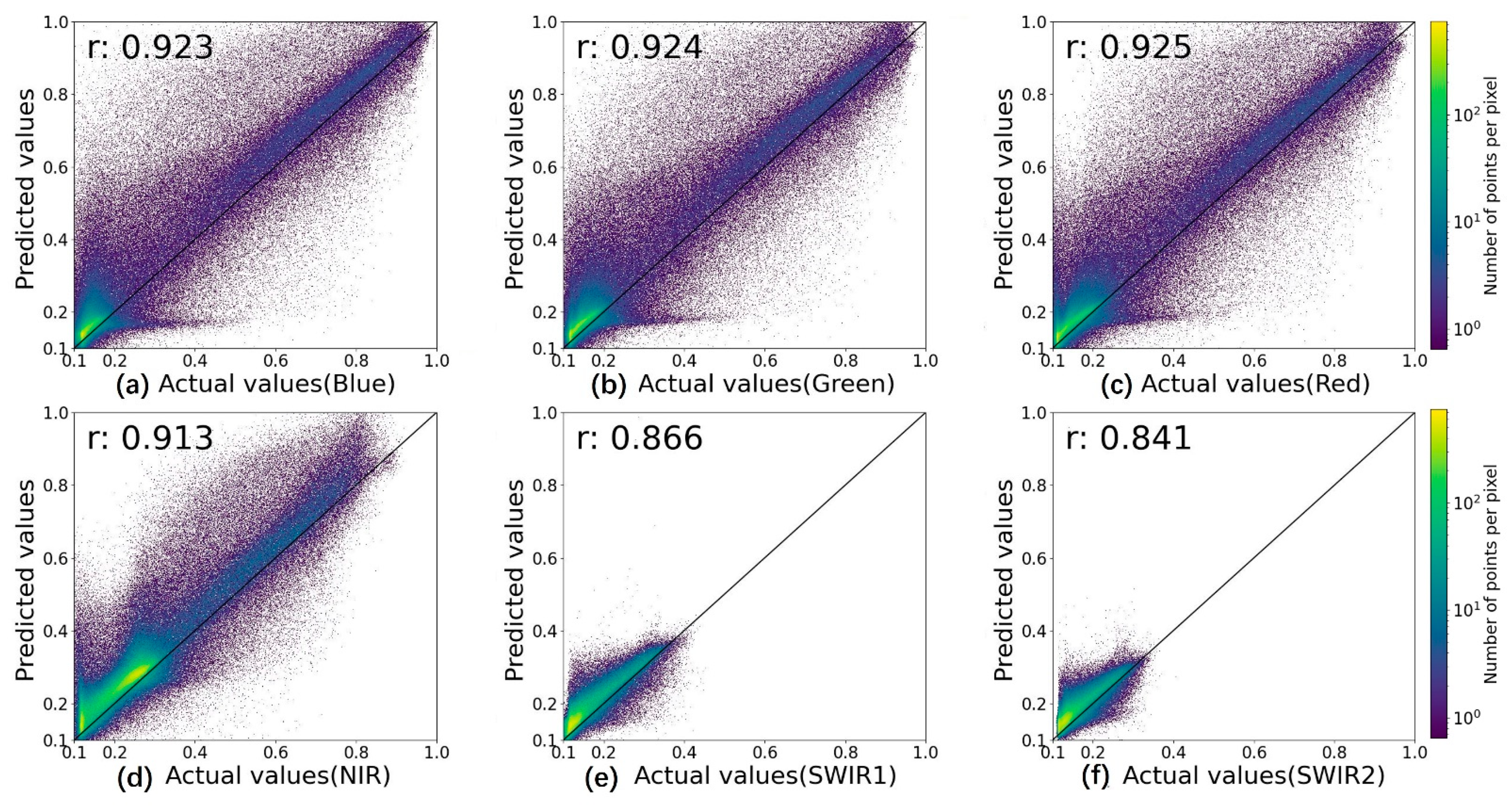
| r | ESTARFM | 0.898 | 0.898 | 0.895 | 0.894 | 0.864 | 0.867 | 0.886 |
| iESTARFM | 0.923 | 0.924 | 0.925 | 0.913 | 0.866 | 0.841 | 0.899 | |
| ERGAS | ESTARFM | 10.113 | 9.348 | 8.505 | 5.935 | 7.605 | 7.764 | 8.212 |
| iESTARFM | 6.389 | 6.013 | 5.964 | 4.985 | 3.881 | 3.555 | 5.131 | |
| SAM | ESTARFM | 20.825 | 20.195 | 19.567 | 16.188 | 19.675 | 19.75 | 19.367 |
| iESTARFM | 14.428 | 13.827 | 13.763 | 11.717 | 9.885 | 8.351 | 11.995 | |
| PSNR | ESTARFM | 18.422 | 18.569 | 18.291 | 19.162 | 20.708 | 23.263 | 19.736 |
| iESTARFM | 19.634 | 19.997 | 20.045 | 20.256 | 21.226 | 26.494 | 21.275 | |
| SSIM | ESTARFM | 0.896 | 0.896 | 0.893 | 0.887 | 0.861 | 0.865 | 0.883 |
| iESTARFM | 0.911 | 0.914 | 0.915 | 0.902 | 0.872 | 0.863 | 0.896 | |
| EDGE | ESTARFM | −0.328 | −0.307 | −0.299 | −0.259 | −0.289 | −0.261 | −0.29 |
| iESTARFM | −0.291 | −0.272 | −0.260 | −0.196 | −0.3 | −0.265 | −0.264 | |
Publisher’s Note: MDPI stays neutral with regard to jurisdictional claims in published maps and institutional affiliations. |
© 2022 by the authors. Licensee MDPI, Basel, Switzerland. This article is an open access article distributed under the terms and conditions of the Creative Commons Attribution (CC BY) license (https://creativecommons.org/licenses/by/4.0/).
Share and Cite
Gao, M.; Gu, X.; Liu, Y.; Zhan, Y.; Wei, X.; Yu, H.; Liang, M.; Weng, C.; Ding, Y. An Improved Spatiotemporal Data Fusion Method for Snow-Covered Mountain Areas Using Snow Index and Elevation Information. Sensors 2022, 22, 8524. https://doi.org/10.3390/s22218524
Gao M, Gu X, Liu Y, Zhan Y, Wei X, Yu H, Liang M, Weng C, Ding Y. An Improved Spatiotemporal Data Fusion Method for Snow-Covered Mountain Areas Using Snow Index and Elevation Information. Sensors. 2022; 22(21):8524. https://doi.org/10.3390/s22218524
Chicago/Turabian StyleGao, Min, Xingfa Gu, Yan Liu, Yulin Zhan, Xiangqin Wei, Haidong Yu, Man Liang, Chenyang Weng, and Yaozong Ding. 2022. "An Improved Spatiotemporal Data Fusion Method for Snow-Covered Mountain Areas Using Snow Index and Elevation Information" Sensors 22, no. 21: 8524. https://doi.org/10.3390/s22218524