
Learning with Weak Annotations for Robust Maritime Obstacle Detection

Abstract
1. Introduction
2. Related Work
2.1. Maritime Obstacle Detection
2.2. Reducing the Annotation Effort
3. Learning Segmentation by Scaffolding
3.1. Feature Warm-Up
3.1.1. Partial Labels from Weak Annotations
3.1.2. Training
3.2. Estimating Pseudo Labels from Features
3.3. Fine-Tuning with Dense Pseudo Labels
4. Results
4.1. Evaluation Protocol
4.2. Comparison with Full Supervision
4.3. Segmentation Quality
4.4. Comparison with Semi-Supervised Learning
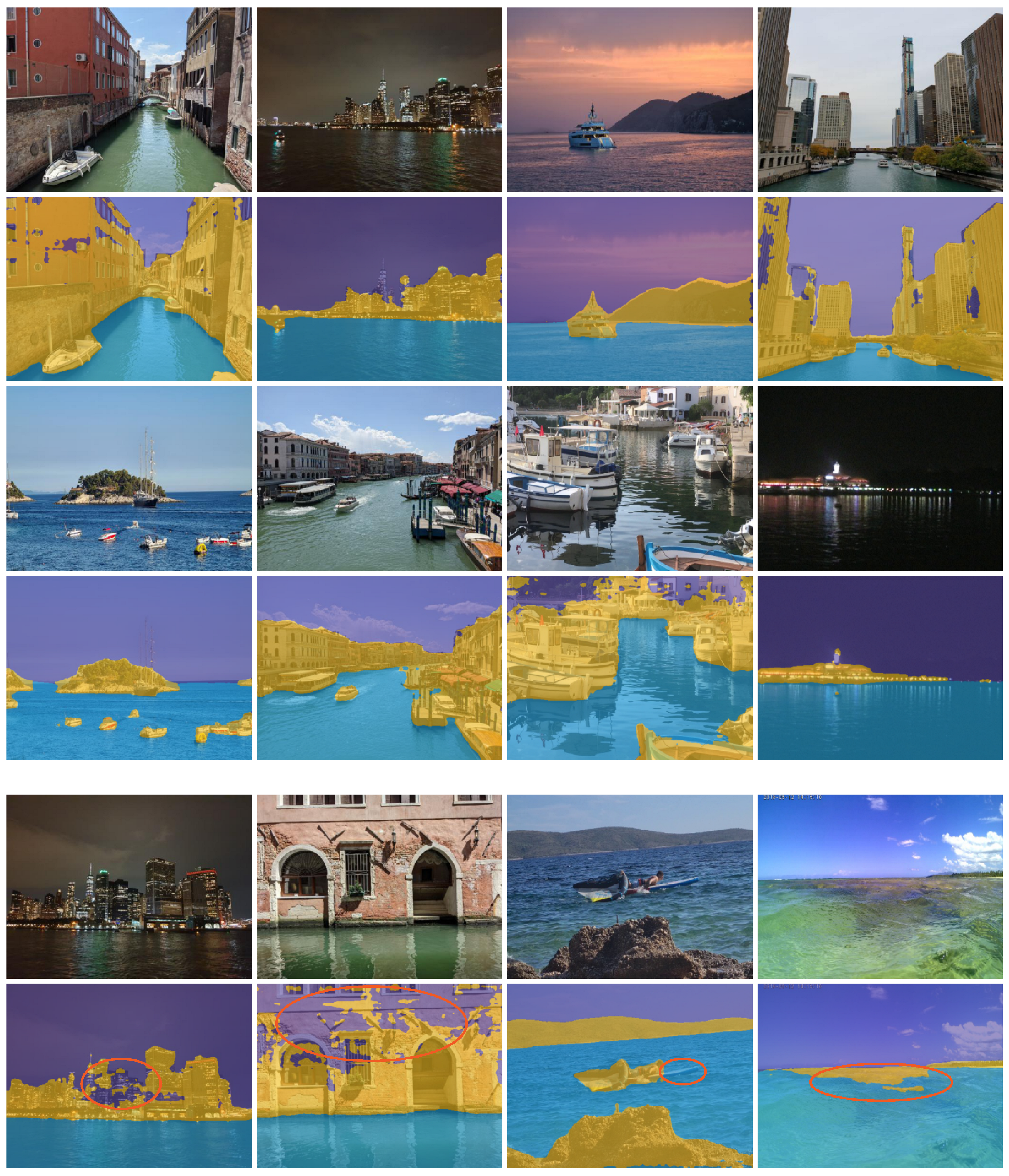
4.5. Cross-Domain Generalization
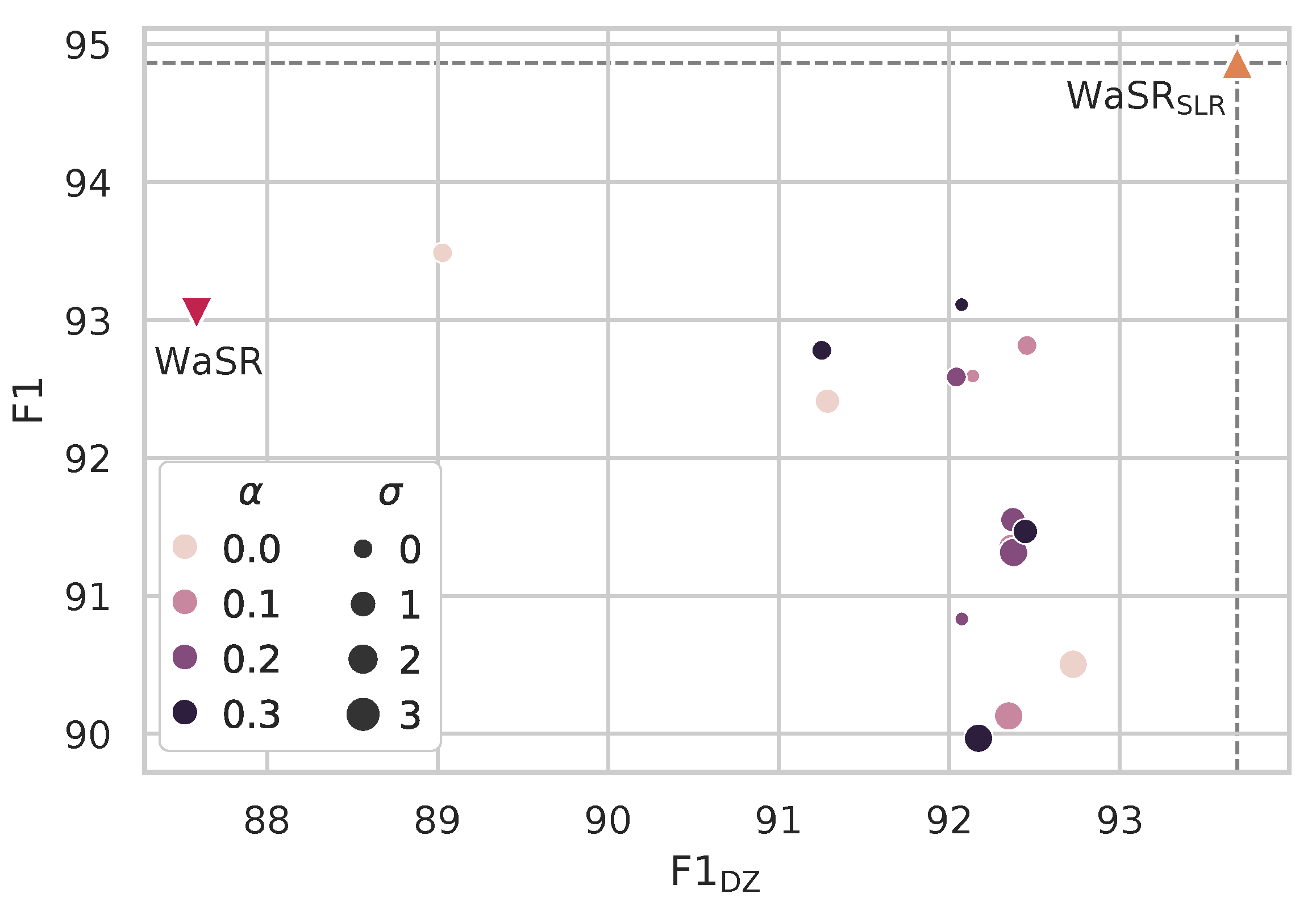
4.6. Ablation Study
4.7. Influence of SLR Iterations
4.8. Comparison with Label Smoothing
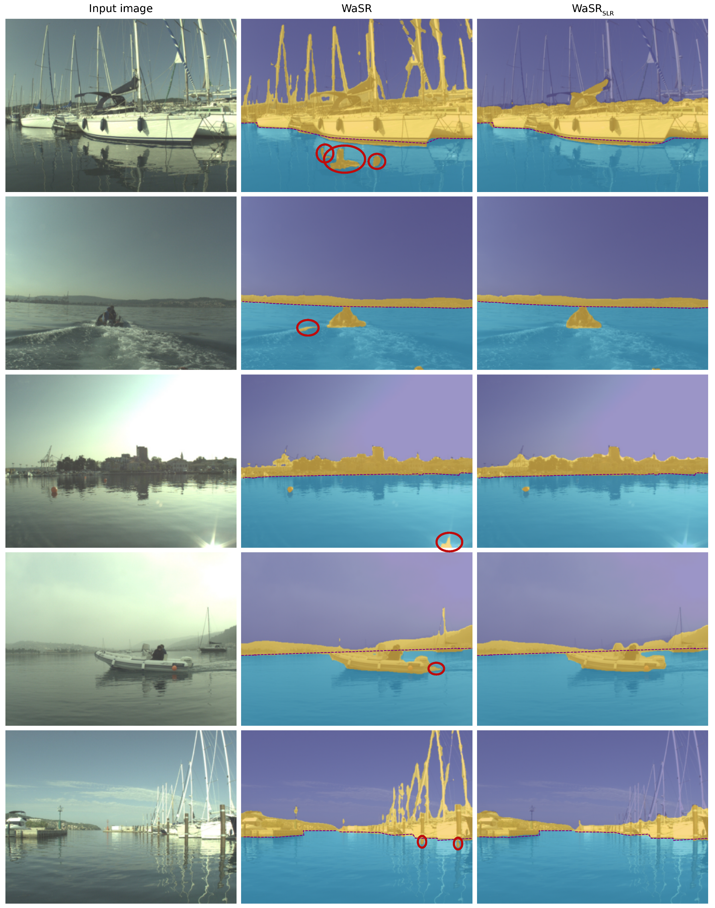
4.9. Qualitative Analysis
5. Conclusions
Author Contributions
Funding
Institutional Review Board Statement
Informed Consent Statement
Data Availability Statement
Conflicts of Interest
References
- Bovcon, B.; Muhovič, J.; Vranac, D.; Mozetič, D.; Perš, J.; Kristan, M. MODS—A USV-oriented Object Detection and Obstacle Segmentation Benchmark. IEEE Trans. Intell. Transp. Syst. 2021, 23, 13403–13418. [Google Scholar] [CrossRef]
- Bovcon, B.; Muhovič, J.; Perš, J.; Kristan, M. The MaSTr1325 Dataset for Training Deep USV Obstacle Detection Models. In Proceedings of the 2019 IEEE/RSJ International Conference on Intelligent Robots and Systems (IROS), Macau, China, 3–8 November 2019; pp. 3431–3438. [Google Scholar] [CrossRef]
- Maninis, K.K.; Caelles, S.; Pont-Tuset, J.; Van Gool, L. Deep Extreme Cut: From Extreme Points to Object Segmentation. In Proceedings of the IEEE Computer Society Conference on Computer Vision and Pattern Recognition, Salt Lake City, UT, USA, 18–23 June 2018. [Google Scholar] [CrossRef]
- Zhang, S.; Liew, J.H.; Wei, Y.; Wei, S.; Zhao, Y. Interactive Object Segmentation with Inside-Outside Guidance. In Proceedings of the 2020 IEEE/CVF Conference on Computer Vision and Pattern Recognition (CVPR), Seattle, WA, USA, 13–19 June 2020. [Google Scholar]
- Vu, T.H.; Jain, H.; Bucher, M.; Cord, M.; Pérez, P. ADVENT: Adversarial Entropy Minimization for Domain Adaptation in Semantic Segmentation. In Proceedings of the 2019 IEEE/CVF Conference on Computer Vision and Pattern Recognition (CVPR), Long Beach, CA, USA, 15–20 June 2019. [Google Scholar] [CrossRef]
- Yang, Y.; Soatto, S. FDA: Fourier Domain Adaptation for Semantic Segmentation. In Proceedings of the 2020 IEEE Computer Society Conference on Computer Vision and Pattern Recognition, Seattle, WA, USA, 13–19 June 2020; pp. 4084–4094. [Google Scholar] [CrossRef]
- Huo, X.; Xie, L.; He, J.; Yang, Z.; Zhou, W.; Li, H.; Tian, Q. ATSO: Asynchronous Teacher-Student Optimization for Semi-Supervised Image Segmentation. In Proceedings of the 2021 IEEE/CVF Conference on Computer Vision and Pattern Recognition (CVPR), Nashville, TN, USA, 20–25 June 2021; pp. 1235–1244. [Google Scholar]
- Mittal, S.; Tatarchenko, M.; Brox, T. Semi-Supervised Semantic Segmentation with High- In addition, Low-Level Consistency. IEEE Trans. Pattern Anal. Mach. Intell. 2019, 43, 1369–1379. [Google Scholar] [CrossRef] [PubMed]
- Li, Q.; Arnab, A.; Torr, P.H.S. Weakly- and Semi-Supervised Panoptic Segmentation. In Proceedings of the 15th European Conference on Computer Vision (ECCV), Munich, Germany, 8–14 September 2018; pp. 102–118. [Google Scholar]
- Wang, X.; Ma, H.; You, S. Deep Clustering for Weakly-Supervised Semantic Segmentation in Autonomous Driving Scenes. Neurocomputing 2020, 381, 20–28. [Google Scholar] [CrossRef]
- Žust, L.; Kristan, M. Learning Maritime Obstacle Detection from Weak Annotations by Scaffolding. In Proceedings of the 2022 IEEE/CVF Winter Conference on Applications of Computer Vision, Waikoloa, HI, USA, 4–8 January 2022; pp. 955–964. [Google Scholar] [CrossRef]
- Prasad, D.K.; Prasath, C.K.; Rajan, D.; Rachmawati, L.; Rajabally, E.; Quek, C. Object Detection in a Maritime Environment: Performance Evaluation of Background Subtraction Methods. IEEE Trans. Intell. Transp. Syst. 2019, 20, 1787–1802. [Google Scholar] [CrossRef]
- Wang, H.; Wei, Z. Stereovision Based Obstacle Detection System for Unmanned Surface Vehicle. In Proceedings of the 2013 IEEE International Conference on Robotics and Biomimetics (ROBIO), Shenzhen, China, 12–14 December 2013. [Google Scholar] [CrossRef]
- Kristan, M.; Kenk, V.S.; Kovačič, S.; Perš, J. Fast Image-Based Obstacle Detection from Unmanned Surface Vehicles. IEEE Trans. Cybern. 2016, 46, 641–654. [Google Scholar] [CrossRef]
- Bai, X.; Chen, Z.; Zhang, Y.; Liu, Z.; Lu, Y. Infrared Ship Target Segmentation Based on Spatial Information Improved FCM. IEEE Trans. Cybern. 2016, 46, 3259–3271. [Google Scholar] [CrossRef]
- Lee, S.J.; Roh, M.I.; Lee, H.W.; Ha, J.S.; Woo, I.G. Image-Based Ship Detection and Classification for Unmanned Surface Vehicle Using Real-Time Object Detection Neural Networks. In Proceedings of the International Offshore and Polar Engineering Conference, Sapporo, Japan, 10–15 June 2018. [Google Scholar]
- Moosbauer, S.; Konig, D.; Jakel, J.; Teutsch, M. A Benchmark for Deep Learning Based Object Detection in Maritime Environments. In Proceedings of the 2019 IEEE Computer Society Conference on Computer Vision and Pattern Recognition Workshops, Long Beach, CA, USA, 16–17 June 2019; pp. 916–925. [Google Scholar] [CrossRef]
- Yang, J.; Li, Y.; Zhang, Q.; Ren, Y. Surface Vehicle Detection and Tracking with Deep Learning and Appearance Feature. In Proceedings of the 2019 5th International Conference on Control, Automation and Robotics, Beijing, China, 19–22 April 2019. [Google Scholar] [CrossRef]
- Ren, S.; He, K.; Girshick, R.; Sun, J. Faster R-CNN: Towards Real-Time Object Detection with Region Proposal Networks. IEEE Trans. Pattern Anal. Mach. Intell. 2017, 39, 1137–1149. [Google Scholar] [CrossRef] [PubMed]
- Ma, L.; Xie, W.; Huang, H. Convolutional Neural Network Based Obstacle Detection for Unmanned Surface Vehicle. Math. Biosci. Eng. 2020, 17, 845–861. [Google Scholar] [CrossRef] [PubMed]
- Chen, L.C.; Papandreou, G.; Schroff, F.; Adam, H. Rethinking Atrous Convolution for Semantic Image Segmentation. arXiv 2017, arXiv:1706.05587. [Google Scholar]
- Yu, C.; Gao, C.; Wang, J.; Yu, G.; Shen, C.; Sang, N. BiSeNet V2: Bilateral Network with Guided Aggregation for Real-Time Semantic Segmentation. Int. J. Comput. Vis. 2021, 129, 3051–3068. [Google Scholar] [CrossRef]
- Cane, T.; Ferryman, J. Evaluating Deep Semantic Segmentation Networks for Object Detection in Maritime Surveillance. In Proceedings of the AVSS 2018—2018 15th IEEE International Conference on Advanced Video and Signal-Based Surveillance, Auckland, New Zealand, 27–30 November 2018. [Google Scholar] [CrossRef]
- Kim, H.; Koo, J.; Kim, D.; Park, B.; Jo, Y.; Myung, H.; Lee, D. Vision-Based Real-Time Obstacle Segmentation Algorithm for Autonomous Surface Vehicle. IEEE Access 2019, 7, 179420–179428. [Google Scholar] [CrossRef]
- Steccanella, L.; Bloisi, D.D.; Castellini, A.; Farinelli, A. Waterline and Obstacle Detection in Images from Low-Cost Autonomous Boats for Environmental Monitoring. Robot. Auton. Syst. 2020, 124, 103346. [Google Scholar] [CrossRef]
- Bovcon, B.; Kristan, M. WaSR–A Water Segmentation and Refinement Maritime Obstacle Detection Network. IEEE Trans. Cybern. 2021, 52, 12661–12674. [Google Scholar] [CrossRef] [PubMed]
- Qiao, D.; Liu, G.; Li, W.; Lyu, T.; Zhang, J. Automated Full Scene Parsing for Marine ASVs Using Monocular Vision. J. Intell. Robot. Syst. 2022, 104, 1–20. [Google Scholar] [CrossRef]
- Yao, L.; Kanoulas, D.; Ji, Z.; Liu, Y. ShorelineNet: An Efficient Deep Learning Approach for Shoreline Semantic Segmentation for Unmanned Surface Vehicles. In Proceedings of the 2021 IEEE/RSJ International Conference on Intelligent Robots and Systems (IROS 2021), Prague, Czech Republic, 27 September–1 October 2021. [Google Scholar]
- Ronneberger, O.; Fischer, P.; Brox, T. U-Net: Convolutional Networks for Biomedical Image Segmentation. In Medical Image Computing and Computer-Assisted Intervention—MICCAI 2015, Proceedings of the Lecture Notes in Computer Science (Including Subseries Lecture Notes in Artificial Intelligence and Lecture Notes in Bioinformatics); Lecture Notes in Computer Science; Springer: Cham, Switzerland, 2015; Volume 9351, pp. 234–241. [Google Scholar] [CrossRef]
- Prasad, D.K.; Rajan, D.; Rachmawati, L.; Rajabally, E.; Quek, C. Video Processing From Electro-Optical Sensors for Object Detection and Tracking in a Maritime Environment: A Survey. IEEE Trans. Intell. Transp. Syst. 2017, 18, 1993–2016. [Google Scholar] [CrossRef]
- Cheng, Y.; Jiang, M.; Zhu, J.; Liu, Y. Are We Ready for Unmanned Surface Vehicles in Inland Waterways? The USVInland Multisensor Dataset and Benchmark. IEEE Robot. Autom. Lett. 2021, 6, 3964–3970. [Google Scholar] [CrossRef]
- Hung, W.C.; Tsai, Y.H.; Liou, Y.T.; Lin, Y.Y.; Yang, M.H. Adversarial Learning for Semi-Supervised Semantic Segmentation. In Proceedings of the British Machine Vision Conference 2018, Newcastle, UK, 3–6 September 2018. [Google Scholar]
- Sae-ang, B.-i.; Kumwilaisak, W.; Kaewtrakulpong, P. Semi-Supervised Learning for Defect Segmentation with Autoencoder Auxiliary Module. Sensors 2022, 22, 2915. [Google Scholar] [CrossRef]
- Chan, L.; Hosseini, M.S.; Plataniotis, K.N. A Comprehensive Analysis of Weakly-Supervised Semantic Segmentation in Different Image Domains. Int. J. Comput. Vis. 2021, 129, 361–384. [Google Scholar] [CrossRef]
- Kim, W.S.; Lee, D.H.; Kim, T.; Kim, H.; Sim, T.; Kim, Y.J. Weakly Supervised Crop Area Segmentation for an Autonomous Combine Harvester. Sensors 2021, 21, 4801. [Google Scholar] [CrossRef]
- Papandreou, G.; Chen, L.C.; Murphy, K.; Yuille, A.L. Weakly- and Semi-Supervised Learning of a DCNN for Semantic Image Segmentation. In Proceedings of the 2015 IEEE International Conference on Computer Vision (ICCV), Santiago, Chile, 7–13 December 2015. [Google Scholar] [CrossRef]
- Durand, T.; Mordan, T.; Thome, N.; Cord, M. WILDCAT: Weakly Supervised Learning of Deep ConvNets for Image Classification, Pointwise Localization and Segmentation. In Proceedings of the 2017 IEEE Conference on Computer Vision and Pattern Recognition (CVPR), Honolulu, HI, USA, 21–26 July 2017; pp. 5957–5966. [Google Scholar] [CrossRef]
- Ahn, J.; Kwak, S. Learning Pixel-Level Semantic Affinity with Image-Level Supervision for Weakly Supervised Semantic Segmentation. In Proceedings of the 2018 IEEE/CVF Conference on Computer Vision and Pattern Recognition, Salt Lake City, UT, USA, 18–23 June 2018. [Google Scholar] [CrossRef]
- Wang, Y.; Zhang, J.; Kan, M.; Shan, S.; Chen, X. Self-Supervised Equivariant Attention Mechanism for Weakly Supervised Semantic Segmentation. In Proceedings of the 2020 IEEE/CVF Conference on Computer Vision and Pattern Recognition (CVPR), Seattle, WA, USA, 13–19 June 2020. [Google Scholar] [CrossRef]
- Wang, X.; Liu, S.; Ma, H.; Yang, M.H. Weakly-Supervised Semantic Segmentation by Iterative Affinity Learning. Int. J. Comput. Vis. 2020, 128, 1736–1749. [Google Scholar] [CrossRef]
- Adke, S.; Li, C.; Rasheed, K.M.; Maier, F.W. Supervised and Weakly Supervised Deep Learning for Segmentation and Counting of Cotton Bolls Using Proximal Imagery. Sensors 2022, 22, 3688. [Google Scholar] [CrossRef] [PubMed]
- Vernaza, P.; Chandraker, M. Learning Random-Walk Label Propagation for Weakly-Supervised Semantic Segmentation. In Proceedings of the 2017 IEEE Conference on Computer Vision and Pattern Recognition (CVPR), Honolulu, HI, USA, 21–26 July 2017. [Google Scholar] [CrossRef]
- Zhang, J.; Yu, X.; Li, A.; Song, P.; Liu, B.; Dai, Y. Weakly-Supervised Salient Object Detection via Scribble Annotations. In Proceedings of the 2020 IEEE/CVF Conference on Computer Vision and Pattern Recognition (CVPR), Seattle, WA, USA, 13–19 June 2020. [Google Scholar] [CrossRef]
- Chun, C.; Ryu, S.K. Road Surface Damage Detection Using Fully Convolutional Neural Networks and Semi-Supervised Learning. Sensors 2019, 19, 5501. [Google Scholar] [CrossRef] [PubMed]
- Akiva, P.; Dana, K.; Oudemans, P.; Mars, M. Finding Berries: Segmentation and Counting of Cranberries Using Point Supervision and Shape Priors. In Proceedings of the 2020 IEEE Computer Society Conference on Computer Vision and Pattern Recognition Workshops, Seattle, WA, USA, 14–19 June 2020. [Google Scholar] [CrossRef]
- Dai, J.; He, K.; Sun, J. BoxSup: Exploiting Bounding Boxes to Supervise Convolutional Networks for Semantic Segmentation. In Proceedings of the 2015 IEEE International Conference on Computer Vision (ICCV), Santiago, Chile, 7–13 December 2015. [Google Scholar]
- Kulharia, V.; Chandra, S.; Agrawal, A.; Torr, P.; Tyagi, A. Box2Seg: Attention Weighted Loss and Discriminative Feature Learning for Weakly Supervised Segmentation. In Computer Vision—ECCV 2020, Proceedings of the Lecture Notes in Computer Science (Including Subseries Lecture Notes in Artificial Intelligence and Lecture Notes in Bioinformatics); Lecture Notes in Computer Science; Springer: Cham, Switzerland, 2020; Volume 12372, pp. 290–308. [Google Scholar] [CrossRef]
- Hsu, C.C.; Hsu, K.J.; Tsai, C.C.; Lin, Y.Y.; Chuang, Y.Y. Weakly Supervised Instance Segmentation Using the Bounding Box Tightness Prior. In Proceedings of the Advances in Neural Information Processing Systems 32: Annual Conference on Neural Information Processing Systems 2019, Vancouver, BC, Canada, 8–14 December 2019. [Google Scholar]
- Tian, Z.; Shen, C.; Wang, X.; Chen, H. BoxInst: High-Performance Instance Segmentation with Box Annotations. In Proceedings of the 2021 IEEE/CVF Conference on Computer Vision and Pattern Recognition (CVPR), Nashville, TN, USA, 20–25 June 2021; pp. 5443–5452. [Google Scholar]
- Zhao, B.; Bhat, G.; Danelljan, M.; Van Gool, L.; Timofte, R. Generating Masks from Boxes by Mining Spatio-Temporal Consistencies in Videos. In Proceedings of the 2021 IEEE/CVF International Conference on Computer Vision, ICCV, Montreal, QC, Canada, 10–17 October 2021. [Google Scholar]
- Lin, T.Y.; Goyal, P.; Girshick, R.; He, K.; Dollar, P. Focal Loss for Dense Object Detection. IEEE Trans. Pattern Anal. Mach. Intell. 2020, 42, 318–327. [Google Scholar] [CrossRef] [PubMed]
- Yan, B.; Zhang, X.; Wang, D.; Lu, H.; Yang, X. Alpha-Refine: Boosting Tracking Performance by Precise Bounding Box Estimation. In Proceedings of the 2021 IEEE/CVF Conference on Computer Vision and Pattern Recognition (CVPR), Nashville, TN, USA, 20–25 June 2021; pp. 5289–5298. [Google Scholar]
- Lin, G.; Milan, A.; Shen, C.; Reid, I. RefineNet: Multi-path Refinement Networks for High-Resolution Semantic Segmentation. In Proceedings of the 30th IEEE Conference on Computer Vision and Pattern Recognition, Honolulu, HI, USA, 21–26 July 2017. [Google Scholar] [CrossRef]
- Chen, L.C.; Papandreou, G.; Kokkinos, I.; Murphy, K.; Yuille, A.L. DeepLab: Semantic Image Segmentation with Deep Convolutional Nets, Atrous Convolution, and Fully Connected CRFs. IEEE Trans. Pattern Anal. Mach. Intell. 2018, 40, 834–848. [Google Scholar] [CrossRef] [PubMed]
- Yu, C.; Wang, J.; Peng, C.; Gao, C.; Yu, G.; Sang, N. BiSeNet: Bilateral Segmentation Network for Real-Time Semantic Segmentation. In Computer Vision—ECCV 2018, Proceedings of the Lecture Notes in Computer Science (Including Subseries Lecture Notes in Artificial Intelligence and Lecture Notes in Bioinformatics); Lecture Notes in Computer Science; Springer: Cham, Switzerland, 2018; Volume 11217, pp. 334–349. [Google Scholar] [CrossRef]
- Islam, M.; Glocker, B. Spatially Varying Label Smoothing: Capturing Uncertainty from Expert Annotations. In Proceedings of the Information Processing in Medical Imaging, Virtual Event, 28– 30 June 2021; pp. 677–688. [Google Scholar]


| Model | Overall | Danger Zone (<15 m) | |||||
|---|---|---|---|---|---|---|---|
| Pr | Re | F1 | Pr | Re | F1 | ||
| RefineNet | 97.3 | 89.0 | 93.0 | 91.0 | 45.1 | 98.1 | 61.8 |
| DeepLabV3 | 96.8 | 80.1 | 92.7 | 86.0 | 18.6 | 98.4 | 31.3 |
| BiSeNet | 97.4 | 90.5 | 89.9 | 90.2 | 53.7 | 97.0 | 69.1 |
| WaSR | 97.5 | 95.4 | 91.7 | 93.5 | 82.3 | 96.1 | 88.6 |
| DeepLabV3 | 97.1 | 94.3 | 89.4 | 91.8 (+5.8) | 85.5 | 95.5 | 90.3 (+59) |
| WaSR | 97.3 | 96.7 | 93.1 | 94.9 (+1.4) | 91.5 | 96.0 | 93.7 (+5.1) |
| IoU (Water) | IoU (Sky) | IoU (Obstacles) | mIoU | |
|---|---|---|---|---|
| WaSR | 99.7 | 99.8 | 98.1 | 99.2 |
| WaSR | 99.4 | 99.4 | 95.0 | 98.0 |
| Labeled Images | Labeling Effort | mIoU (Validation) | F1 | F1 | |
|---|---|---|---|---|---|
| WaSR | 5% | 96.3 | 83.8 | 69.5 | |
| 10% | 98.4 | 87.3 | 78.7 | ||
| 100% | 99.8 | 93.5 | 88.6 | ||
| WaSR | 5% | 97.6 | 90.1 | 87.5 | |
| 10% | 98.6 | 91.4 | 87.0 | ||
| WaSR | 100% | 98.6 | 94.9 | 93.7 |
| Pr | Re | F1 | |
|---|---|---|---|
| WaSR | 87.3 | 67.0 | 75.8 |
| WaSR | 92.8 | 71.7 | 80.9 (+5.1) |
| WaSR | 86.9 | 41.5 | 56.2 (−19.6) |
| WaSR | 85.6 | 90.2 | 90.7 (+14.9) |
| Water-Edge Heuristic | Fine-Tuning | Constraints | Feature Clustering | Auxiliary Loss | mIoU (val) | F1 | F1 |
|---|---|---|---|---|---|---|---|
| 97.4 | 87.7 | 54.9 | |||||
| ✓ | 97.4 | 89.4 (+1.7) | 71.0 (+16.1) | ||||
| ✓ | ✓ | 97.8 | 90.5 (+2.8) | 84.9 (+30.0) | |||
| ✓ | ✓ | ✓ | 98.2 | 93.0 (+5.3) | 89.3 (+34.4) | ||
| ✓ | ✓ | ✓ | 98.5 | 93.4 (+5.7) | 89.7 (+34.8) | ||
| ✓ | ✓ | ✓ | ✓ | 98.3 | 94.2 (+6.5) | 91.4 (+36.5) | |
| ✓ | ✓ | ✓ | ✓ | ✓ | 98.6 | 94.9 (+7.2) | 93.7 (+38.8) |
| Iterations | F1 | F1 | |
|---|---|---|---|
| 0 | 97.8 | 87.4 | 57.5 |
| 1 | 97.3 | 94.9 | 93.7 |
| 2 | 97.0 | 94.2 | 92.1 |
| 3 | 96.9 | 94.3 | 93.2 |
| 4 | 97.0 | 93.7 | 92.5 |
| 5 | 96.9 | 93.7 | 92.4 |
Publisher’s Note: MDPI stays neutral with regard to jurisdictional claims in published maps and institutional affiliations. |
© 2022 by the authors. Licensee MDPI, Basel, Switzerland. This article is an open access article distributed under the terms and conditions of the Creative Commons Attribution (CC BY) license (https://creativecommons.org/licenses/by/4.0/).
Share and Cite
Žust, L.; Kristan, M. Learning with Weak Annotations for Robust Maritime Obstacle Detection. Sensors 2022, 22, 9139. https://doi.org/10.3390/s22239139
Žust L, Kristan M. Learning with Weak Annotations for Robust Maritime Obstacle Detection. Sensors. 2022; 22(23):9139. https://doi.org/10.3390/s22239139
Chicago/Turabian StyleŽust, Lojze, and Matej Kristan. 2022. "Learning with Weak Annotations for Robust Maritime Obstacle Detection" Sensors 22, no. 23: 9139. https://doi.org/10.3390/s22239139
APA StyleŽust, L., & Kristan, M. (2022). Learning with Weak Annotations for Robust Maritime Obstacle Detection. Sensors, 22(23), 9139. https://doi.org/10.3390/s22239139