
Resolution and Frequency Effects on UAVs Semi-Direct Visual-Inertial Odometry (SVO) for Warehouse Logistics


Abstract
1. Introduction
1.1. Related Work
1.1.1. Visual-Inertial Odometry
- (i)
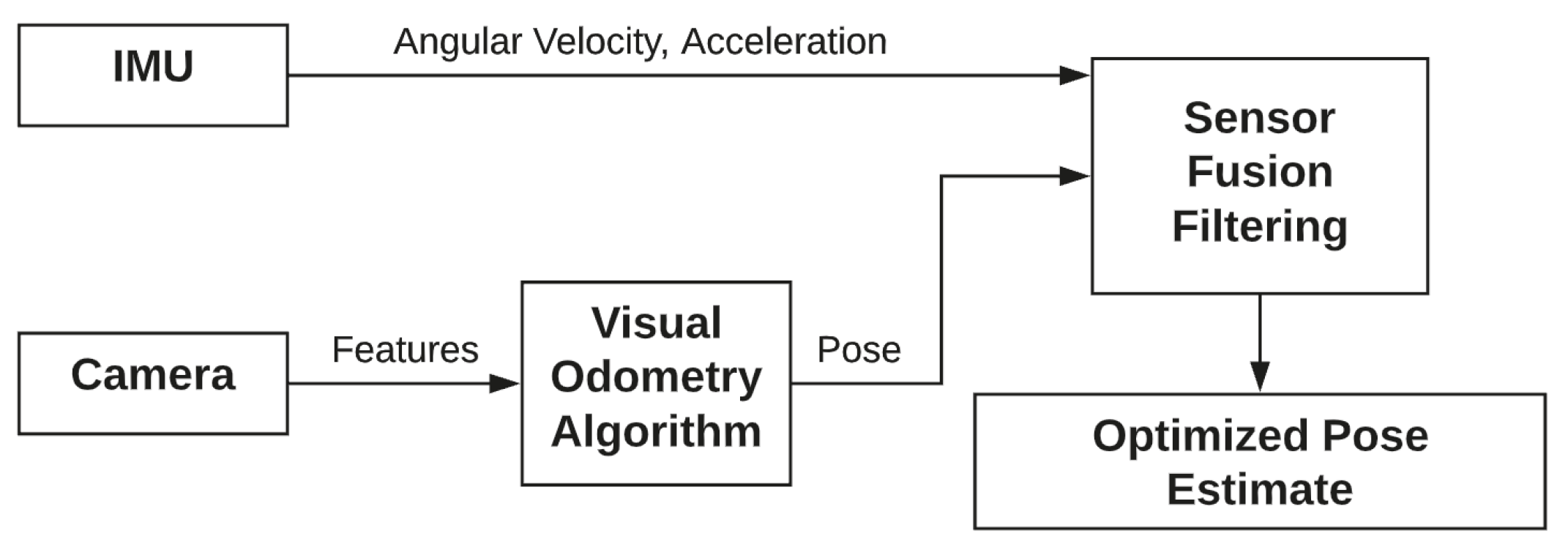
- Loosely coupled: the visual and inertial systems are independent entities. In this case, the fusion is applied through Unscented Kalman filters or Extended Kalman Filters. Although not extremely accurate, this approach favors real-time performance. It also makes easier the integration of information coming from other sensors. The logic is represented in Figure 2.
- (ii)
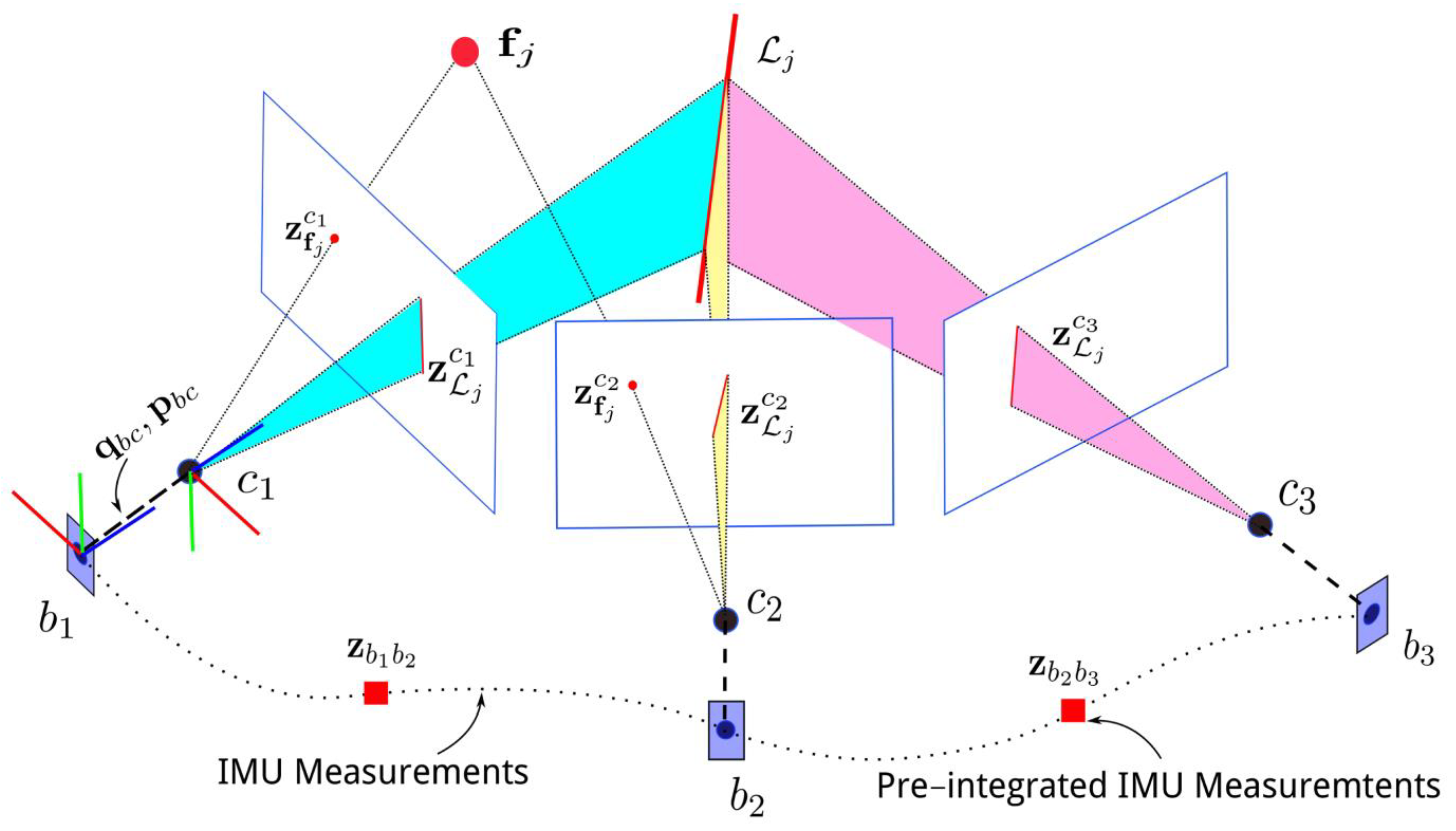
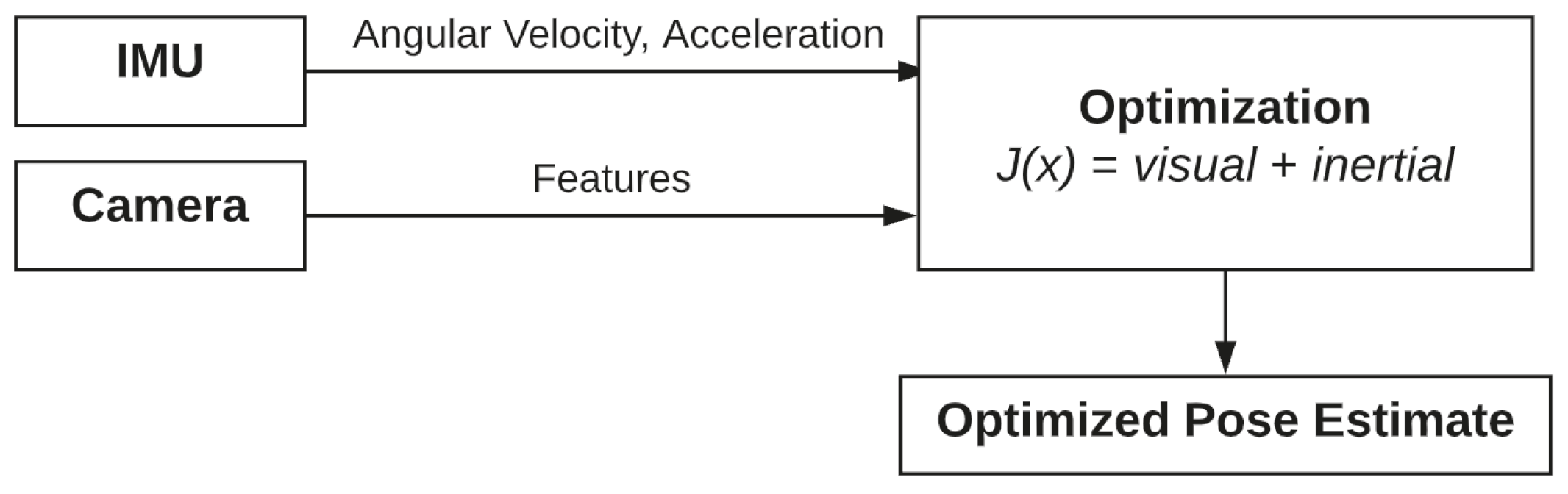
- Tightly coupled: this approach combines visual and inertial parameters in a single optimization problem. This approach involves the data from cameras and the IMU as described in Equation (1). It results more computationally demanding than the loosely coupled approach. As described in [30], the cost function optimization can be written as in Equation (1):where are the weighted reprojection errors of the camera, and are the weighted temporal errors of the IMU. Instead, i represents the camera index, k is the frame index, and j is the image feature index. The approach is shown in Figure 3.
1.1.2. Semi-Direct Visual Odometry for Multi-Camera Systems
2. Methodology
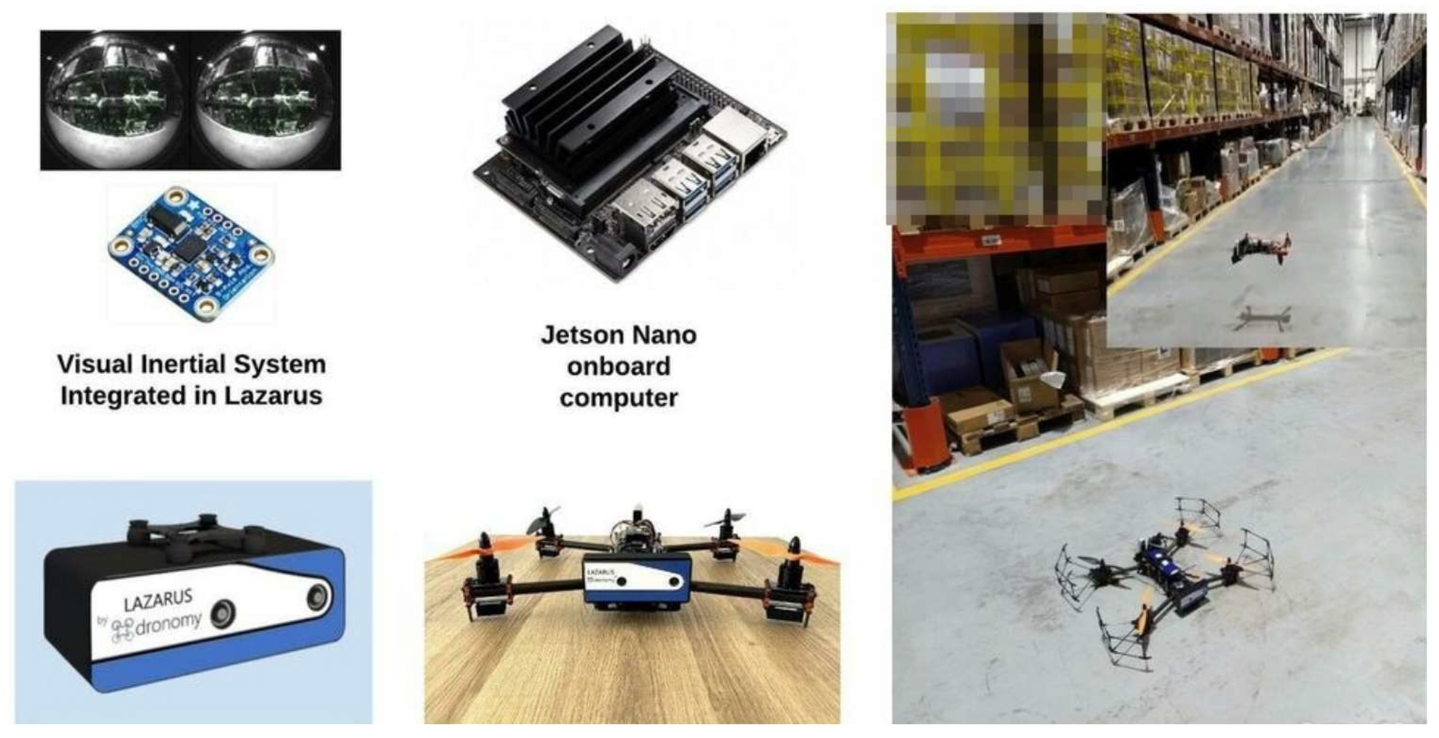
2.1. Hardware Setup
2.2. Sensor Calibration
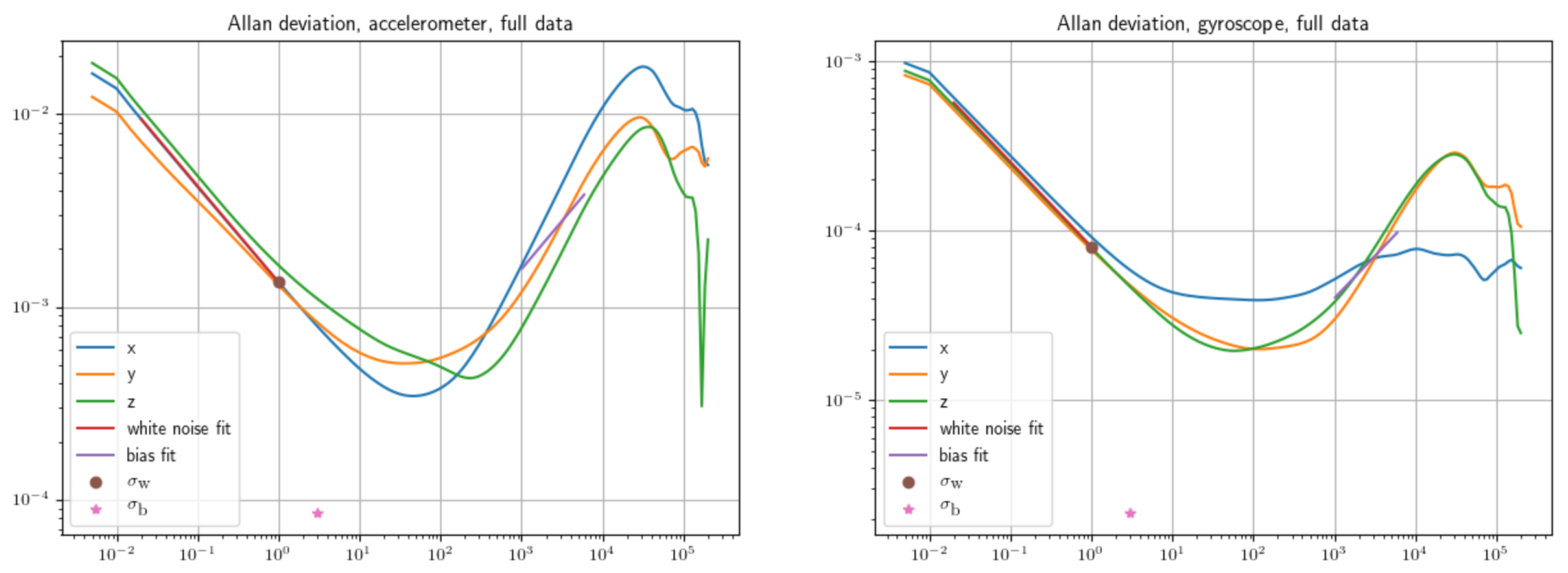
2.2.1. IMU Parameter Extraction
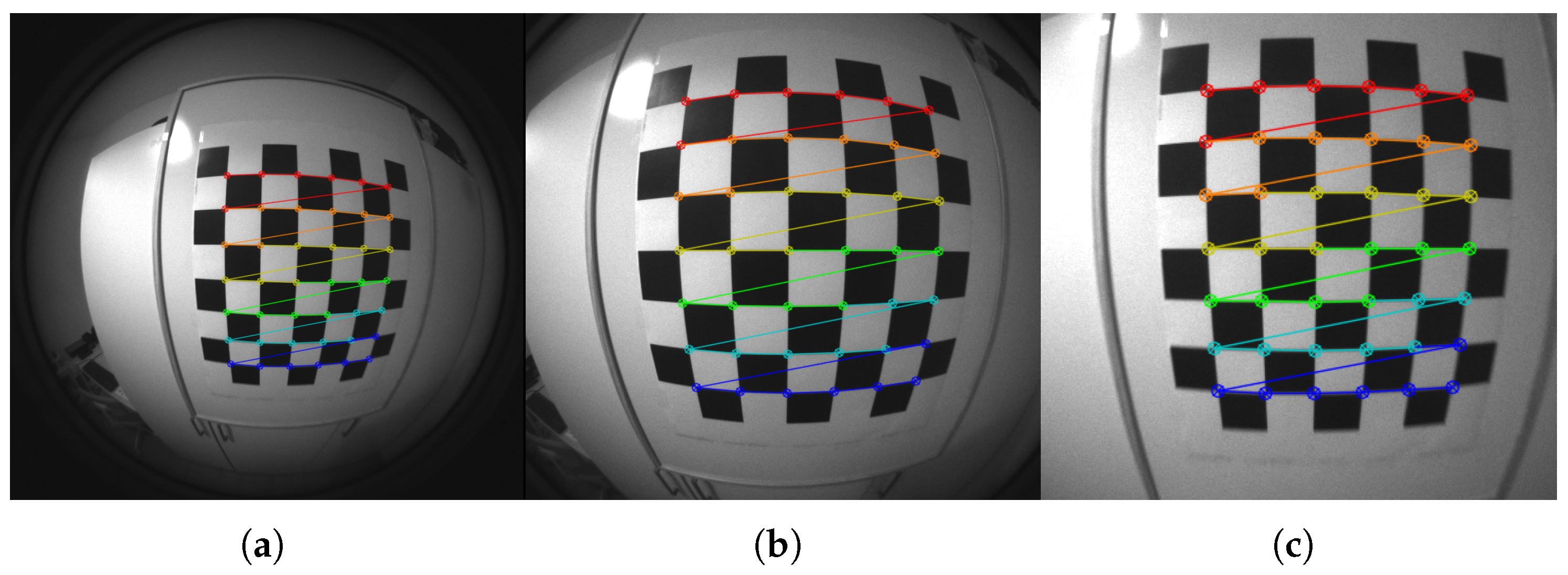
2.2.2. Camera Calibration
2.2.3. Visual-Inertial System Calibration
3. Results and Discussion
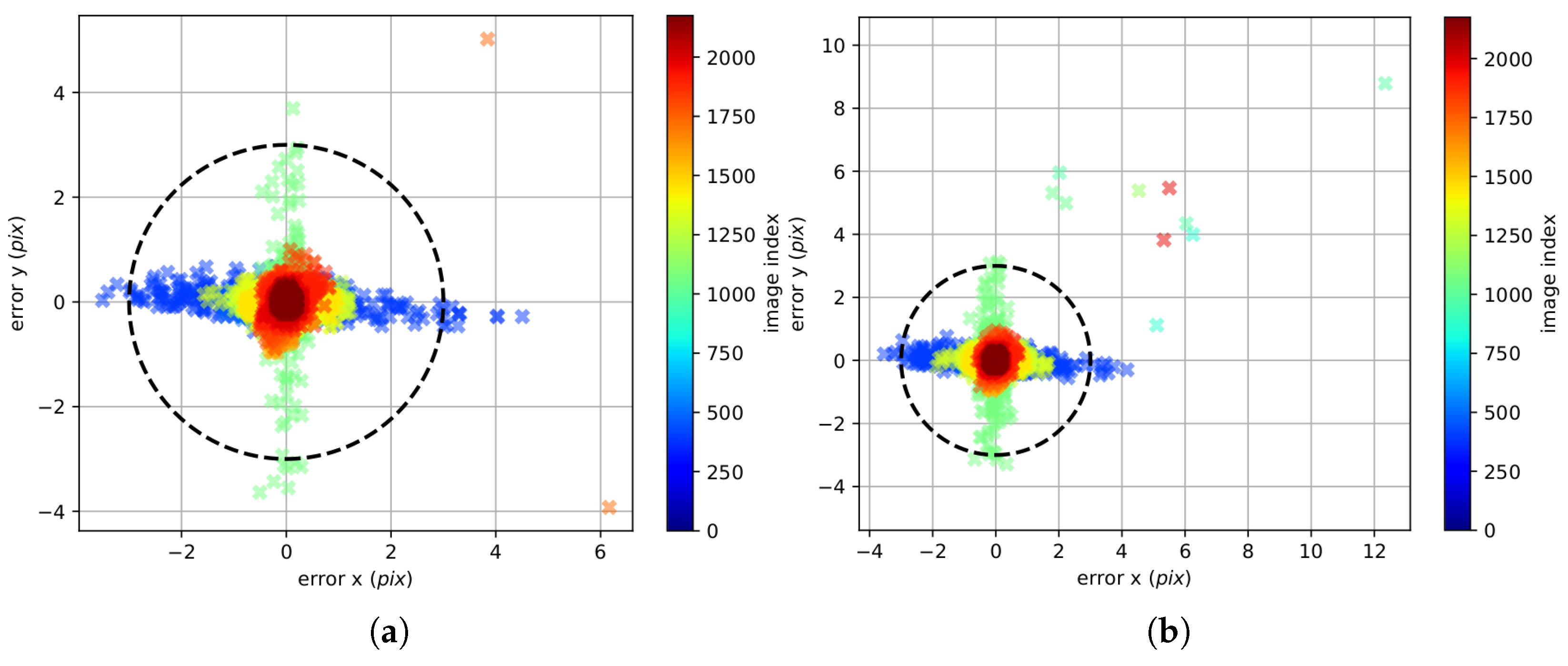
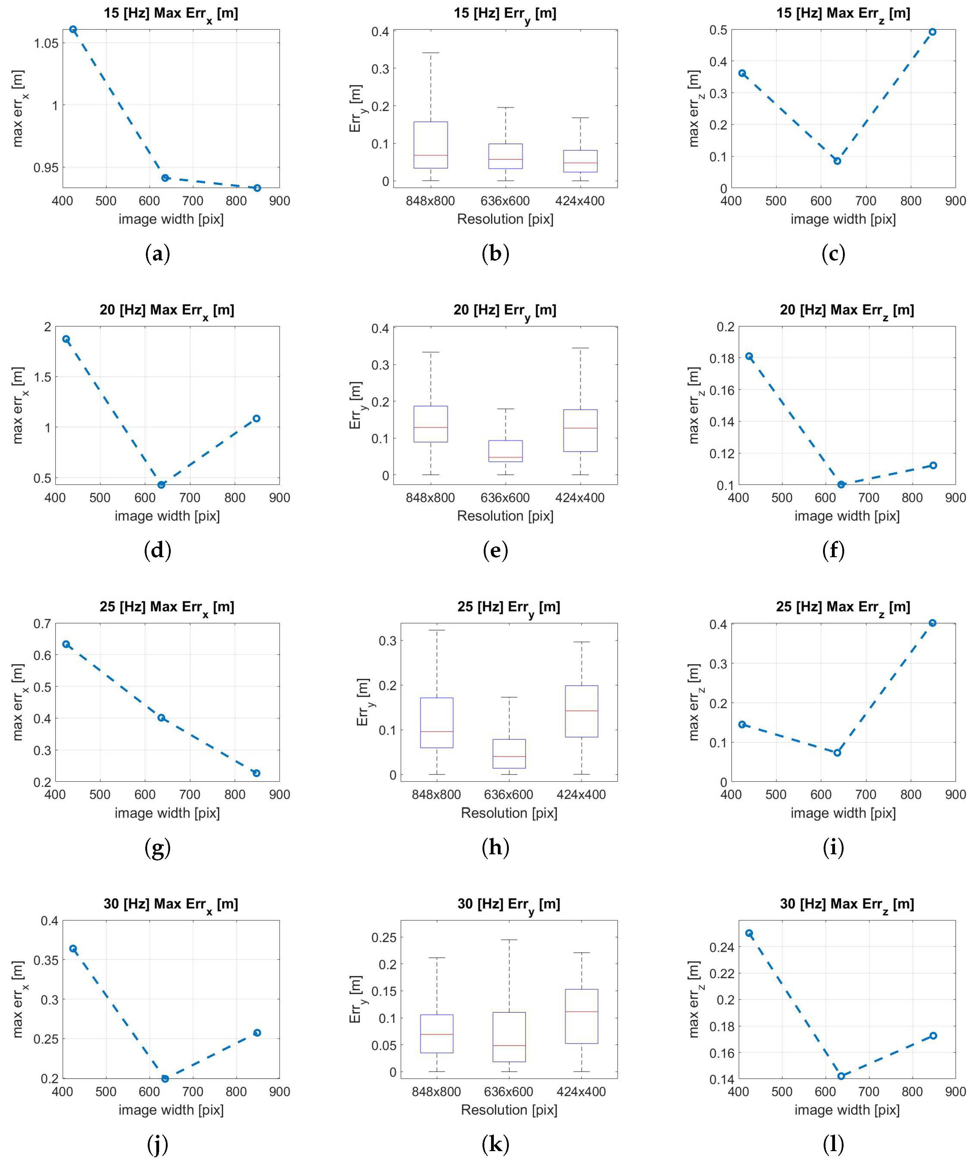
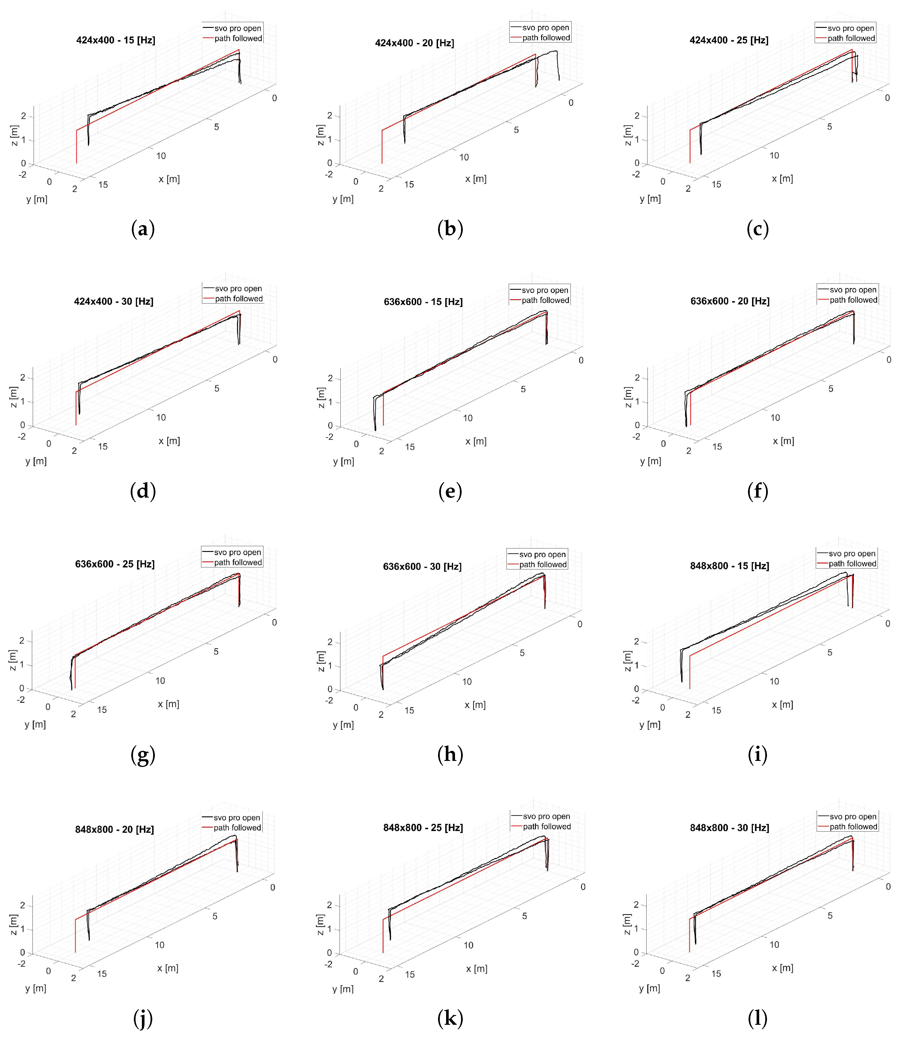
3.1. Translation Error Analysis
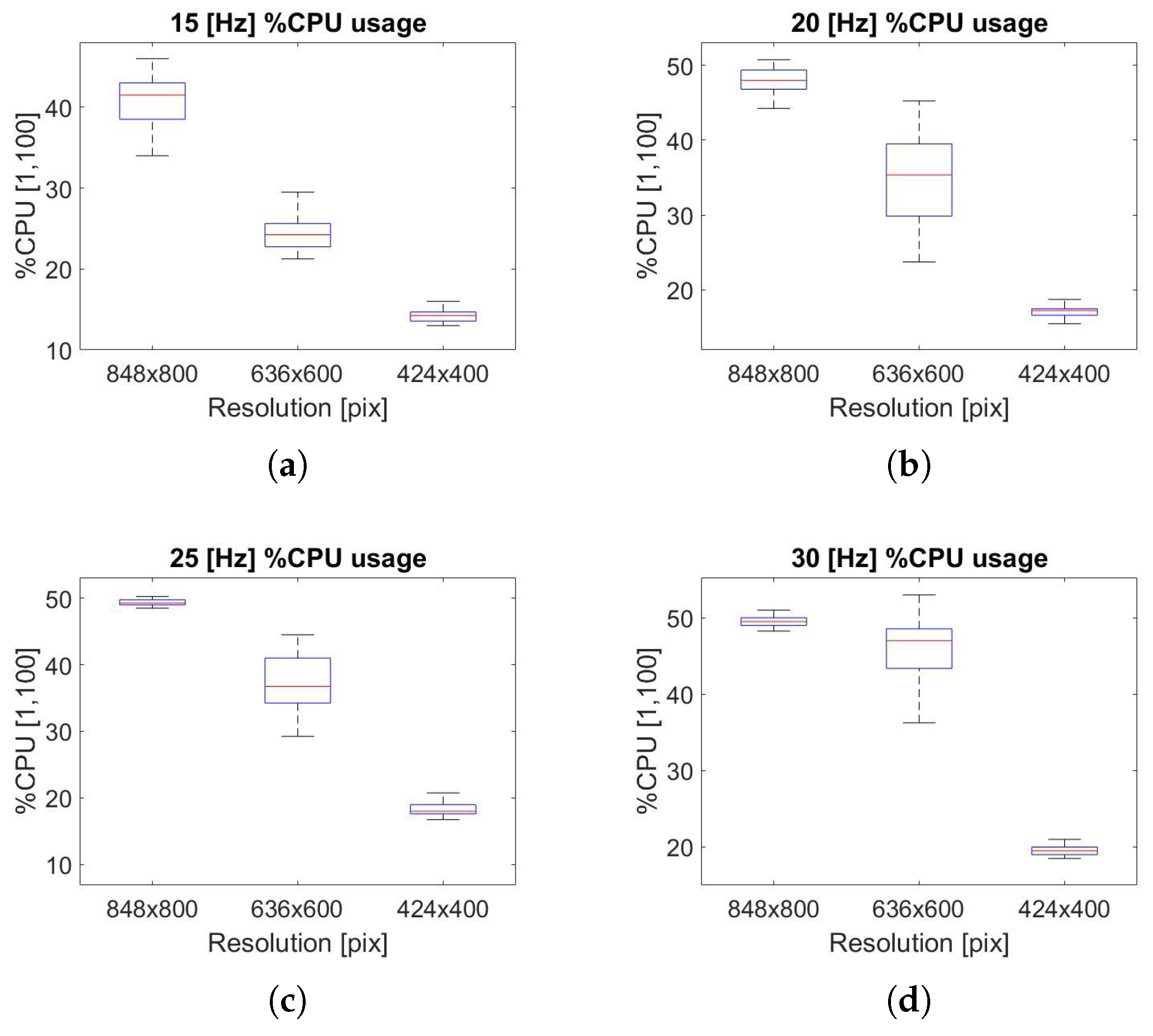
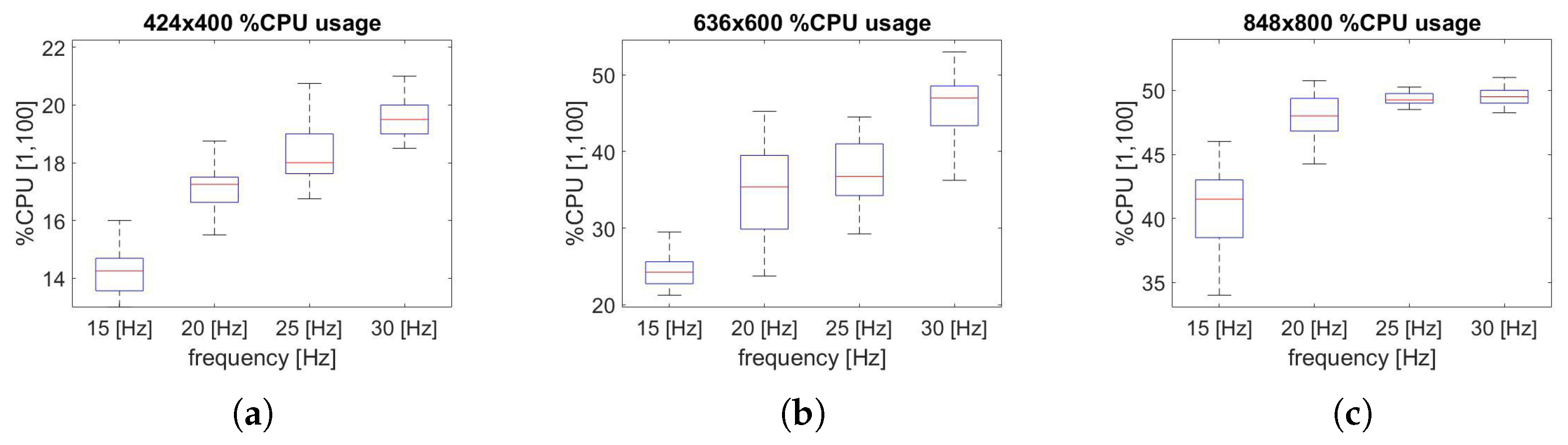
3.2. Computational Cost Analysis
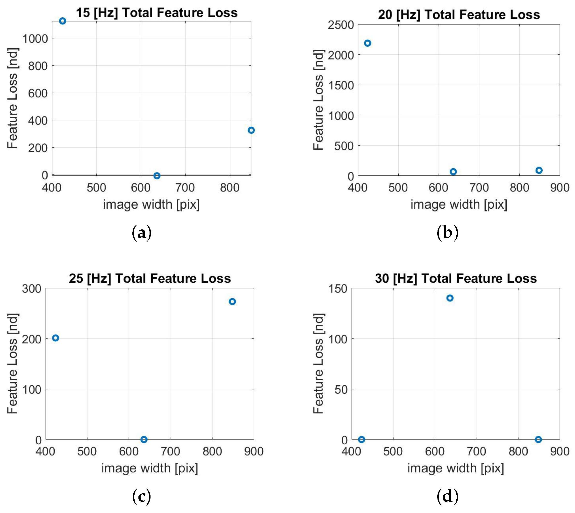
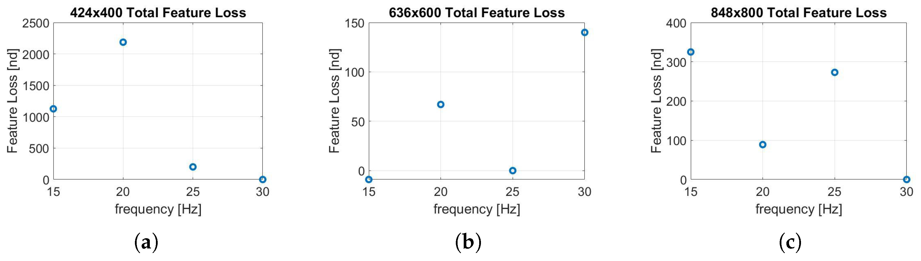
3.3. Feature Loss Analysis
4. Conclusions and Further Developments
Author Contributions
Funding
Institutional Review Board Statement
Informed Consent Statement
Data Availability Statement
Acknowledgments
Conflicts of Interest
Abbreviations
| SVO | Semi-direct Visual Odometry |
| GPS | Global Positioning System |
| UAV | Unmanned Aerial Vehicle |
| CPU | Central Processing Unit |
| ROS | Robot Operating System |
| SLAM | Simultaneous Localization And Mapping |
| RGB | Red Green Blue |
| IMU | Inertial Measurement Unit |
| GPU | Graphics Processing Unit |
| FOV | Field Of View |
| FL | Feature Loss |
References
- Subramanya, K.N.; Rangaswamy, T. Impact of Warehouse Management System in a Supply Chain. Int. J. Comput. Appl. 2012, 54, 14–20. [Google Scholar] [CrossRef]
- Chang, J. Research and Implementation on the Logistics Warehouse Management System. In Proceedings of the 2nd International Conference on Social Science and Technology Education (ICSSTE), Guangzhou, China, 14–15 May 2016. [Google Scholar] [CrossRef]
- Mostafa, N.; Hamdy, W.; Elawady, H. Towards a Smart Warehouse Management System. In Proceedings of the Third North American Conference On Industrial Engineering and Operations (2018), Washington, DC, USA, 27–29 September 2018. [Google Scholar]
- Rey, R.; Corzetto, M.; Cobano, J.A.; Merino, L.; Caballero, F. Human-robot co-working system for warehouse automation. In Proceedings of the 2019 24th IEEE International Conference on Emerging Technologies and Factory Automation (ETFA), Zaragoza, Spain, 10–3 September 2019; pp. 578–585. [Google Scholar] [CrossRef]
- Yuan, Z.; Gong, Y. Improving the Speed Delivery for Robotic Warehouses. In Proceedings of the MIM 2016—8th IFAC Conference on Manufacturing Modelling, Management and Control, Troyes, France, 28–30 June 2016; Volume 49. [Google Scholar]
- De Koster, R.B.M. Automated and Robotic Warehouses: Developments and Research Opportunities. Logist. Transp. 2018, 38, 33–40. [Google Scholar] [CrossRef]
- Panigrahi, P.K.; Bisoy, S.K. Localization strategies for autonomous mobile robots: A review. J. King Saud Univ. Comput. Inf. Sci. 2021, 34, 6019–6039. [Google Scholar] [CrossRef]
- Ubaid, A.; Poon, K.; Altayyari, A.M.; Almazrouei, M.R. A Low-cost Localization System for Warehouse Inventory Management. In Proceedings of the 2019 International Conference on Electrical and Computing Technologies and Applications (ICECTA), Ras Al Khaimah, United Arab Emirates, 19–21 November 2019; pp. 1–5. [Google Scholar]
- Goran, V.; Damjan, M.; Draganjac, I.; Kovacic, Z.; Lista, P. High-accuracy vehicle localization for autonomous warehousing. Robot. Comput. Integr. Manuf. 2016, 42, 1–16. [Google Scholar] [CrossRef]
- Gadd, M.; Newman, P. A framework for infrastructure-free warehouse navigation. In Proceedings of the 2015 IEEE International Conference on Robotics and Automation (ICRA), Seattle, WA, USA, 26–30 May 2015; pp. 3271–3278. [Google Scholar] [CrossRef]
- Oth, L.; Furgale, P.; Kneip, L.; Siegwart, R. Rolling Shutter Camera Calibration. In Proceedings of the 2013 IEEE Conference on Computer Vision and Pattern Recognition, Portland, OR, USA, 23–28 June 2013; pp. 1360–1367. [Google Scholar] [CrossRef]
- Joern, R.; Janosch, N.; Thomas, S.; Timo, H.; Roland, S. Extending kalibr: Calibrating the extrinsics of multiple IMUs and of individual axes. In Proceedings of the IEEE International Conference on Robotics and Automation (ICRA 2016), Stockholm, Sweden, 16–21 May 2016; pp. 4304–4311. [Google Scholar]
- Paul, F.; Joern, R.; Roland, S. Unified Temporal and Spatial Calibration for Multi-Sensor Systems. In Proceedings of the IEEE/RSJ International Conference on Intelligent Robots and Systems (IROS 2013), Tokyo, Japan, 3–7 November 2013. [Google Scholar]
- Paul, F.; Timothy, D.B.; Gabe, S. Continuous-Time Batch Estimation Using Temporal Basis Functions. In Proceedings of the IEEE International Conference on Robotics and Automation (ICRA 2012), Saint Paul, MN, USA, 14–18 May 2012; pp. 2088–2095. [Google Scholar]
- Maye, J.; Furgale, P.; Siegwart, R. Self-supervised Calibration for Robotic Systems. In Proceedings of the IEEE Intelligent Vehicles Symposium (IVS 2013), Gold Coast, Australia, 23–26 June 2013. [Google Scholar]
- Beul, M.; Droeschel, D.; Nieuwenhuisen, M.; Quenzel, J.; Houben, S.; Behnke, S. Fast Autonomous Flight in Warehouses for Inventory Applications. IEEE Robot. Autom. Lett. 2018, 3, 3121–3128. [Google Scholar] [CrossRef]
- Christian, F.; Matia, P.; Davide, S. SVO: Fast Semi-Direct Monocular Visual Odometry; ICRA: Gurgaon, India, 2014. [Google Scholar]
- Christian, F.; Zichao, Z.; Michael, G. Manuel Werlberger, Davide Scaramuzza. SVO: Semi-Direct Visual Odometry for Monocular and Multi-Camera Systems; TRO: Richmond, VA, USA, 2017. [Google Scholar]
- Feng, B.; Zhang, X.; Zhao, H. The Research of Motion Capture Technology Based on Inertial Measurement. In Proceedings of the 2013 IEEE 11th International Conference on Dependable, Autonomic and Secure Computing, Chengdu, China, 21–22 December 2013; pp. 238–243. [Google Scholar] [CrossRef]
- Artyom, M.; Lerke, O.; Prado, M.; Dörstelmann, M.; Menges, A.; Schwieger, V. UAV Guidance with Robotic Total Station for Architectural Fabrication Processes. In ICD/ITKE Research Pavilion 2016-17 Aerial Construction—Flying Robots for Architectural Fabrication; Wißner: Augsburg, Germany, 2017. [Google Scholar]
- Hu, X.; Luo, Z.; Jiang, W. AGV Localization System Based on Ultra-Wideband and Vision Guidance. Electronics 2020, 9, 448. [Google Scholar] [CrossRef]
- Carlos, C.; Richard, E.; Gomez, J.J.; Montiel, J.M.M.; Tardós, J.D. ORB-SLAM3: An Accurate Open-Source Library for Visual, Visual-Inertial and Multi-Map SLAM. arXiv 2020, arXiv:2007.11898. [Google Scholar]
- Qin, T.; Li, P.; Shen, S. VINS-Mono: A Robust and Versatile Monocular Visual-Inertial State Estimator. IEEE Trans. Robot. 2018, 34, 1004–1020. [Google Scholar] [CrossRef]
- Sun, K.; Mohta, K.; Pfrommer, B.; Watterson, M.; Liu, S.; Mulgaonkar, Y.; Taylor, C.J.; Kumar, V. Robust Stereo Visual Inertial Odometry for Fast Autonomous Flight. IEEE Robot. Autom. Lett. 2017. [Google Scholar] [CrossRef]
- Bloesch, M.; Burri, M.; Omari, S.; Hutter, M.; Siegwart, R. Iterated extended Kalman filter.based visual-inertial odometry using direct photometric feedback. Int. J. Robot. Res. 2017, 36, 1053–1072. [Google Scholar] [CrossRef]
- Scaramuzza, D.; Fraundorfer, F. Visual Odometry: Part I—The First 30 Years and Fundamentals. IEEE Robot. Automat. Mag. 2011, 18, 80–92 (cit. on pp. 11–13, 16, 30–33). [Google Scholar] [CrossRef]
- Mueggler, E.; Gallego, G.; Rebecq, H.; Scaramuzza, D. Continuous-Time Visual-Inertial Odometry for Event Cameras. IEEE Trans. Robot. 2018, 34, 1425–1440. [Google Scholar] [CrossRef]
- He, Y.; Zhao, J.; Guo, Y.; He, W.; Yuan, K. PL-VIO: Tightly-Coupled Monocular Visual–Inertial Odometry Using Point and Line Features. Sensors 2018, 18, 1159. [Google Scholar] [CrossRef] [PubMed]
- Burusa, A.K. Visual-Inertial Odometry for Autonomous Ground Vehicles. In Degree Project In Computer Science And Engineering, Stockholm; DiVA: Luleå, Sweden, 2017. [Google Scholar]
- Leutenegger, S.; Lynen, S.; Bosse, M.; Siegwart, R.; Furgale, P. Keyframe-based visual–inertial odometry using nonlinear optimization. Int. J. Robot. Res. 2015, 34, 314–334. [Google Scholar] [CrossRef]
- Suriano, F. Study of SLAM State of Art Techniques for UAVs Navigation in Critical Environments. In Degree Project in Aerospace Engineering, 16 Credits; Politecnico di Torino: Turin, Italy, 2021. [Google Scholar]
- Barfoot, T.D. State Estimation for Robotics—A Matrix Lie Group Approach; Cambridge University Press: Cambridge, UK, 2015. [Google Scholar]
- Valladares, S.; Toscano, M.; Tufino, R.; Morillo, P.; Vallejo, D. Performance Evaluation of the Nvidia Jetson Nano Through a Real-Time Machine Learning Application. Int. Conf. Intell. Hum. Syst. Integr. 2021, 1322, 343–349. [Google Scholar] [CrossRef]
- Woodman, O.J. An Introduction to Inertial Navigation (Research Report696); University of Cambridge: Cambridge, UK, 2007. [Google Scholar]
- Ciarán, H.; Robert, M.; Patrick, D.; Martin, G.; Edward, J. Equidistant fish-eye perspective with application in distortion centre estimation. Image Vis. Comput. 2010, 28, 538–551. [Google Scholar] [CrossRef]
- Shah, S.; Aggarwal, J.K. Intrinsic parameter calibration procedure for a (high-distortion) fish-eye lens camera with distortion model and accuracy estimation. Pattern Recognit. 1996, 29, 1775–1788. [Google Scholar] [CrossRef]
- Hu, G.; Zhou, Z.; Cao, J.; Huang, H. Nonlinear calibration optimization based on the Levenberg-Marquardt algorithm. IET Image Process. 2019, 14, 1402–1414. [Google Scholar] [CrossRef]


| Parameter | Symbol | BNI055 | Unit |
|---|---|---|---|
| Gyroscope “white noise” | 0.0018491 | rad (s | |
| Accelerometer “white noise” | 0.01094 | m (s2 | |
| Gyroscope “bias instability” | rad | ||
| Accelerometer “bias instability” | 0.00058973 | m |
| Param | ||||||
|---|---|---|---|---|---|---|
| 285.3568 | 285.3568 | 285.7695 | 285.5315 | 285.5315 | 285.3433 | |
| 285.4461 | 285.4461 | 285.6246 | 285.5397 | 285.5397 | 285.1813 | |
| 419.0777 | 310.2573 | 207.0993 | 414.3119 | 305.4019 | 202.1401 | |
| 399.5762 | 297.1926 | 200.8910 | 396.4943 | 294.4193 | 196.9490 | |
| −0.005900 | −0.005900 | −0.005900 | −0.006894 | −0.006894 | −0.006894 | |
| 0.04159 | 0.04160 | 0.04160 | 0.04397 | 0.04397 | 0.04397 | |
| −0.03861 | −0.03861 | −0.03861 | −0.04040 | −0.04040 | −0.04040 | |
| 0.006450 | 0.006451 | 0.006451 | 0.006843 | 0.006843 | 0.006843 |
| Freq (Hz) | Mean (% CPU) | Max (% CPU) | Min (% CPU) |
|---|---|---|---|
| 15 | 13.968 | 16 | 5.5 |
| 20 | 16.578 | 19.25 | 4 |
| 25 | 18.148 | 21.5 | 9 |
| 30 | 19.056 | 24.25 | 7.5 |
| Freq (Hz) | Mean (% CPU) | Max (% CPU) | Min (% CPU) |
|---|---|---|---|
| 15 | 24.543 | 30.5 | 21.25 |
| 20 | 34.993 | 45.25 | 23.75 |
| 25 | 37.298 | 44.5 | 29.25 |
| 30 | 45.31 | 53 | 30.5 |
| Freq (Hz) | Mean (% CPU) | Max (% CPU) | Min (% CPU) |
|---|---|---|---|
| 15 | 40.658 | 46 | 34 |
| 20 | 48.048 | 50.75 | 44.25 |
| 25 | 49.467 | 51 | 48.5 |
| 30 | 49.637 | 53 | 48.25 |
Publisher’s Note: MDPI stays neutral with regard to jurisdictional claims in published maps and institutional affiliations. |
© 2022 by the authors. Licensee MDPI, Basel, Switzerland. This article is an open access article distributed under the terms and conditions of the Creative Commons Attribution (CC BY) license (https://creativecommons.org/licenses/by/4.0/).
Share and Cite
Godio, S.; Carrio, A.; Guglieri, G.; Dovis, F. Resolution and Frequency Effects on UAVs Semi-Direct Visual-Inertial Odometry (SVO) for Warehouse Logistics. Sensors 2022, 22, 9911. https://doi.org/10.3390/s22249911
Godio S, Carrio A, Guglieri G, Dovis F. Resolution and Frequency Effects on UAVs Semi-Direct Visual-Inertial Odometry (SVO) for Warehouse Logistics. Sensors. 2022; 22(24):9911. https://doi.org/10.3390/s22249911
Chicago/Turabian StyleGodio, Simone, Adrian Carrio, Giorgio Guglieri, and Fabio Dovis. 2022. "Resolution and Frequency Effects on UAVs Semi-Direct Visual-Inertial Odometry (SVO) for Warehouse Logistics" Sensors 22, no. 24: 9911. https://doi.org/10.3390/s22249911
APA StyleGodio, S., Carrio, A., Guglieri, G., & Dovis, F. (2022). Resolution and Frequency Effects on UAVs Semi-Direct Visual-Inertial Odometry (SVO) for Warehouse Logistics. Sensors, 22(24), 9911. https://doi.org/10.3390/s22249911