The proposed DWL framework consists of the following stages (
Figure 1),
A. Pre-processing,
B. Motion-artifact Detection,
C. Motion-artifact Frequency Components Identification,
D. Denoising, and
E. Heart Rate Estimation. The inputs to the system are raw green and IR PPG signals measured using the dual-wavelength PPG wrist-unit sensor (described in
Section 2.1). The output is an HR estimate,
at time step
l (the initial time step is
). We refer to the average of the latest
Z estimates of the heart rate as
, namely
Figure 3 is a block diagram of the DWL method. The system produced a new estimate of HR at every time step (
at time step
l). The time between two subsequent windows in our study was 2 s. In addition, the system produces three
search ranges. They are; the “narrow search range”,
; the “medium search range”,
; and the “wide search range”,
. Ranges
and
, which are used in the motion-artifact frequency components identification process of
Section 2.3.3, are centered at
. The range
, which is used in the heart rate estimation process of
Section 2.3.5, is centered at
, the average of the 6 previous heart rate estimates. The ranges satisfy
. Moreover,
(for details on how we calculated
and
, see Equations (
A2) and (
A4) in
Appendix A, respectively). Lastly, we calculate a short-term 3-point-average heart rate,
, that we provide to the users and employ in
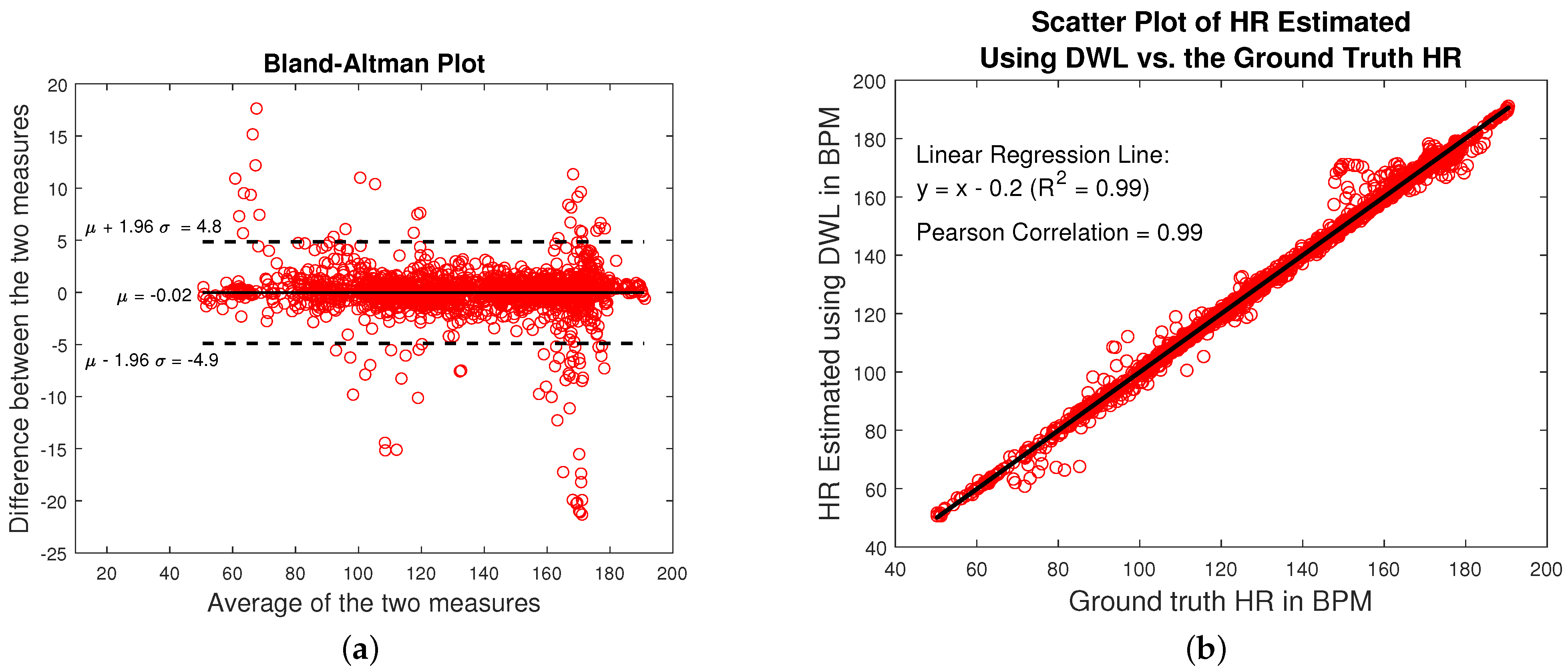
Section 3.2 for assessing the performance of DWL.
Figure 4 is an illustration of a typical IR PPG spectrum. The magenta dashed line in
Figure 4a is the heart rate estimated at time step
l,
. The black dotted line in
Figure 4b is the average of the 6 previous heart rate estimates at time step
l,
. In this example,
is 1.5 Hz and
is 1.45 Hz. Additionally, we present in
Figure 4 the “wide search range”,
, as a green dashed rectangle, the “medium search range”,
, as a red dashed rectangle, and the “narrow search range”,
, as a blue dashed rectangle.
2.3.2. Motion-Artifact Detection
Motion artifact detection is used to determine whether the PPG signals are contaminated by motion noise (if they are not, we can bypass unnecessary noise suppression operations). The PPG signals go through the following three (3) local detectors to determine if appreciable levels of noise motion are present (block B of
Figure 3):
Local Detector 1 ()—Number of Peaks: The number of dominant peaks (whose magnitude exceeds 30% of the maximum peak for this example) in the frequency spectrum of the green PPG signal, denoted , is calculated. If exceeds two (2), indicates that the signal is contaminated with motion noise. If is 1 or 2, then we conclude that no appreciable motion noise is present, since the frequency of the heart rate and sometimes its second harmonic component are typically observed in the spectrum of a clean PPG signal.
Local Detector 2 (
)—Power of Green Signal: The power of the green PPG signal calculated at the beginning of the experiment (when the participant is at rest) is considered the reference power, denoted
. At each time step
l, the power of the green PPG,
, is calculated and compared to the reference power
. If
is more than
,
indicates that the green PPG signal is contaminated with motion noise. The amplitude of the PPG signal might change over time [
24]. Therefore, the reference power
is updated whenever no motion is detected in the system for five (5) consecutive time steps (global detector
return ‘1’). In this case, the updated value of
is set to the power of the green PPG signal calculated at the current time step,
l. In this study, we used
.
Local Detector 3 ()—Pearson Correlation between Green and IR PPG Signals: The correlation between the green and IR PPG signals is also used to assess noise contamination in the green signal. If the correlation between the green and IR PPG signals, , is below a certain threshold (we used 0.8), then will decide that the green PPG signal is contaminated with motion noise.
Global Detector—Noise Detector: The decisions of the three local detectors are fed into a global detector that will decide whether the signal is noise contaminated. The global detector is shown as:
where “∨” represents the OR logic operator.
2.3.3. Motion-Artifact Frequency Components Identification
If motion artifacts are detected in the normalized green PPG signal, we use the normalized IR signal to build the motion noise component set
(block C of
Figure 3).
can be written as
where
is the
discrete noise frequency component and
is the number of elements in the set
. The set
, which contains all the noise frequency components that we aim to remove from the normalized green PPG signal, is obtained using the following five (5) steps in sequence. The first three steps capture noise with relatively high intensity, usually harmonically related frequency pairs that contaminate the PPG signals. The last two steps compare the IR and green signal spectra to discover additional noise components of reduced-intensity presence in the IR spectrum.
Step 1—Identification of dominant frequency components. First, we capture the dominant frequency components in the spectrum of the normalized IR PPG signal. Those are the frequencies (between 0.5 and 4 Hz) whose magnitude exceeds 50% of the highest peak in the IR PPG spectrum.
Figure 5, which is an image that was created for illustration purposes, depicts how we capture dominant peaks from a typical IR signal. In this scenario, the highest peak (which actually corresponds to the participant’s HR) is
. Two other dominant peaks are shown as red circles (
and
). Typically, the peaks captured in step 1 include the frequency of the participant’s HR, as well as the frequencies of dominant noise components. We add all of them (
,
, and
in our example) to
with the understanding that one of them may correspond to the participant’s HR and may therefore need to be removed from
later.
Step 2—Identification of harmonic frequency components. Noise components created by repetitive motion (e.g., when the participant is walking or running) typically occur in harmonically related pairs [
25]. It is possible, however, that the PPG signal contains pairs of harmonically related noise components whose magnitude is smaller than the 50% threshold used in step 1 to identify dominant frequencies. Step 2 is used to capture pairs of fundamental frequencies and their second harmonics present in the spectrum of the normalized IR PPG signal. Here, we look at all peaks whose magnitudes are above 30% of the highest peak in the IR PPG spectrum. For each such peak, we search for a harmonic at double its frequency. If a pair of harmonically related frequencies is thus discovered, its component(s) that were not flagged in step 1 are added to the noise frequency set
. Again,
may still contain at this stage a component that corresponds to the participant’s true HR.
Figure 6 uses the same spectrum shown in
Figure 5 to illustrate how a pair of harmonically related components (
,
) was discovered. Of this pair,
was known to us already from step 1 (it is the same as
in
Figure 5), and
, discovered by step 2, is added to
. So now,
.
Step 3—Removal of the heart rate from noise set. As mentioned in our setting in
Section 2.3, our system creates a new estimate of the heart rate,
at every time step
l. A new time step starts every 2 s when
l is incremented by 1. Moreover, in step
we calculate
(the “wide search range”) which is where we search for
.
Next, frequency components in which we captured during steps 1 and 2, and are close to the heart rate estimated at time step l () are removed from , as we suspect they do not represent noise but rather represent the participant’s HR. To be precise, at time step , we remove from all the noise components in the “medium search range” .
Figure 7 continues the examples of
Figure 5 and
Figure 6 to illustrate step 3. In
Figure 7a,b, we show the estimate of the participant’s HR at time step
l, denoted
. We also show
, the “medium search range”,
, from which we remove dominant frequencies deposited earlier into
. The red squares in
Figure 7a represent the frequency components that we obtained from steps 1 and 2 all of which are currently in
. We now discard the frequency around 1.2 Hz (labeled
) since it falls in
, the “medium search range” (region represented by a red dashed rectangle in
Figure 7).
Figure 7b shows (in red squares) the noise frequency components that are left in the noise set
.
no longer contains the participant’s HR.
The next two steps seek additional noise components, often attributed to repetitive movements by the participant, through comparison of the IR and green spectra.
Step 4: Step 4 focuses on instances where the noise set , after step 3, has only one noise component, . In this case, we look at the green spectrum. If we find a component at half () or twice () in the green spectrum, we add this component to . The only exception is if the component we seek to add falls into the narrow search range, , around , ; in this case, we refrain from adding it to set .
Step 5: This step addresses spectra that are dominated by vigorous limb swinging by the participant, which may cause displacement of the sensor. In this scenario, the green PPG signal is typically dominated by two high intensity harmonically related noise frequencies which may dwarf the component at the heart rate frequency. If these frequency components are not already placed in after steps 1–3, they are added to at this step. This step is automatically triggered when all the following conditions are met, namely; (a) the IR spectrum contains only one significant frequency component that dominates the spectrum; (b) the green spectrum contains only one pair of significant harmonically related frequencies; and (c) the dominant frequency component present in the IR spectrum matches one of the harmonically related frequencies discovered in the green spectrum.
Figure 8 is a real-life example that illustrates this scenario (signals were collected from participant 10 in our experiment, around time 136 s). We show the spectrum of participant 10’s IR signal in
Figure 8a and green signal in
Figure 8b. We show in magenta the heart rate estimate at time step
l,
. The green signal captures the high-intensity harmonically related frequency pairs
and
of
Figure 8b. The IR spectrum (
Figure 8a) is dominated by the frequency
that is equal to frequency
from the green spectrum, but does not capture a noise component at
. Here, frequencies
and
are put into
.
At the end of this stage, the set will contain elements that correspond to the noise frequencies we wish to remove from the normalized green PPG signal.
2.3.4. Denoising
Adaptive Noise Cancellation (ANC) filters are often employed to eliminate in-band motion artifacts [
26,
27]. In-band noise in our case occurs when the spectra of motion artifacts overlap significantly with that of the PPG signal [
28]. An ANC filter for our environment would use as inputs (1) a noise contaminated signal, and (2) a noise reference signal. The ANC filter seeks to eliminate the noise components (measured by the reference signal) from the input noise contaminated signal and provide a noise-free version of the input signal.
Motivated by the architecture in [
29], we employ a Cascading Adaptive Noise Cancellation (C-ANC) architecture to remove all the elements of the set
(developed in
Section 2.3.3) from the green PPG signal,
one element at the time. The block diagram of the proposed C-ANC is shown in
Figure 9. We show the frequency spectrum of the input signal in
Figure 9 (spectrum A). This is the green signal collected from participant 3 around time 66 s. The spectrum contains three noise frequency components that we wish to eliminate from the signal. The signal collected at the output of the C-ANC (spectrum D in
Figure 9) does not contain any of the noise components; only the HR frequency component remained in the spectrum.
A total of
C-ANC were used to remove the noise components of
from the green PPG signal. At the
stage (
), the noise reference signal is a pure sinusoid of frequency
. For instance, the first ANC filter block shown in
Figure 9 removes the first noise frequency component
from the normalized green PPG signal (see spectrum B of
Figure 9). The output of the first block is denoted
.
is fed to the next block where the second noise frequency component
is removed (see spectrum C of
Figure 9). The process is repeated until all noise components are removed from the normalized green PPG signal. The final output,
, is a noise-free version of the green PPG signal. In the proposed method, the QR-decomposition-based least-squares lattice (QRD-LSL) adaptive filter algorithm was used to remove noise components from the green PPG signal [
30]. The method incorporates the desirable features of recursive least-square estimation (fast convergence rate), QR-decomposition (numerical stability), and lattice structure (computational efficiency) [
12]. The implementation of the QRD-LSL filter in our study used the built-in MATLAB function “
AdaptiveLatticeFilter” [
31] with 10 filter taps and forgetting factor of 0.99.
2.3.5. Heart Rate Estimation
In this stage (see block E of
Figure 3), the green PPG signal is used to compute an HR value. If no noise was detected in the green PPG (
), then the normalized green PPG is used for heart rate calculation. When noise was detected in the green PPG signal, a HR value is obtained from the denoised green signal (obtained at the output of block D in
Figure 3, also shown in
Figure 9). The “Heart Rate Estimation” stage comprises two steps, namely, “Initialization” and “Heart Rate Calculation”.
Initialization (block E1 of
Figure 3). This is a process of capturing a baseline HR at rest. In our experiment, it was a one-minute phase during which participants were asked to remain steady in order to capture noise-free green and IR PPG signals. To calculate the initial HR estimate,
at time step
, we used the frequency spectrum of the normalized green PPG signal.
corresponds to the highest peak within the initial search range 0.5 to 3 Hz (which corresponds to 30 to 180 BPM).
Heart Rate Calculation (block E2 of
Figure 3). At time step
, the heart rate calculation method we propose employs the following variables in order to generate an HR estimate,
:
- 1.
The heart rate estimated from the previous time step l, .
- 2.
A heart rate candidate which is obtained from the spectrum of the green PPG signal.
- 3.
A heart rate prediction,
which is obtained from the long-term (LT) trend of the past six (6) HR estimates. The LT trend is obtained using STL, the Seasonal-Trend decomposition using LOESS (locally estimated scatterplot smoothing) [
32]. In this study, we used the MATLAB implementation,
trenddecomp.
First, we seek to find an HR candidate, , within the wide search range , which corresponds to the highest peak in the green spectrum (). If is available, we calculate , which is the absolute difference between and (in Hz) at time step . We distinguish between four (4) cases.
Case 1. If a peak is found inand(“no noise”) OR If a peak is found inand(“noise is present”) andHz.
In this case,, corresponds to the highest peak in the green spectrum, within the wide search range (
). The estimated heart rate, is calculated as Case 2. If a peak is found inandandHz.
In this case, we follow the procedure recommended in [7] to consider at most three dominant peaks in the green spectrum, whose magnitude exceed 50% of the maximum peak. Here,is obtained by averaging all the peaks that we considered. The estimated heart rate,is calculated aswhereis a constant we set to 0.9. Case 3. If no peak is found in.
In this case, we extend the wide search range,. The extended wide search range is (
in this study). We seek to find at most three dominant peaks within the extended wide search range, (the range ). If we find at least one peak, we consider at most three dominant peaks, whose magnitude exceed 50% of the maximum peak. is obtained by averaging all the peaks that we considered. The estimated heart rate, is calculated aswhere is a constant we set to 0.9. Case 4. If no peak is found inor in.
In this case,is calculated as The heart rate calculation process we used requires the availability of the previous six HR estimates in order to generate an HR prediction,
at time step
. Therefore, from time steps
to
, the HR estimates
through
corresponds to the highest peak in the green spectrum, within the wide search range
(
). If no such peak is detected, we increment
by 0.02 Hz (or 1.2 BPM) and we search again for a peak. This process repeats until a peak is found.
is the average of all the previously calculated HR estimates (see Equation (
3)).


 ,
, 


