Abstract
This paper proposes the procedure for minimising the dynamic error in the time and frequency domains, based on the example of a second-order sensor. Our procedure includes three main steps: modelling of the sensors using the Monte Carlo (MC) method; determination of the maximum value of the dynamic error using the integral-square criterion (ISC); and optimisation of the parameters of the sensor model by minimising the ISC. The uncertainties associated with the modelling procedure and the MC method are also considered. The mathematical formulae necessary for implementation in a given programming language (MathCad, MATLAB, C, etc.) are presented in detail. The proposed procedure was implemented in the frequency domain, using MathCad 15, and applied to the example of the Althen 731-207 accelerometer. Validation of the proposed procedure was carried out using a digital signal processor of type TMS320C6713. The proposed procedure can increase the accuracy of the signal processing obtained at the output of sensors applied to a wide range of measurements.
1. Introduction
The min–max method has been applied to minimise the dynamic error of a wide class of measurement systems [1,2] and can be used for the optimisation of both single- and multi-criteria systems [3]. Application of the min–max procedure yields satisfactory results by first considering the upper bound on the dynamic error (UBDE) (the max stage of the min–max algorithm) [4,5,6], and then by applying a selected procedure for minimising this criterion (the min stage) [7,8]. Two basic quality criteria are typically used for the dynamic measurement: i.e., the integral-square criterion (ISC) [7,9] and the absolute error criterion [5].
The UBDE is the maximum value of the dynamic error and depends on both the dynamic properties of the sensor and the shape of the input signal [7]. It is determined by computer simulation based on the mathematical model of the sensor [10,11,12] and the test signal used at the input. The shapes most often considered are linearly and parabolically increasing signals [13], a random Gaussian process [14], or a specially defined function of time [15]. However, such signals do not reflect the real inputs to the sensors.
A mapping of the realistic shapes of the input signals can be obtained when test signals with constraints are used [7,16]; however, this approach requires the use of special computational procedures, including tools such as algorithms to solve the system of convolutional equations (after their optimal number has been determined) [17], procedures based on the genetic method [17,18], and procedures using the fixed-point algorithm (FPA) [9,19]. However, the influence of the uncertainty [20,21] associated with the sensor modelling on the value of the dynamic error is not considered in these procedures.
At the min stage, there are many possibilities for the selection of the dedicated algorithm. Procedures based on the genetic method and the Levenberg-Marquardt algorithm [17,18] have been developed for the UBDE step. However, the influence of the modelling uncertainty on the obtained result, and the propagation of uncertainties by the corresponding computational procedure, have not been considered [21,22].
In view of the limitations of the min–max procedure, we propose the procedure based on the FPA and the Monte Carlo (MC) method [23,24,25,26,27]. Although our procedure involves minimising the dynamic error for second-order sensors [28], it can easily be extended to the sensors with dynamics of different orders. We chose to focus on second-order sensors in this paper because a significant proportion of real sensors are defined by this dynamic order, such as vibration and pressure sensors [28,29,30,31,32], and the mechanical construction of a wide variety of other measurement instruments [33]. The proposed procedure can be applied in both the time and frequency domains [34,35,36], which are used in practical implementations of procedures intended for sensor modelling. The solutions proposed in this study consists of three main steps:
- Modelling of the sensors using the MC method. In addition to the parameters of the sensor mathematical model under consideration, the uncertainties associated with these parameters are also considered [37,38,39]. Pseudo-random number generators with normal and uniform distributions are used to implement the MC method [40,41,42], which has an advantage over other alternative procedures as it can be implemented in both the time and frequency domains.
- Determination of the UBDE for the ISC by imposing magnitude and time constraints on the input test signal [7,17]. FPA, which is highly computationally effective, is used here to determine the UBDE [9,19].
- Optimisation of the sensor parameters using the MC method. The min–max procedure proposed in this paper allows us to select the parameters of the second-order sensors in such a way as to obtain the minimum value of the UBDE. For obvious reasons, the corresponding parameters are optimised while maintaining the bandwidth of the sensor.
This new approach to sensors modelling can significantly increase the accuracy of processing dynamic signals (by several percent) [43]. In addition, the reliability of the obtained measurement results increases when the uncertainties associated with the sensor parameters are taken into consideration.
Figure 1 shows the block diagram of the procedure for minimising the dynamic error introduced by the sensors. The proposed procedure consists of three main stages. The first stage involves the synthesis of the time or frequency response for the second-order sensor and the MC-based procedure for determining the corresponding parameters and associated uncertainties. The methods for synthesising the measurement points for the corresponding responses are not considered here. Computer-aided methods using a measurement data acquisition card and the control and measurement software, such as LabVIEW [44,45], are generally used for this purpose.
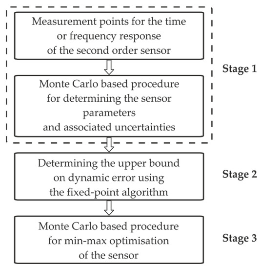
Figure 1.
Block diagram of the procedure for minimising the dynamic error.
Section 3 is devoted to the synthesis of mathematical models of the second-order sensors. Our MC-based procedure for determining the parameters and associated uncertainties forms the original contribution of this study.
The second stage involves the determination of the UBDE using the FPA. This algorithm is based on the step responses of the considered sensor and corresponding reference, which forms a comparison model for the determination of the UBDE. The procedure used to calculate the UBDE with the FPA is discussed in Section 4.
The third stage is our MC-based procedure for min–max optimisation of the sensor. Predetermined ranges are considered for each parameter of the mathematical model of the sensor. The parameter values for the sensor model are determined based on these ranges, finally resulting in the minimal value of the UBDE. The proposed MC-based procedure for minimising the dynamic error is discussed in detail in Section 5.
The transfer function for second-order sensors is represented by the following formula:
where is the frequency [Hz], is the static sensitivity coefficient [V], is the damping factor (dimensionless), and , where is the natural undamped frequency [Hz].
The inverse Laplace transformation, after multiplying by , gives the following step response:
In the time domain, the parameters and are represented by the following formulas [28]:
and
where and denote the overshoot [V] and period of the damped vibrations [s], respectively [34]. Equations (3) and (4) are used to apply the MC method in the time domain.
The amplitude is determined as the modulus based on the complex frequency response , which corresponds to the transfer function represented by Equation (1). The amplitude response is expressed as follows:
In the frequency domain, the parameters and are defined as follows:
and
where denotes the resonant peak [V], and
where denotes the resonant frequency [Hz] [35,36].
Equations (7) and (8) form the basis for applying the MC method in the frequency domain.
2. Procedure for Modelling the Second Order Sensors Using the Monte Carlo Method
The modelling procedure for the second-order sensors in the time domain can be divided into several stages, as described below.
Stage 1: The vector of parameters
is intuitively determined for the time vector
based on the measurement points of the step response
where denotes the number of measurement points [23].
The vector in Equation (9) is determined for the assumed parametric model
Stage 2: Determination of the number of MC draws . The lowest number of draws is determined using the following formula:
based on the guidelines included in [37,38], where is the assumed confidence level and is generally set to 0.95. The successive draws are denoted by .
Stage 3: Determination of the draw ranges for the parameters , and , which should be symmetric around the values of the following parameters: , and (Figure 2). For the determined draw ranges, we expect that there will be parameters of the model given by Equation (1) for which the minimum value of the regression error can be obtained. The values of the parameters that minimise the modelling error are denoted as and
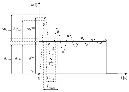
Figure 2.
Example of determining the draw ranges for parameters , and .
Stage 4: Selection of the type of pseudo-random number generator.
Based on Figure 2, it can be assumed that for the model in Equation (1), with parameter values close to , and , there is the greatest probability of obtaining the parameters: , and It, therefore, seems reasonable to choose a generator with a normal distribution [41], as shown in Figure 3.
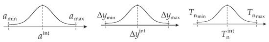
Figure 3.
Application of the generator with a normal distribution for the execution of MC draws.
We denote the function executing the pseudo-random number generator by prng, and estimates of the parameters: and by the symbols: and The following equations show how the function prng is used:
and
Stage 5: Determination of the matrix Φ based on the randomly selected values for the parameters: , and The matrix Φ is obtained by substituting the above parameters into the model of the step response in Equation (12) for the particular values of the vector t. The matrix Φ is given by the formula:
Stage 6: Determination of the matrix Δ associated with the model error. This matrix is determined by subtracting the transposed vector in Equation (11) from the particular columns in the matrix given by Equation (17). We then have:
Stage 7: Determination of the vector representing the sum of the squared errors for each column of the matrix . This vector has the following form:
Stage 8: Determination of the minimum value of the vector and the corresponding drawing number . The parameters: , and resulting from the value are assumed to represent the optimal solution to the regression task executed based on the corresponding measurement points.
Stage 9: The modelling error is calculated for the particular measurement points
Stage 10: Determination of the uncertainty of regression using the MC method:
where
Stage 11: Determination of the uncertainties associated with the parameters: , and using the following formula:
where denotes the corresponding optimal parameters, and the mean [38] is given by the simple formula:
The modelling procedure for second-order sensors in the frequency domain can be divided into the following stages [27]:
Stage 1: Substitution of Equations (6) and (7) into Equation (5), to give the function
Stage 2: Intuitive estimation of the approximate values of the parameters: , and based on the measurement points for the amplitude response (Figure 4).
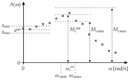
Figure 4.
Example of determining of the draw ranges for parameters and .
Stage 3: Determination of the number of MC draws . The minimum value of is calculated using Equation (11).
Stage 4: Determination of the draw ranges for the parameters: , and , which should be symmetric around the parameters: , and (Figure 4). The parameter values that minimise the error are denoted below by the symbols: , and
Stage 5: Selection of a pseudo-random number generator.
The ranges of the MC draws for the parameters: , and are determined in an analogous way, as shown in Figure 3.
Stage 6: Determination of the matrix:
where is the number of measurement points of the amplitude response . The matrix is determined by substituting the parameters: and into Equation (5) for the particular items where . The parameters: , and are obtained during the successive MC draws: .
Stage 7: Determination of the matrix corresponding to the modelling error, using the formula:
where . The subsequent rows of the matrix Δ reflect the modelling error for the particular pulsations .
Stage 8: Determination of the following vector
where the elements are the sum of the squared errors for each column of the matrix .
Stage 9: Determination of the minimum value of the parameter based on the vector and the corresponding draw number . The parameters: , and which correspond to the value of the parameter , are assumed to be the optimal solutions for the regression of the sensor amplitude response.
Stage 10: Determination of the parameters: and using Equations (7) and (8), respectively.
Stage 11: Determination of the regression uncertainty using the MC method, according to the following formula:
where the mean is
Stage 12: Determination of the uncertainties: , and for the particular parameters: , and using the formula:
where
and corresponds to the particular sensor parameters.
Stage 13: Determination of the complex uncertainties: and associated with the parameters: and based on the following formulae:
and
where the partial derivatives: and are determined using Equation (6), and the derivatives: , and are calculated using Equation (7) [38].
3. Determining the UBDE Using the FPA
Taking into account the test signal constrained in the magnitude and time [5,9,16], and the integral-square criterion (ISC), the UBDE is defined as follows:
where while and denote the constrained test signal. The function is defined, as follows:
where and denote the total step response and time for the steady state of the sensor [9]. The above test signal produces the UBDE which is defined by Equation (34). The total step response is given by the formula:
where is defined in Equation (2), while denotes the step response of the reference used to determine the UBDE. A simple approach is to use a low-pass filter with the bandwidth corresponding to the operating range of the considered sensor [7,18]. The order of the filter should be as high as possible. However, it is limited by the computational possibilities of the mathematical software used for the corresponding calculations.
The value of time is selected to be equal to the steady state of the total step response.
In order to calculate the UBDE according to Equation (34), it is necessary to determine the signal . This signal is obtained using the FPA, as follows:
- Calculate the function according to Equation (35).
- Determine the initial signalwhere denotes the magnitude constraint, and the symbol corresponds to the signum function.
- Determine the input signalfor where denotes the number of iterations selected in advance [9,19].
The final solution, denoted by the symbol: corresponds to the signal , which is included in Equation (34). The signal is the basis for determination of the UBDE. To correct the UBDE by the value resulting from the uncertainties: , and it is necessary to consider the following ranges defined by a uniform distribution: and . For this purpose, the MC method is applied as described in Section 3, except that a pseudo-random number generator with a uniform distribution is used. The corrected UBDE value is denoted below in the following as . The parameters corresponding to this error are denoted by the symbols: , and , while the associated uncertainties are denoted as , and .
4. Monte Carlo Based Procedure for Minimising the Error
When we have obtained the parameters: , and the associated uncertainties: , and for the corresponding it is then possible to implement the min–max optimisation procedure. This procedure is carried out to determine these parameters for the sensor model for their predetermined ranges of variability. The minimum value of the UBDE, defined by Equation (34), can be obtained for these ranges. This value is denoted below in the following as UBDEmin. We assume a uniform distribution for the particular ranges of parameters involved in the optimisation procedure. For these defined ranges, we use the MC method to determine the value of the parameters, which minimise the UBDE according to the ISC.
Figure 5 shows the block diagram for the proposed optimisation procedure.
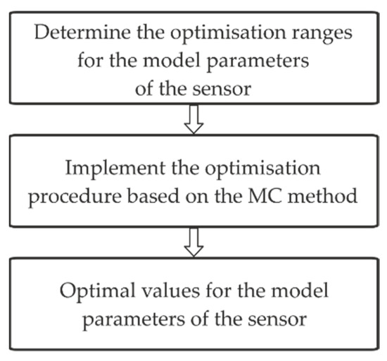
Figure 5.
Block diagram for the optimisation procedure.
The parameter ranges are assumed in advance in the first stage of the proposed procedure. An optimisation is performed in the second stage by applying the MC method, based on a pseudo-random number generator with a uniform distribution. We use the notations , and for the parameters of the second-order sensor that are obtained as a result of applying the optimisation procedure. The uncertainties associated with these parameters are denoted as follows: , and . The lowest possible value of the error, defined by Equation (34), can be obtained using the optimal values of the sensor parameters. The highest value of the accuracy for the considered sensor corresponds to the lowest error determined in this way.
5. Materials and Methods
In this section, we describe the application of the proposed procedure in the frequency domain to the example of the Althen 731-207 accelerometer. Intuitive values for the MC method are set to , and (Figure 4). These values were obtained based on the measurement points of the amplitude response. Then, the minimum and maximum range for the deviation of the above parameters are established as follows: , and .
To determine the parameters: and , a normally distributed pseudo-random number generator (a Box-Muller generator) was used. A number of MC trials equal to was carried out, and the MC and the following results were obtained from the simulation: , and Then, using Equations (6) and (7), the following values were calculated: and Hz. The uncertainty , determined using Equation (27), was equal to 0.02318 , while the uncertainties were obtained using Equation (31) as and The complex uncertainties and were obtained using Equations (32) and (33) as and respectively.
The parameters: , and the associated uncertainties: , were determined for the ranges: and corresponding to a uniform distribution. A tenth-order Butterworth filter was applied as a reference to determine the [19,27]. The time corresponding to the steady state of the total step response was equal to ms. Based on the results of applying our MC method and the FPA, the was obtained as equal to . The corresponding accelerometer parameters and associated uncertainties were as follows: , and .
The last step of the proposed procedure involves the optimisation process described in Section 5. The optimisation ranges for the parameters: and were determined in relation to the maximum tolerance of the parameter , which was set to the range Based on the amplitude response, given by Equation (6), the following ranges: and were obtained for the parameters: and , respectively. The value of the parameter was assumed to be equal to the value of parameter since it is evident that as this parameter increases, the UBDE also increases. The results of the min–max optimisation process were obtained as follows: and Finally, the UBDEmin was found to be equal to , while the associated uncertainties were as follows: and .
Our results indicate that the value of UBDE increases as the parameter is increased. A comparison of the UBDEmin () and () demonstrates the influence of the min–max optimisation on the error UBDE. This influence is seen in a reduction in the UBDE of 2.73% as a result of applying the optimisation procedure to the Althen 731-207 accelerometer. The reduction in UBDE corresponds to the increase in the dynamic accuracy of the accelerometer.
6. Validation of the Proposed Procedure
The proposed procedure and the results presented in Section 5 were validated using a digital signal processor (DSP) of type TMS320C6713 [46]. This processor was programmed in the C language to follow the numerical procedures presented in Section 2, Section 3 and Section 4. The use of DSP made it possible to process the measurement points in real time, and both the time and frequency characteristics were obtained.
Figure 6 shows the relationship between the UBDEmin and the testing time for the Althen 731-207 accelerometer, obtained using MathCad 15 (solid line) and DSP (dotted line).
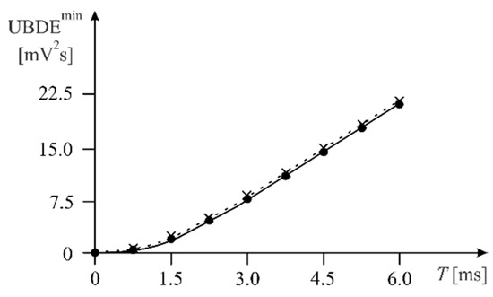
Figure 6.
Relationship between the UBDEmin and the time T for the Althen 731-207 accelerometer testing; MathCad (solid line), DSP (dotted line).
Figure 6 shows that when DSP was used, slightly higher (approx. 2%) UBDEmin values were obtained. The tests were carried out for varying values of the time , which was increased in steps of 0.75 s.
This difference is due to the numerical calculation methods used in MathCad and in DSP (implemented in the C programming language). However, it should be stated that the results obtained with DSP are very approximated with the results obtained with the computer simulation. It should also be noted that the use of DSP allows the proposed min–max optimisation to be implemented in real time, i.e., by combining a practical experiment that allows us to determine time or frequency characteristics with the numerical calculations.
7. Conclusions
The results presented in Section 6 from modelling the Althen 731-207 accelerometer confirm that the proposed procedure can be effectively applied to both scientific and engineering applications. Our procedure involves the use of two numerical methods: FPA and MC. The first is an iterative algorithm with a high degree of convergence and computational efficiency, while the second one is recommended by JCGM guides and can be straightforwardly implemented using mathematical and computational programs (MathCad, MATLAB, C, etc.). The most important finding is that the proposed procedure can be used for modelling in both the time and frequency domains.
The solutions presented in this paper for second-order sensors can be extended to sensors with other dynamic orders; however, this requires the derivation of the relevant mathematical formulae which describe the time and frequency responses of the sensor. In addition to the transfer function used in this study as the basis for deriving the mathematical formulae in the time and frequency domains, it is also possible to use a description of the sensor using a state observer.
The procedure presented in this paper can be implemented using a digital signal processor, although this would require the integral equations presented in Section 3 to be converted to their digital counterparts. In addition, it would be necessary to convert the source code of the algorithm described in Section 2 to codes appropriate to the digital signal processor.
Author Contributions
Conceptualization, K.T.; methodology, K.T., M.K. and K.O.; software, K.T.; validation, K.T., M.K. and K.O.; formal analysis, K.T., M.K. and K.O.; investigation, K.T., M.K. and K.O.; resources, K.T., M.K. and K.O.; data curation, K.T., M.K. and K.O.; writing—original draft preparation, K.T.; writing—review and editing, K.T., M.K. and K.O.; visualization, K.T., M.K. and K.O.; supervision, K.T., M.K. and K.O.; project administration, K.T.; funding acquisition, K.T., M.K. and K.O. All authors have read and agreed to the published version of the manuscript.
Funding
This research was conducted at the Faculty of Electrical and Computer Engineering, Cracow University of Technology, and was financially supported by the Ministry of Science and Higher Education, Republic of Poland (grant no. E-3/2021).
Institutional Review Board Statement
Not applicable.
Informed Consent Statement
Not applicable.
Data Availability Statement
Not applicable.
Conflicts of Interest
The authors declare no conflict of interest.
References
- Gao, X.; Gao, G.; Ren, H.; Chen, D.; He, C. Learning Bayesian network parameters via minimax algorithm. Int. J. Approx. Reason. 2019, 108, 62–75. [Google Scholar] [CrossRef]
- Pradhan, P.; Behera, P.Q.; Ray, B.N.B. Maximin Optimization Problem Subject to Min-Product Fuzzy Relation Inequalities with Application in Supply and Demand Scheme. Int. J. Adv. Sci. Technol. 2020, 29, 1619–1628. [Google Scholar]
- Punia, P.; Kaur, M. Various Genetic Approaches for Solving Single and Multi-Objective Optimization Problems: A Review. Int. J. Adv. Res. Comput. Sci. Softw. Eng. 2013, 3, 1014–1020. [Google Scholar]
- Gorecki, H. Optimization and Control of Dynamic Systems; Springer: Berlin/Heidelberg, Germany, 2018; ISBN 978-3-319-62646-8. [Google Scholar]
- Zhao, T.; Ramos, A.S.; Paulino, G.H. Material nonlinear topology optimization considering the von Mises criterion through an asymptotic approach: Max strain energy and max load factor formulations. Int. J. Num. Meth. Eng. 2019, 118, 804–828. [Google Scholar] [CrossRef]
- Hessling, J.P. A Novel Method of Estimating Dynamic Measurement Errors. Meas. Sci. Technol. 2006, 17, 173–182. [Google Scholar] [CrossRef]
- Layer, E. Mapping Error of Linear Dynamic Systems Caused by Reduced-Order Model. IEEE Trans. Instrum. Meas. 2001, 50, 792–800. [Google Scholar] [CrossRef]
- Wang, C.; Qiu, Z.; He, Y. Fuzzy interval perturbation method for uncertain heat conduction problem with interval and fuzzy parameters. Int. J. Num. Meth. Eng. 2009, 104, 330–346. [Google Scholar] [CrossRef]
- Honig, M.L.; Steiglitz, K. Maximizing the output energy of a linear channel with a time and amplitude limited input. IEEE Trans. Inform. Theory 1992, 38, 1041–1052. [Google Scholar] [CrossRef][Green Version]
- Han, R.; Wang, R.; Zeng, G. Identification of Dynamical Systems Usinga Broad Neural Network and Particle Swarm Optimization. IEEE Access 2020, 8, 132592–132602. [Google Scholar] [CrossRef]
- Pintelon, R.; Schoukens, J. System Identification: A Frequency Domain Approach, 2nd ed.; John Wiley & Sons: Hoboken, NJ, USA, 2012; ISBN 978-0-470-64037-1. [Google Scholar]
- Shua, Y.; Huanga, J.; Donga, Y.; Takeuchi, Y. Mathematical modeling and bifurcation analysis of pro- and anti-tumor macrophages. Appl. Math. Model. 2020, 88, 758–773. [Google Scholar] [CrossRef]
- Shestakov, A.L. Dynamic Measuring Methods: A Review. Acta IMEKO 2019, 8, 64–76. [Google Scholar] [CrossRef]
- Zhu, B.; Pei, H.; Yang, Q. An intelligent response surface method for analyzing slope reliability based on Gaussian process regression. Int. J. Numer. Anal. Methods Geomech. Wiley 2019, 43, 2431–2448. [Google Scholar] [CrossRef]
- Fathi, A. Time functions revisited. Int. J. Geom. Methods Mod. Phys. 2015, 12, 1–13. [Google Scholar] [CrossRef]
- Rutland, N.K. The principle of matching: Practical Conditions for Systems with Inputs Restricted in Magnitude and Rate of Change. IEEE Trans. Autom. Control 1994, 39, 550–553. [Google Scholar] [CrossRef]
- Layer, E. Modelling of Simplified Dynamical Systems; Springer: Berlin/Heidelberg, Germany, 2002; ISBN 978-3-642-56098-9. [Google Scholar]
- Tomczyk, K. Application of genetic algorithm to measurement system calibration intended for dynamic measurement. Metrol. Meas. Syst. 2006, 13, 93–103. [Google Scholar]
- Shukla, D.P.; Tiwari, V. Fixed point algorithms using iteration technique. J. Interdiscip. Math. 2019, 22, 581–591. [Google Scholar] [CrossRef]
- Hirvoas, A.; Prieur, C.; Arnaud ECaleyron, F.; Zuniga, M.M. Quantification and reduction of uncertainties in a wind turbine numerical model based on a global sensitivity analysis and a recursive Bayesian inference approach. Int. J. Num. Meth. Eng. 2021, 122, 2528–2544. [Google Scholar] [CrossRef]
- Gromczak, K.; Gaska, A.; Ostrowska, K.; Sladek, J.; Harmatys, W.; Gaska, P.; Gruza, M.; Kowalski, M. Validation model for coordinate measuring methods based on the concept of statistical consistency control. Precs. Eng. 2016, 45, 414–422. [Google Scholar] [CrossRef]
- Huerto-Cardenas, H.E.; Leonforte, F.; Aste, N.; Del Pero, C.; Evola, G.; Costanzo, G.; Lucchi, E. Validation of dynamic hygrothermal simulation models for historical buildings: State of the art, research challenges and recommendations. Build. Environ. 2020, 180, 107081. [Google Scholar] [CrossRef]
- Jensen, H.; Jerez, D.; Beer, M. A general two-phase Markov chain Monte Carlo approach for constrained design optimization: Application to stochastic structural optimization. Comput. Methods Appl. Mech. Eng. 2021, 373, 113487. [Google Scholar] [CrossRef]
- Guimarães Couto, P.R.; Carreteiro Damasceno, J.; de Oliveira, S.P. Monte Carlo Simulations Applied to Uncertainty in Measurement. In Theory and Applications of Monte Carlo Simulations; Chan, V., Ed.; IntechOpen: London, UK, 2013; pp. 27–51. [Google Scholar]
- Harris, P.M.; Cox, M.G. On a Monte Carlo Method for Measurement Uncertainty Evaluation and its Implementation. Metrologia 2014, 51, 176–182. [Google Scholar] [CrossRef]
- Tomczyk, K. Monte Carlo-based Procedure for Determining the Maximum Energy at the Output of Accelerometers. Energies 2020, 13, 1552. [Google Scholar] [CrossRef]
- Mahdiyar, A.; Armaghani, D.J.; Koopialipoor, M.; Hedayat, A.; Abdullah, A.; Yahya, K. Practical Risk Assessment of Ground Vibrations Resulting from Blasting, Using Gene Expression Programming and Monte Carlo Simulation Techniques. Appl. Sci. 2020, 10, 472. [Google Scholar] [CrossRef]
- Wang, X.; Xu, W.; Luo, H.; Lee, Y.K. Theoretical Modeling, Numerical Simulations and Experimental Study of Micro Thermal Convective Accelerometers. J. Microelectromech. Syst. 2019, 28, 790–798. [Google Scholar] [CrossRef]
- Zhao, D.; Gelman, L.; Chu, F.; Ball, A. Novel Method for Vibration Sensor-Based Instantaneous Defect Frequency Estimation for Rolling Bearings Under Non-Stationary Conditions. Sensors 2020, 20, 5201. [Google Scholar] [CrossRef]
- Tian, B.; Zhao, Y.L.; Niu, Z.; Jiang, Z.D.; Zhang, T.Y. The Structure Design and Analysis of Vibration Sensor. Appl. Mech. Mater. 2014, 701, 569–572. [Google Scholar] [CrossRef]
- Xu, F.; Li, X.; Shi, Y.; Li, L.; Wang, W.; He, L.; Liu, R. Recent Developments for Flexible Pressure Sensors: A Review. Micromachines 2018, 9, 580. [Google Scholar] [CrossRef]
- Patra, J.C.; Kot, A.C.; Panda, G. An Intelligent Pressure Sensor Using Neural Networks. IEEE Trans. Instrum. Meas. 2000, 4, 829–834. [Google Scholar] [CrossRef]
- Morris, A.S.; Langari, R. Measurement and Instrumentation, Theory and Application; Elsevier Academic Press: Amsterdam, The Netherlands, 2021; ISBN 9780128171417. [Google Scholar]
- Close, C.M.; Frederick, D.K.; Newell, J.C. Modeling and Analysis of Dynamic Systems; Wiley: Hoboken, NJ, USA, 2001; ISBN 978-0-471-39442-6. [Google Scholar]
- Shan, X.; Song, H.; Zhang, C.; Wang, G.; Fan, J. Linear System Identification and Vibration Control of End-Eector for Industrial Robots. Appl. Sci. 2020, 10, 8537. [Google Scholar] [CrossRef]
- Andreassen, E.; Ferrari, F.; Sigmund, O.; Diaz, A.R. Frequency response as a surrogate eigenvalue problem in topology optimization. Int. J. Num. Meth. Eng. 2017, 113, 1214–1229. [Google Scholar] [CrossRef]
- BIPM, IEC, IFCC, ILAC, ISO, IUPAP, OIML, Guide to the Expression of Uncertainty in Measurement. Supplement 1—Propagation of Distributions Using a Monte Carlo Method. 2008. Available online: https://www.iso.org/standard/50462.html (accessed on 1 November 2008).
- BIPM, IEC, IFCC, ILAC, ISO, IUPAP, OIML, Guide to the Expression of Uncertainty in Measurement. Supplement 2—Extension to any Number of Output Quantities. 2011. Available online: https://www.iso.org/standard/50463.html (accessed on 1 November 2011).
- Sanchez-Sutil, F.; Cano-Ortega, A.; Hernandez, J.C.; Rus-Casas, C. Development and Calibration of an Open Source, Low-Cost Power Smart Meter Prototype for PV Household-Prosumers. Electronics 2019, 8, 878. [Google Scholar] [CrossRef]
- Tomczyk, K. Influence of Monte Carlo Generations Applied for Modelling of Measuring Instruments on Maximum Distance Error. Trans. Inst. Meas. Control 2019, 41, 74–84. [Google Scholar] [CrossRef]
- Wichmann, B.A.; Hill, I.D. Generating Good Pseudo-Random Numbers. Comput. Stat. Data Anal. 2006, 51, 1614–1622. [Google Scholar] [CrossRef]
- Thomas, D.B.; Luk, W.; Leong, P.H.W.; Villasenor, J.D. Gaussian Random Number Generators. ACM Comput. Surv. 2007, 39, 11. [Google Scholar] [CrossRef]
- Dudzik, M.; Tomczyk, K.; Jagiełło, A. Analysis of the Error Generated by the Voltage Output Accelerometer Using the Optimal Structure of an Artificial Neural Network. In Proceedings of the 19th International Conference on Research and Education in Mechatronics (REM’2018), Delft, The Netherlands, 7–8 June 2018. [Google Scholar]
- Segers, J. Analysis Techniques for Racecar Data Acquisition; SAE International: Warrendale, PA, USA, 2014; p. 0768064597. [Google Scholar]
- Ponce-Cruz, P.; Ramírez-Figueroa, F.D. Intelligent Control Systems with LabVIEW; Springer: Berlin/Heidelberg, Germany, 2010; ISBN 978-1-84882-684-7. [Google Scholar]
- Texas Instruments TMS320C6713 Data Sheet. Available online: https://pdf1.alldatasheet.com/datasheet-pdf/view/227375/TI/TMS320C6713.html (accessed on 15 February 2022).


Publisher’s Note: MDPI stays neutral with regard to jurisdictional claims in published maps and institutional affiliations. |
© 2022 by the authors. Licensee MDPI, Basel, Switzerland. This article is an open access article distributed under the terms and conditions of the Creative Commons Attribution (CC BY) license (https://creativecommons.org/licenses/by/4.0/).