
Acoustic Noise-Based Detection of Ferroresonance Events in Isolated Neutral Power Systems with Inductive Voltage Transformers

 , , ,
, , ,  , ,
, ,  ,
,  and
and
Abstract
:1. Introduction
2. Indirect Ferroresonances Detection in MV Isolated-Neutral Power Systems
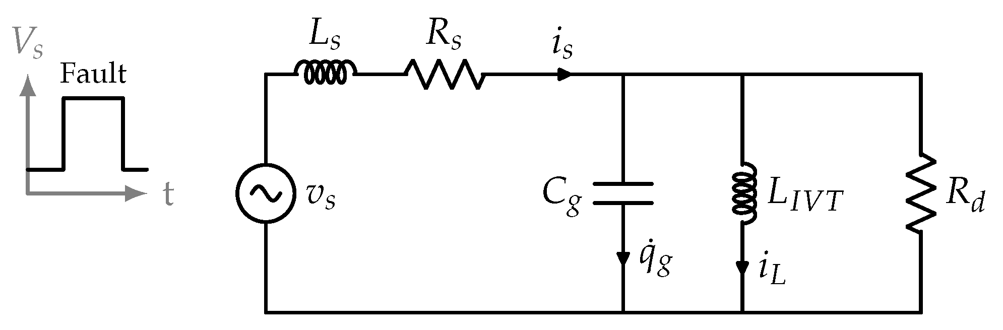
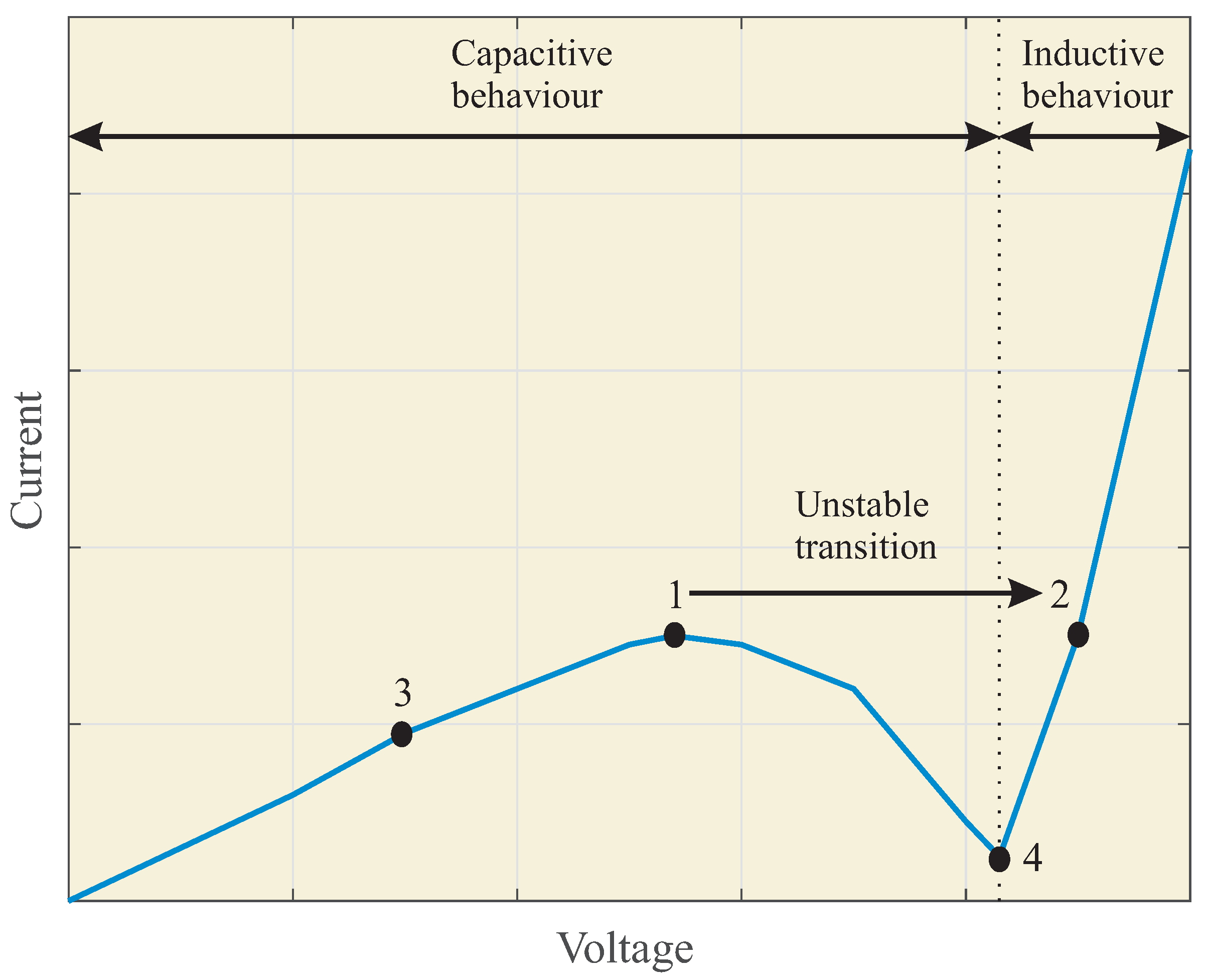
2.1. Phenomenon Description
- High distortions of waveforms, overvoltages, and overcurrents.
- Neutral voltage displacement.
- Overheating of transformers.
- Noise and vibration in transformers.
- Damage to transformer primary winding and electrical equipment.
2.2. Indirect Detection through IVT Vibrations
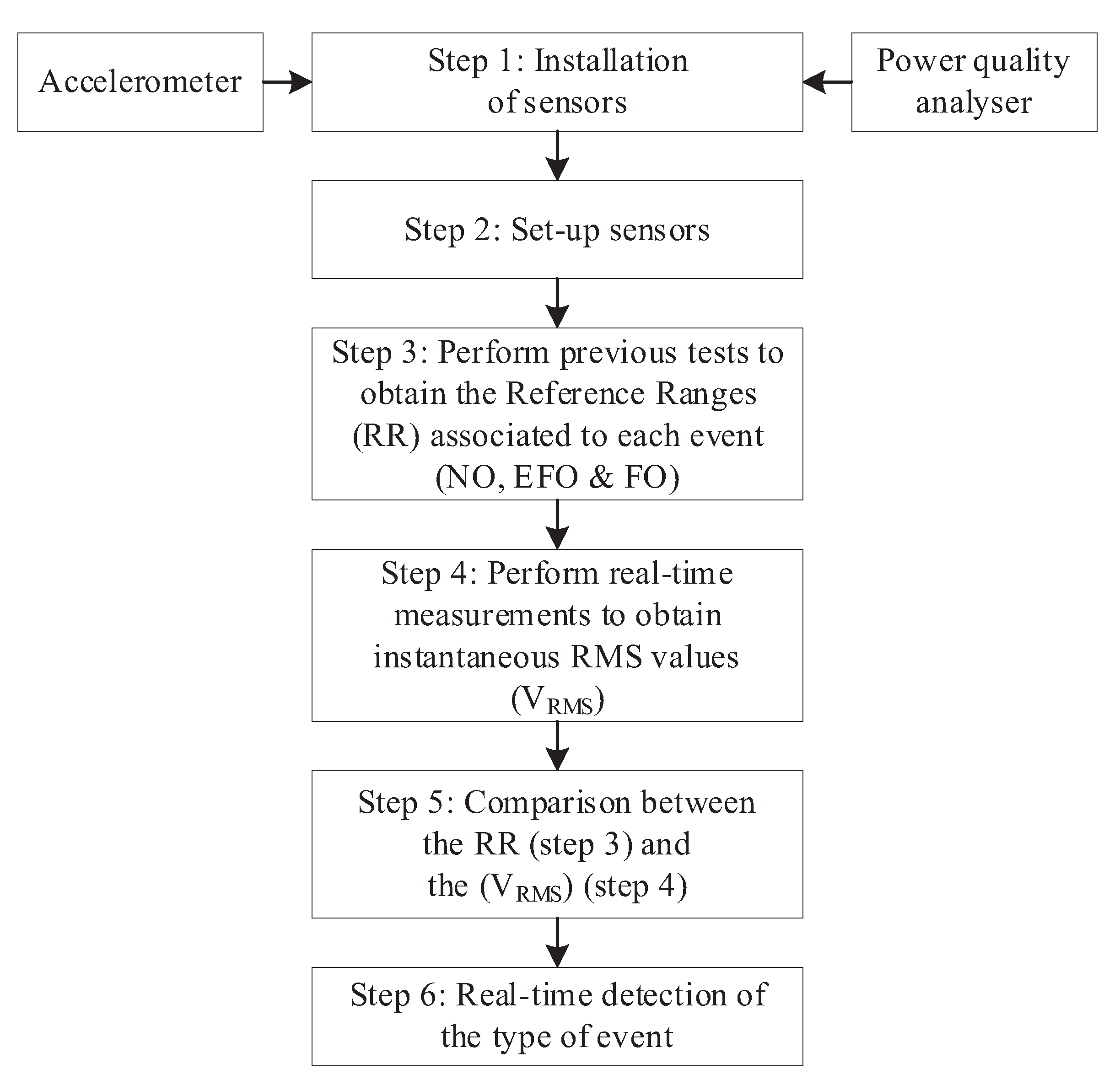
- Step 1: Installing the accelerometers. Three IVTs are used for voltage measurement in isolated neutral power systems. One accelerometer must be located on the IVT case. Safety procedures and isolation levels for medium voltage grids must be accomplished. Special care must be taken to ensure an appropriate mechanical coupling.
- Step 2: Set-up sensors. Sensors must be calibrated to achieve their right operation at the IVT specific place. It will be necessary to calibrate the sensors to adjust the sensitivity, the range of measurements, etc. The auxiliary power supply must also be adjusted.
- Step 3: Perform previous tests to obtain the reference ranges (RR) associated with an IVT electrical event: normal operation (NO), single phase-to-earth fault operation (EFO), and ferroresonance operation (FO).
- -
- Step 3.1: Perform previous tests to measure the vibrations for each electrical event of the IVT.
- -
- Step 3.2: Perform the vibration signal conditioning for each electrical event of the IVT.
- -
- Step 3.3: Perform the discretization of the conditioned vibration signals for each electrical event of the IVT.
- -
- Step 3.4: Perform the equalization of the discretized vibration signals for each electrical event of the IVT.
- -
- Step 3.5: Obtain the RMS vibration signals from the equalized signals associated with each electrical event of the IVT.
- -
- Step 3.6: Obtain the RR associated with each electrical event of the IVT.
- Step 4: Perform real-time measurements to obtain instantaneous RMS values .
- Step 5: Comparison between the RR (Step 3) and the instantaneous RMS values (Step 4).
- Step 6: Real-time detection of the type of event.
3. Indirect Ferroresonance Detection through Acoustic Noise
3.1. Acoustic Noise Sensors for IVT
3.2. Modifications to the Methodology in [32] for Using Microphones as Sensors
- Step 1: The microphone must be placed inside the switchgear, ensuring a proper fixation to the cabinet door.
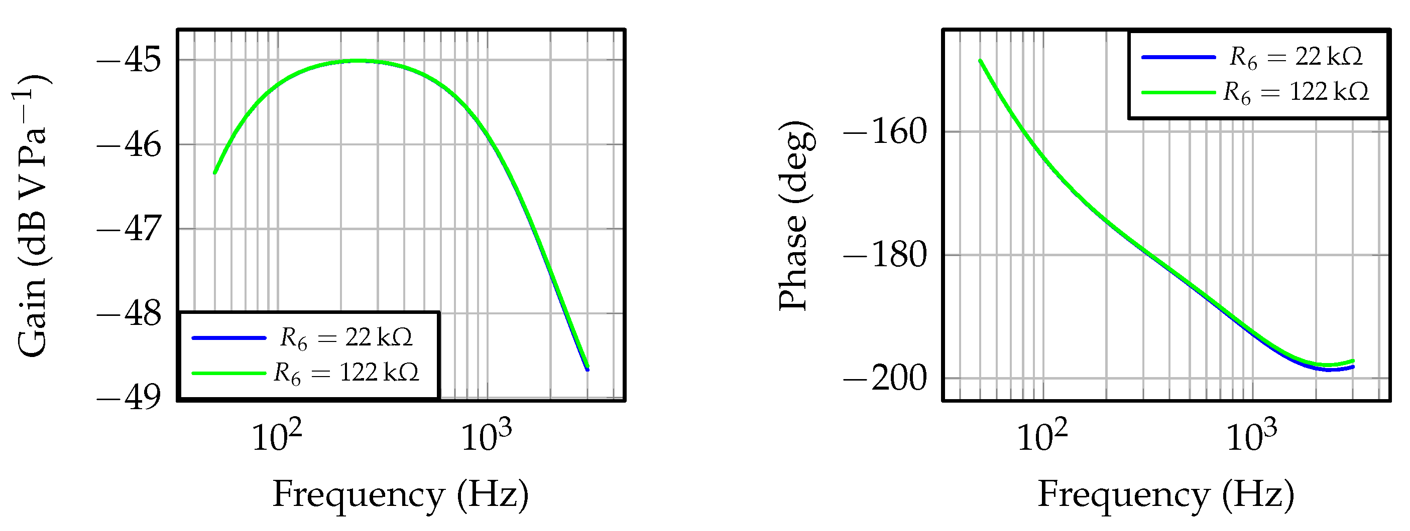
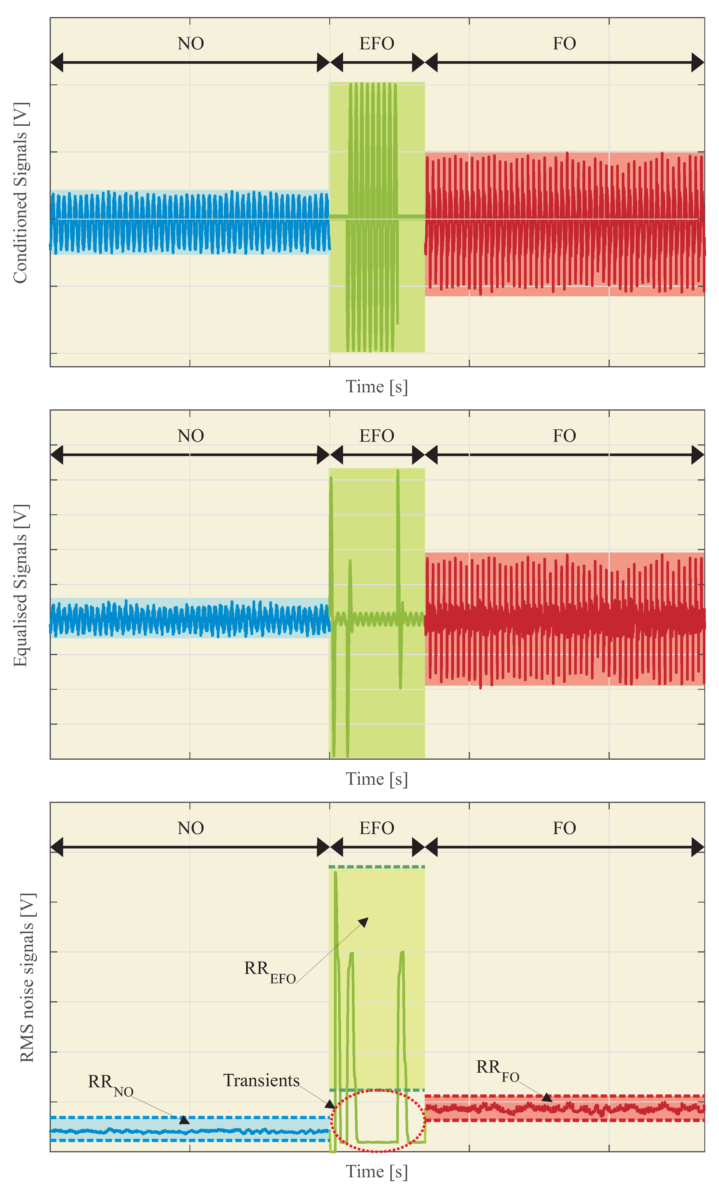
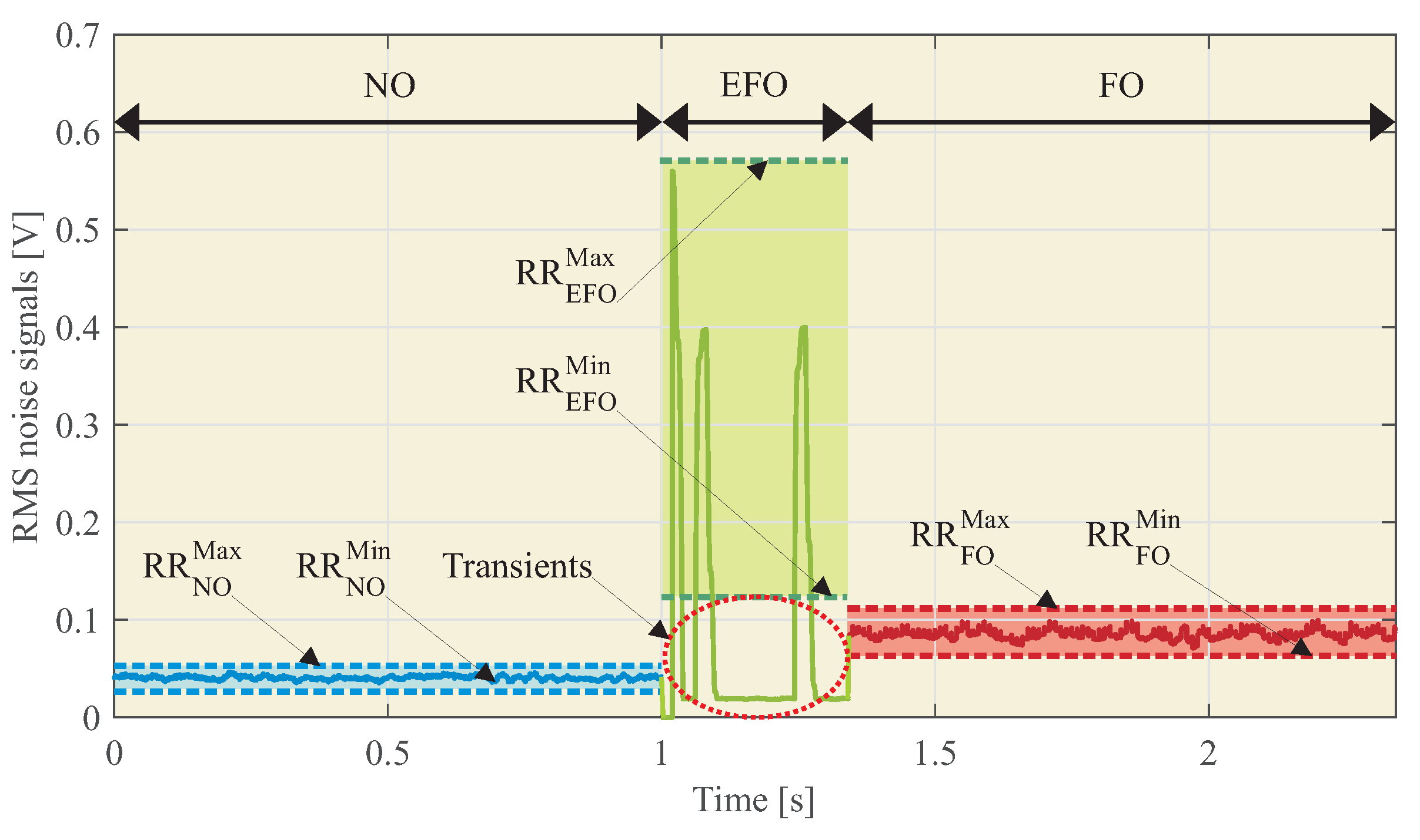
- Step 3.6: The reference ranges, , for detection purposes, must be adjusted to the new sensor. Previous analysis allows the ranges to be approximated, but experimental tests are recommendable for fine tuning. Figure 10 shows an example. The associated with each electrical event i, i.e., , is calculated as the minimum and maximum of the RMS noise signal values. Thus,where i is the electrical event associated with the RMS sound signal: NO, EFO, or FO.The transients during the EFO should be avoided. Therefore,
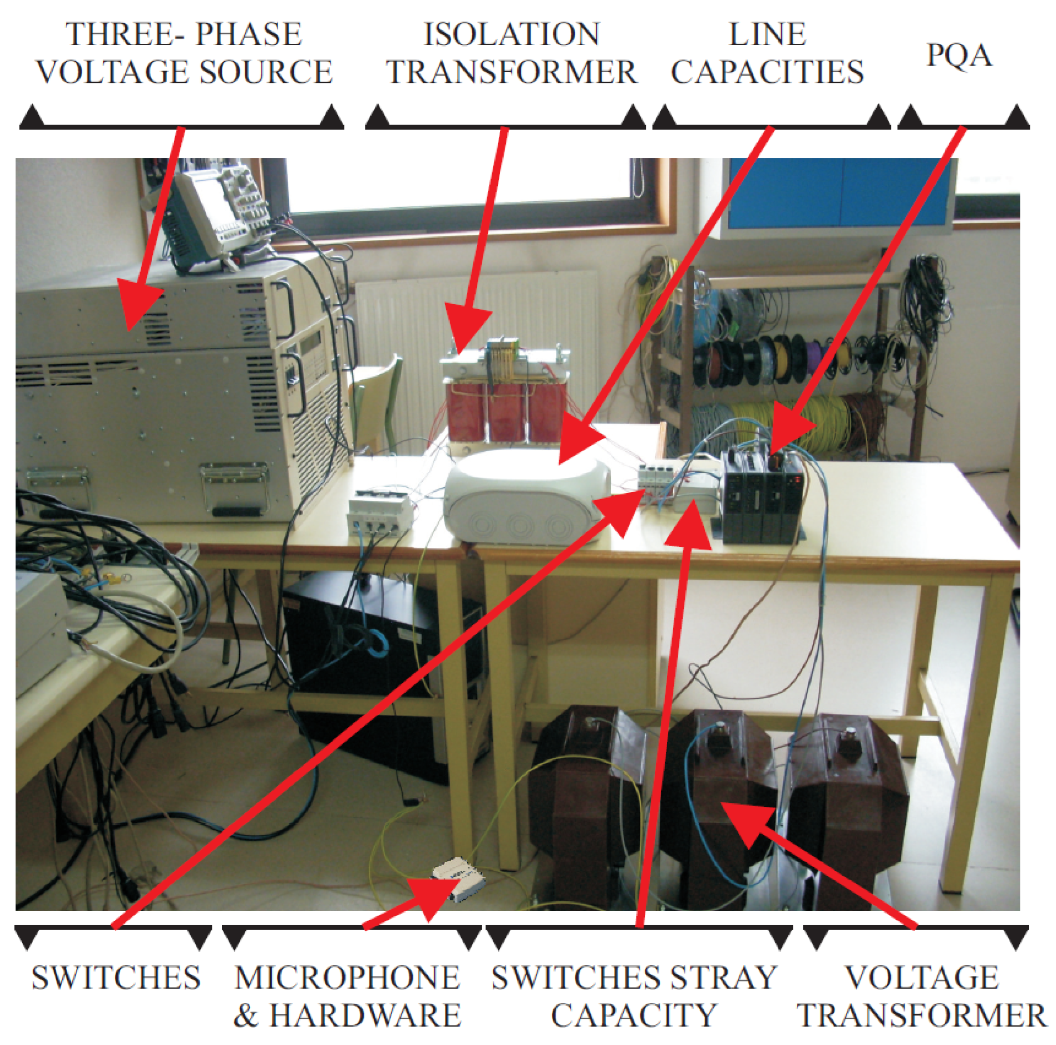
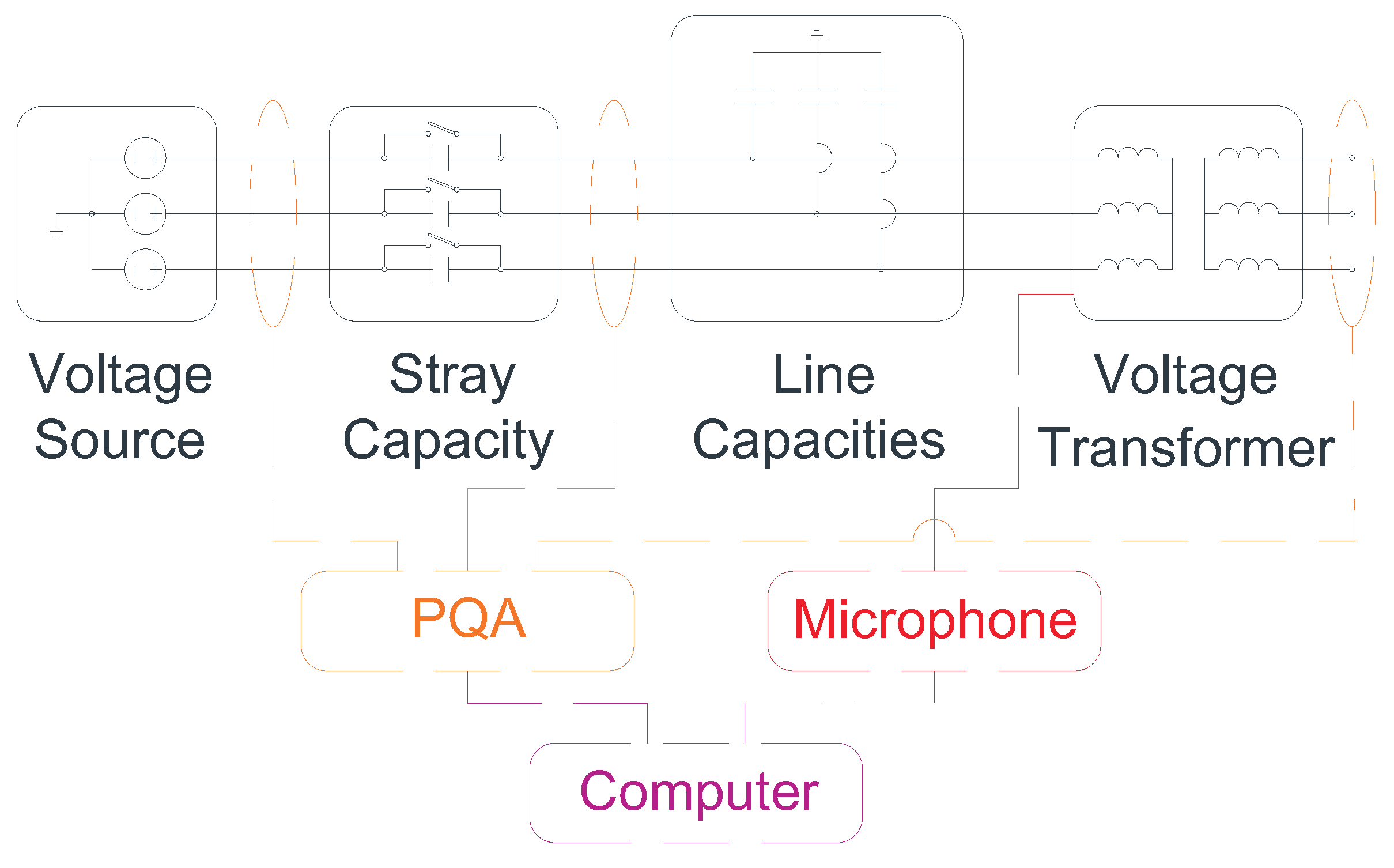
4. Set-Up Facility
5. Experimental Results
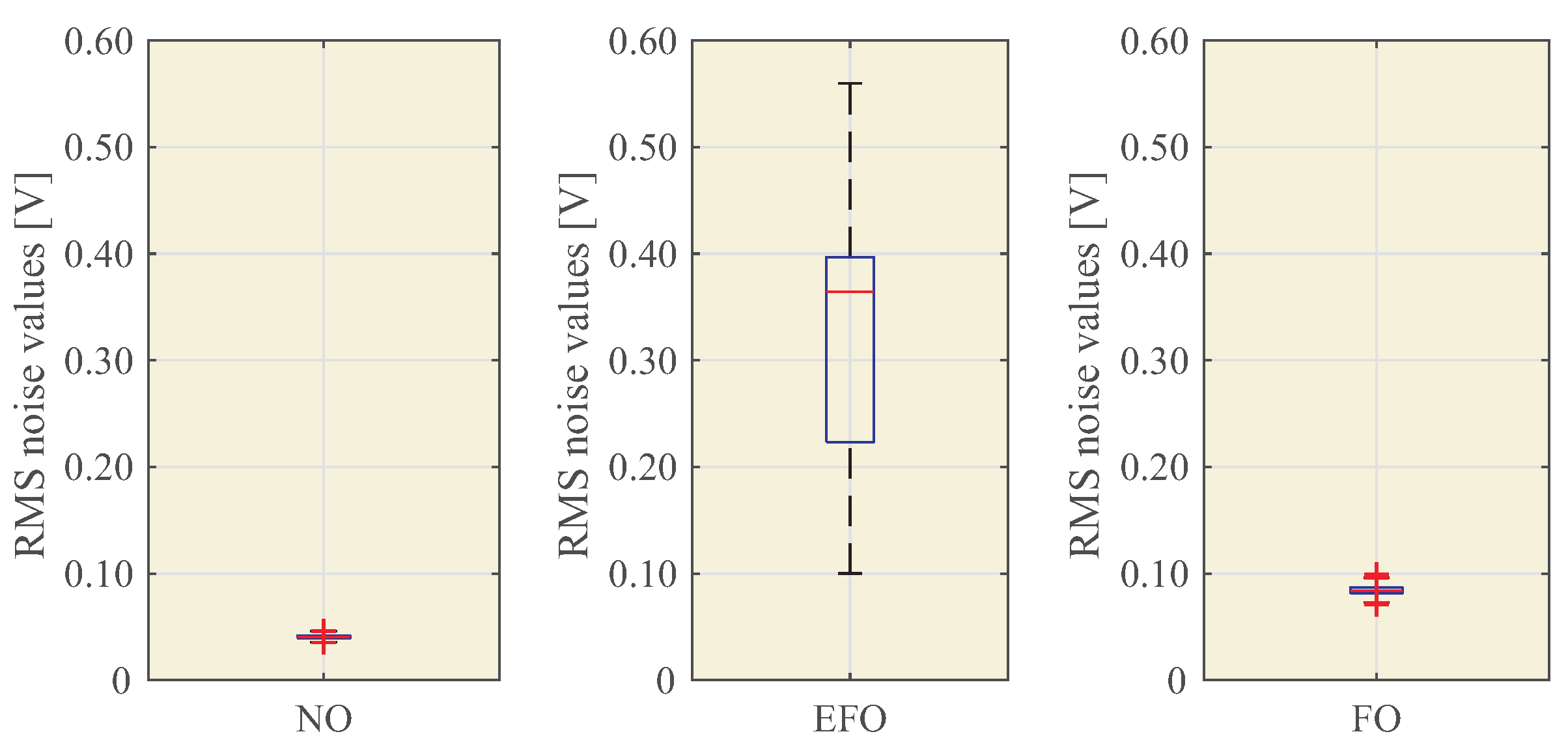
5.1. Indirect Detection Method with Acoustic Noise Sensors
- From 0 to 1 s, the noise signal is in the NO event type.
- From 1 to 1.3 s, the noise signal is in the EFO event type.
- From 1.3 to 2.5 s, the noise signal is in the FO event type.
5.2. Comparison of Indirect Methods with Accelerometers or Microphone
6. Discussion
Author Contributions
Funding
Institutional Review Board Statement
Informed Consent Statement
Acknowledgments
Conflicts of Interest
Abbreviations
| Operational amplifier open-loop gain [dB]. | |
| ADC | Analog-to-digital converter. |
| Bandwidth of the A-weighted noise distribution []. | |
| EFO | Earth fault operation. |
| IVT magnetic flux []. | |
| FET | Field-effect transistor. |
| FO | Ferroresonance operation. |
| Operational gain bandwidth []. | |
| Low-pass filtering transfer function. | |
| Capacitive current []. | |
| Microphone current consumption []. | |
| IVT current []. | |
| Phasorial representation of IVT current []. | |
| Microphone uncompensated current noise spectral density []. | |
| Microphone compensated current noise spectral density []. | |
| Line current []. | |
| Phasorial representation of line current []. | |
| IVT | Inductive voltage transformer. |
| Boltzmann’s constant []. | |
| LPF | Low-pass filter. |
| NO | Normal operation |
| OA | Operational amplifier. |
| PQA | Power quality analyser. |
| PS | Power system. |
| Damping resistor []. | |
| Microphone typical output impedance []. | |
| RMS | Root mean square. |
| RR | Reference range. |
| Reference range for the operation i. | |
| Minimum value of the reference range for the operation i. | |
| Maximum value of the reference range for the operation i. | |
| Typical microphone sensitivity [dB]. | |
| SAR | Successive-approximation register. |
| SNR | Signal-to-noise ratio [dB]. |
| Sound wave pressure []. | |
| Operational amplifier slew rate []. | |
| T | Temperature []. |
| Operational amplifier input noise voltage density []. | |
| Line-to-ground voltage []. | |
| RMS value of line-to-ground voltage []. | |
| Phasorial representation of line-to-ground voltage []. | |
| Line-to-ground reactance []. | |
| IVT reactance []. | |
| Line impedance []. | |
| Microphone output admittance []. |
References
- Chakravarthy, S.; Nayar, C. Series ferroresonance in power systems. Int. J. Electr. Power Energy Syst. 1995, 17, 267–274. [Google Scholar] [CrossRef]
- Ferracci, P. Ferroresonance. Techreport 190. 1998. Available online: https://www.se.com/ww/en/download/document/ECT190/ (accessed on 28 November 2022).
- Price, E. A tutorial on ferroresonance. In Proceedings of the 2014 67th Annual Conference for Protective Relay Engineers, College Station, TX, USA, 31 March–3 April 2014. [Google Scholar] [CrossRef]
- Kruger, S.; de Kock, J. Ferroresonance: A Review of the Phenomenon and Its Effects. In Proceedings of the 2021 Southern African Universities Power Engineering Conference/Robotics and Mechatronics/Pattern Recognition Association of South Africa (SAUPEC/RobMech/PRASA), Potchefstroom, South Africa, 27–29 January 2021. [Google Scholar] [CrossRef]
- De Keulenaer, H. Transient and Temporary Overvoltages and Currents—Annex D: Ferroresonance Effects-Power Quality and Utilisation Guide; Techreport. 2008. Available online: https://studylib.net/doc/18680210/transient-and-temporary-overvoltages-and (accessed on 28 November 2022).
- Mokryani, G.; Haghifam, M.R.; Latafat, H.; Aliparast, P.; Abdollahy, A. Analysis of ferroresonance in a 20kV distribution network. In Proceedings of the 2009 2nd International Conference on Power Electronics and Intelligent Transportation System (PEITS), Shenzhen, China, 19–20 December 2009. [Google Scholar] [CrossRef]
- Janssens, N.; Craenenbroeck, T.V.; Dommelen, D.V.; Meulebroeke, F.V.D. Direct calculation of the stability domains of three-phase ferroresonance in isolated neutral networks with grounded neutral voltage transformers. IEEE Trans. Power Deliv. 1996, 11, 1546–1553. [Google Scholar] [CrossRef]
- Akinrinde, A.; Swanson, A.; Tiako, R. Dynamic Behavior of Wind Turbine Generator Configurations during Ferroresonant Conditions. Energies 2019, 12, 639. [Google Scholar] [CrossRef] [Green Version]
- Mosaad, M.; Sabiha, N.; Abu-Siada, A.; Taha, I. Application of Superconductors to Suppress Ferroresonance Overvoltage in DFIG-WECS. IEEE Trans. Energy Convers. 2022, 37, 766–777. [Google Scholar] [CrossRef]
- Rezaei, S.; Aref, S.; Anaraki, A.S. A review on oscillations in Wind Park due to ferroresonance and subsynchronous resonance. IET Renew. Power Gener. 2021, 15, 3777–3792. [Google Scholar] [CrossRef]
- Solak, K.; Rebiant, W. Modeling of Ferroresonance Phenomena in MV Networks. In Proceedings of the 2018 IEEE Electrical Power and Energy Conference (EPEC), Toronto, ON, Canada, 10–11 October 2018. [Google Scholar] [CrossRef]
- Piasecki, W.; Florkowski, M.; Fulczyk, M.; Mahonen, P.; Nowak, W. Mitigating Ferroresonance in Voltage Transformers in Ungrounded MV Networks. IEEE Trans. Power Deliv. 2007, 22, 2362–2369. [Google Scholar] [CrossRef]
- Heidary, A.; Rouzbehi, K.; Radmanesh, H.; Pou, J. Voltage Transformer Ferroresonance: An Inhibitor Device. IEEE Trans. Power Deliv. 2020, 35, 2731–2733. [Google Scholar] [CrossRef]
- Heidary, A.; Radmanesh, H. Smart solid-state ferroresonance limiter for voltage transformers application: Principle and test results. IET Power Electron. 2018, 11, 2545–2552. [Google Scholar] [CrossRef]
- Mitrea, S.; Adascalitei, A. On the prediction of ferroresonance in distribution networks. Electr. Power Syst. Res. 1992, 23, 155–160. [Google Scholar] [CrossRef]
- Martínez, R.; Manana, M.; Rodríguez, J.I.; Álvarez, M.; Mínguez, R.; Arroyo, A.; Bayona, E.; Azcondo, F.; Pigazo, A.; Cuartas, F. Ferroresonance phenomena in medium-voltage isolated neutral grids: A case study. IET Renew. Power Gener. 2018, 13, 209–214. [Google Scholar] [CrossRef]
- Karaagac, U.; Mahseredjian, J.; Cai, L. Ferroresonance conditions in wind parks. Electr. Power Syst. Res. 2016, 138, 41–49. [Google Scholar] [CrossRef]
- Mosaad, M.I.; Sabiha, N.A. Ferroresonance Overvoltage Mitigation Using STATCOM for Grid-connected Wind Energy Conversion Systems. J. Mod. Power Syst. Clean Energy 2022, 10, 407–415. [Google Scholar] [CrossRef]
- Rezaei, S. An adaptive bidirectional protective relay algorithm for ferroresonance in renewable energy networks. Electr. Power Syst. Res. 2022, 212, 108625. [Google Scholar] [CrossRef]
- Azcondo, F.J.; Bayona, E.; Branas, C.; Casanueva, R.; Diaz, F.; Pigazo, A.; Mañana, M.; Minguez, R.; Alvarez, M. Electronic System and Method for the Mitigation of Ferroresonances in Voltage Transformers. ES 2756923B2, 9 February 2021. [Google Scholar]
- Solak, K.; Rebizant, W.; Kereit, M. Detection of Ferroresonance Oscillations in Medium Voltage Networks. Energies 2020, 13, 4129. [Google Scholar] [CrossRef]
- Negara, I.M.Y.; Hernanda, I.G.N.S.; Asfani, D.A.; Fahmi, D.; Hakim, L.L.; Putra, I.G.A.P. Identification of Ferroresonance on Transformer using Wavelet Transformatio. In Proceedings of the 2019 2nd International Conference on High Voltage Engineering and Power Systems (ICHVEPS), Denpasar, Bali, 1–4 October 2019. [Google Scholar] [CrossRef]
- Mokryani, G.; Haghifam, M.R. Application of wavelet transform and MLP neural network for Ferroresonance identification. In Proceedings of the 2008 IEEE Power and Energy Society General Meeting-Conversion and Delivery of Electrical Energy in the 21st Century, Pittsburgh, PA, USA, 20–24 July 2008. [Google Scholar] [CrossRef]
- Sharbain, H.A.; Osman, A.; El-Hag, A. Detection and identification of ferroresonance. In Proceedings of the 2017 7th International Conference on Modeling, Simulation, and Applied Optimization (ICMSAO), Sharjah, United Arab Emirates, 4–6 April 2017. [Google Scholar] [CrossRef]
- Wahyudi, M.; Negara, I.M.Y.; Asfani, D.A.; Hernanda, I.G.N.S.; Fahmi, D. Application of wavelet cumulative energy and artificial neural network for classification of ferroresonance signal during symmetrical and unsymmetrical switching of three-phases distribution transformer. In Proceedings of the 2017 International Conference on High Voltage Engineering and Power Systems (ICHVEPS), Denpasar, Bali, 2–5 October 2017. [Google Scholar] [CrossRef]
- Correa, J.; Vega, J. Protection Relay for Secondary Ferroresonance Suppression in Coupling Capacitor Voltage Transformers. In Proceedings of the 2020 IEEE PES Transmission & Distribution Conference and Exhibition-Latin America T&D LA), Chicago, IL, USA, 12–15 October 2020. [Google Scholar] [CrossRef]
- Kong, H.; Zhang, B.; Bo, Z. A novel ferroresonance recognition method based on the excitation characteristic of potential transformer. In Proceedings of the 2014 International Conference on Power System Technology, Chengdu, China, 20–22 October 2014. [Google Scholar] [CrossRef]
- Dong, X.; Li, X.; Bo, Z.; Chatfield, R.; Klimek, A. Method and System for Online Ferroresonance Detection. U.S. Patent 9246326B2, 31 January 2016. [Google Scholar]
- Piasecki, W. Protection System for Voltage Transformers. U.S. Patent 20110062797 A1, 17 March 2011. [Google Scholar]
- Misak, S.; Fulnecek, J. The influence of ferroresonance on a temperature of voltage transformers in undeground mines. In Proceedings of the 2017 18th International Scientific Conference on Electric Power Engineering (EPE), Kouty nad Desnou, Czech Republic, 17–19 May 2017. [Google Scholar] [CrossRef]
- Mikhak-Beyranvand, M.; Faiz, J.; Rezaei-Zare, A.; Rezaeealam, B. Electromagnetic and thermal behavior of a single-phase transformer during Ferroresonance considering hysteresis model of core. Int. J. Electr. Power Energy Syst. 2020, 121, 106078. [Google Scholar] [CrossRef]
- Arroyo, A.; Martinez, R.; Manana, M.; Pigazo, A.; Minguez, R. Detection of ferroresonance occurrence in inductive voltage transformers through vibration analysis. Int. J. Electr. Power Energy Syst. 2019, 106, 294–300. [Google Scholar] [CrossRef]
- Dugan, R. Examples of ferroresonance in distribution. In Proceedings of the 2003 IEEE Power Engineering Society General Meeting (IEEE Cat. No.03CH37491), Toronto, ON, Canada, 13–17 July 2003. [Google Scholar] [CrossRef]
- Bukreev, A.; Vinogradov, A.; Bolshev, V.; Panchenko, V. Conductor Identification Using Acoustic Signal Method. Sustainability 2022, 14, 7297. [Google Scholar] [CrossRef]
- IEC 60076-10-1:2016; Power Transformer. Part 10-1: Determination of Sounds Levels. International Electrotechnical Commission: Geneva, Switzerland, 2016.
- 1/2-Inch Infrasound Microphone. Technical Report, Brüel & Kjaer. 2022. Available online: https://www.bksv.com/es/transducers/acoustic/microphones/microphone-cartridges/4964 (accessed on 28 November 2022).
- Watanabe, K.; Kurihara, Y.; Nakamura, T.; Tanaka, H. Design of a Low-Frequency Microphone for Mobile Phones and Its Application to Ubiquitous Medical and Healthcare Monitoring. IEEE Sens. J. 2010, 10, 934–941. [Google Scholar] [CrossRef]
- Corsini, A.; Tortora, C.; Feudo, S.; Sheard, A.G.; Ullucci, G. Implementation of an acoustic stall detection system using near-field DIY pressure sensors. Proc. Inst. Mech. Eng. Part J. Power Energy 2016, 230, 487–501. [Google Scholar] [CrossRef] [Green Version]
- Segovia-Fernandez, J.; Sonmezoglu, S.; Block, S.T.; Kusano, Y.; Tsai, J.M.; Amirtharajah, R.; Horsley, D.A. Monolithic piezoelectric Aluminum Nitride MEMS-CMOS microphone. In Proceedings of the 2017 19th International Conference on Solid-State Sensors, Actuators and Microsystems (TRANSDUCERS), Kaohsiung, Taiwan, 18–22 June 2017. [Google Scholar] [CrossRef]
- Low-Cost, Micropower, SC70/SOT23-8, Microphone Preamplifiers with Complete Shutdown. Technical Report 9-1950. 2012. Available online: https://datasheets.maximintegrated.com/en/ds/MAX4465-MAX4469.pdf (accessed on 28 November 2022).
- Electret Microphone Amplifier-MAX4466 with Adjustable Gain. Technical Report, Adafruit. 2022. Available online: https://www.adafruit.com/product/1063 (accessed on 28 November 2022).
- Datasheet CMA-4544PF-W Electret Condenser Microphone. Technical Report, CUI Devices. 2022. Available online: https://www.cuidevices.com/product/resource/cma-4544pf-w.pdf (accessed on 28 November 2022).
- Caldwell, J. Single-Supply, Electret Microphone Pre-Amplifier Reference Design; Technical Report TIDU765; Texas Instruments Inc.: Dallas, TX, USA, 2015; Available online: https://www.ti.com/lit/ug/tidu765/tidu765.pdf (accessed on 28 November 2022).
- Noise Analysis in Operational Amplifier Circuits. Technical Report SLVA043B. 2007. Available online: https://www.ti.com/lit/an/slva043b/slva043b.pdf (accessed on 28 November 2022).
- Noise in Operational Amplifiers (Video series). Technical Report, TI Precision Labs-Training Videos. 2022. Available online: https://training.ti.com/node/1138803?context=1139747-1139745-14685-1138803 (accessed on 28 November 2022).
- Magnusson, P. Voltage and Current Noise Sources in LTspice.noise Simulations. 2017. Available online: https://axotron.se/blog/voltage-and-current-noise-sources-in-ltspice-noise-simulations/ (accessed on 28 November 2022).
- Successive-Approximation-Register (SAR) Analog-to-Digital Converter (ADC) Input Driver Design; Technical Report; Texas Instruments Inc.: Dallas, TX, USA, 2017; Available online: https://training.ti.com/node/1139106 (accessed on 28 November 2022).
- Ertl, M.; Voss, S. The role of load harmonics in audible noise of electrical transformers. J. Sound Vib. 2014, 333, 2253–2270. [Google Scholar] [CrossRef]
- He, Q.; Fan, C.; Yang, G.; Li, H.; Li, J.; Chen, X. Experimental Analysis of Transformer Core Vibration and Noise under Inter-Harmonic Excitation. Appl. Sci. 2022, 12, 1758. [Google Scholar] [CrossRef]


| Datasheet Param. | Value | Model Param. | Value |
|---|---|---|---|
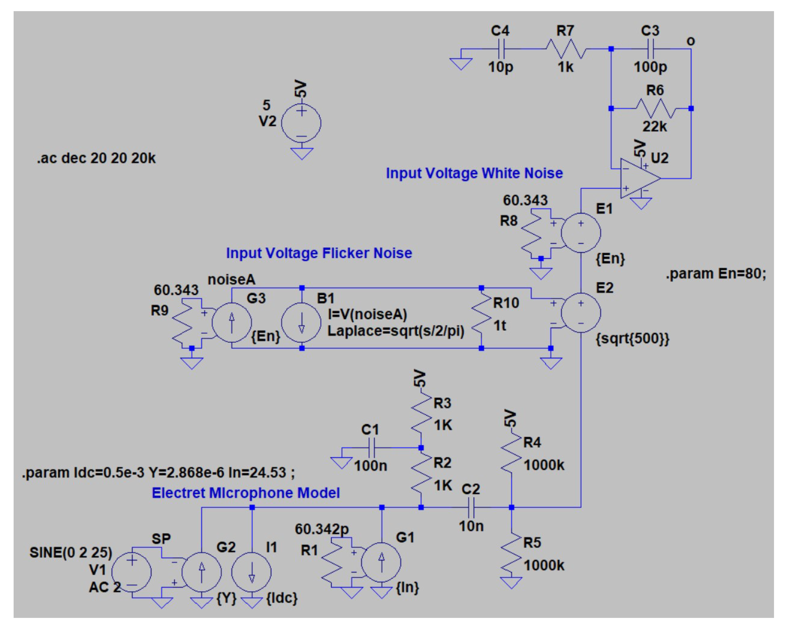
| Sensitivity () | dB | Output admittance () | 2.868 μA/ |
| Output impedance () | 2.2 kΩ | ||
| Signal-to-Noise Ratio () | 60 dB | Current noise | / |
| Current consumption () | spectral density () |
| Datasheet Param. | Value |
|---|---|
| Open-Loop Gain () | 125 dB ( 100 ) |
| Gain Bandwidth () | 125 |
| Slew Rate () | 300 mV μs−1 |
| Input Noise Voltage Density () ( 1 ) | 80 / |
| Voltage noise corner frequency | 500 |
| Element | Description and Technical Data |
|---|---|
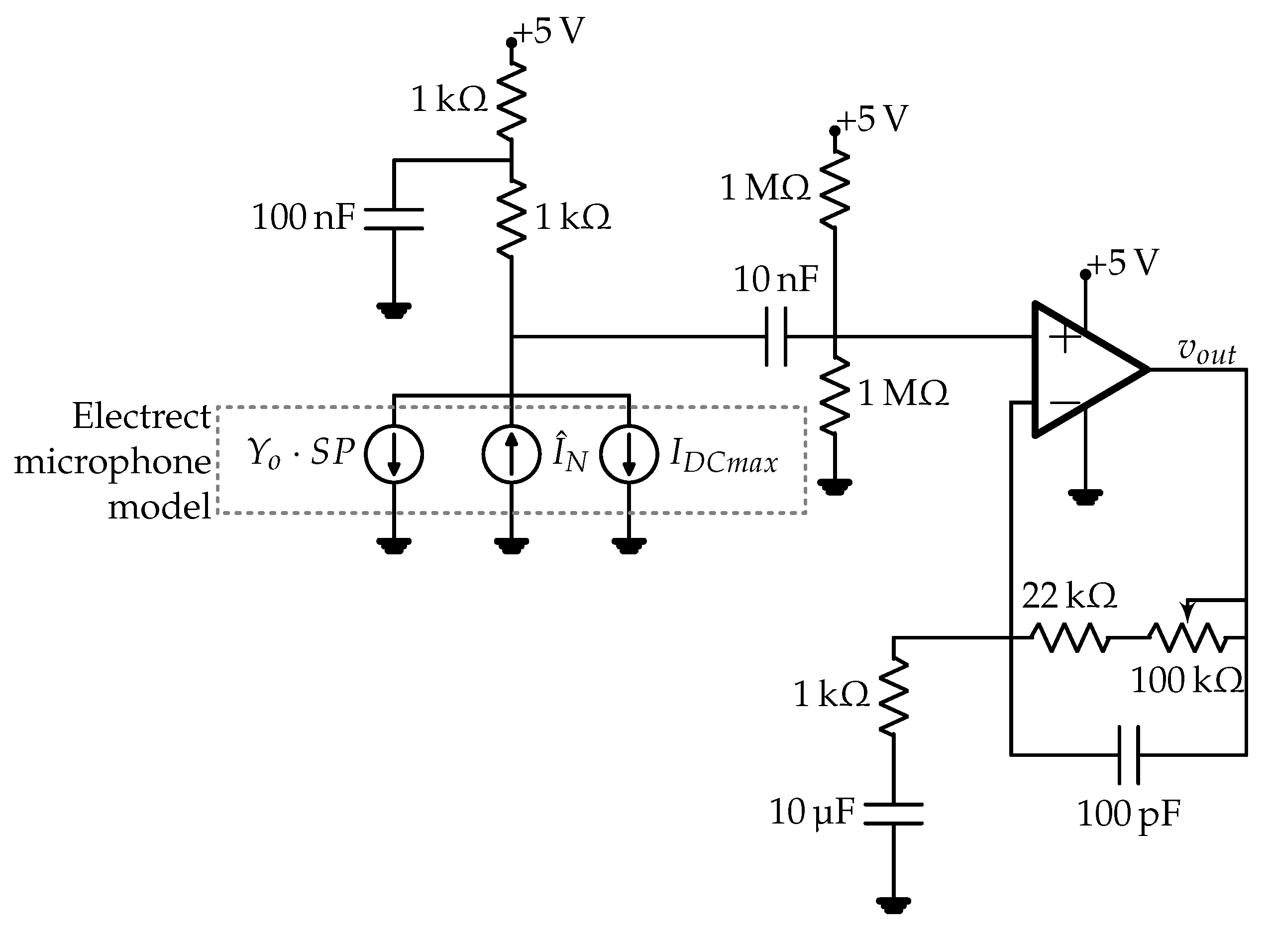
| Microphone | To measure the sound of the IVT. The selected microphone was an omnidirectional electret condenser microphone from CUI Inc. with a −44 dB sensitivity, an operating frequency in the range (0.02, 20) kHz. |
| PQA | To analyze current and voltage. |
| Line capacities | To model the line (from 1 to 50 µF) capacities and to generate different ferroresonance types. |
| Voltage source | To feed the IVT with AC voltage (4 kVA). |
| IVT | 220/:110/ V and 5 VA. |
| Switch stray capacity | To simulate the parasitic capacitance of grid switches. |
| Switches | To simulate the switches of the grid. |
| Isolation transformer | To make an isolated neutral system. |
| Value | NO | EFO | FO |
|---|---|---|---|
| 0.035 | 0.100 | 0.070 | |
| 0.047 | 0.559 | 0.099 |
| Accelerometer | Microphone | ||||||
|---|---|---|---|---|---|---|---|
| Test No. | Faulty | Close | Far | Inner | Inside | Outer | at |
| IVT | IVT | IVT | SG Panel | SG | SG Panel | 0.3 m | |
| # 1 | X | X | |||||
| # 2 | X | X | |||||
| # 3 | X | X | |||||
| # 4 | X | X | |||||
| # 5 | X | X | |||||
| # 6 | X | X | |||||
| Measured Parameter | Advantages | Disadvantages |
|---|---|---|
| Voltage waveforms | High accuracy in ferroresonance detection. | High sample rate and precision requirements. Isolation problems. High cost. |
| Temperature | Isolation problems. Low accuraccy in ferroresonance detection. | |
| Vibrations | Low cost. High accuracy in ferroresonance detection. | Isolation problems. Regular calibration. Accuracy sensitive to the installation procedures. |
| Acoustic Noise | Low cost. High accuracy in ferroresonance detection. Accuracy less sensitive to the installation procedures. No isolation problems. | Sensitive to the microphone location. |
Disclaimer/Publisher’s Note: The statements, opinions and data contained in all publications are solely those of the individual author(s) and contributor(s) and not of MDPI and/or the editor(s). MDPI and/or the editor(s) disclaim responsibility for any injury to people or property resulting from any ideas, methods, instructions or products referred to in the content. |
© 2022 by the authors. Licensee MDPI, Basel, Switzerland. This article is an open access article distributed under the terms and conditions of the Creative Commons Attribution (CC BY) license (https://creativecommons.org/licenses/by/4.0/).
Share and Cite
Martinez, R.; Arroyo, A.; Pigazo, A.; Manana, M.; Bayona, E.; Azcondo, F.J.; Bustamante, S.; Laso, A. Acoustic Noise-Based Detection of Ferroresonance Events in Isolated Neutral Power Systems with Inductive Voltage Transformers. Sensors 2023, 23, 195. https://doi.org/10.3390/s23010195
Martinez R, Arroyo A, Pigazo A, Manana M, Bayona E, Azcondo FJ, Bustamante S, Laso A. Acoustic Noise-Based Detection of Ferroresonance Events in Isolated Neutral Power Systems with Inductive Voltage Transformers. Sensors. 2023; 23(1):195. https://doi.org/10.3390/s23010195
Chicago/Turabian StyleMartinez, Raquel, Alberto Arroyo, Alberto Pigazo, Mario Manana, Eduardo Bayona, Francisco J. Azcondo, Sergio Bustamante, and Alberto Laso. 2023. "Acoustic Noise-Based Detection of Ferroresonance Events in Isolated Neutral Power Systems with Inductive Voltage Transformers" Sensors 23, no. 1: 195. https://doi.org/10.3390/s23010195