
PeakForce AFM Analysis Enhanced with Model Reduction Techniques


Abstract
:1. Introduction
- clustering analysis;
- manifold reparametrization.
2. Theoretical Background of the PeakForce-QNM Mode
3. Combined Proper Orthogonal Decomposition and Machine Learning Algorithm
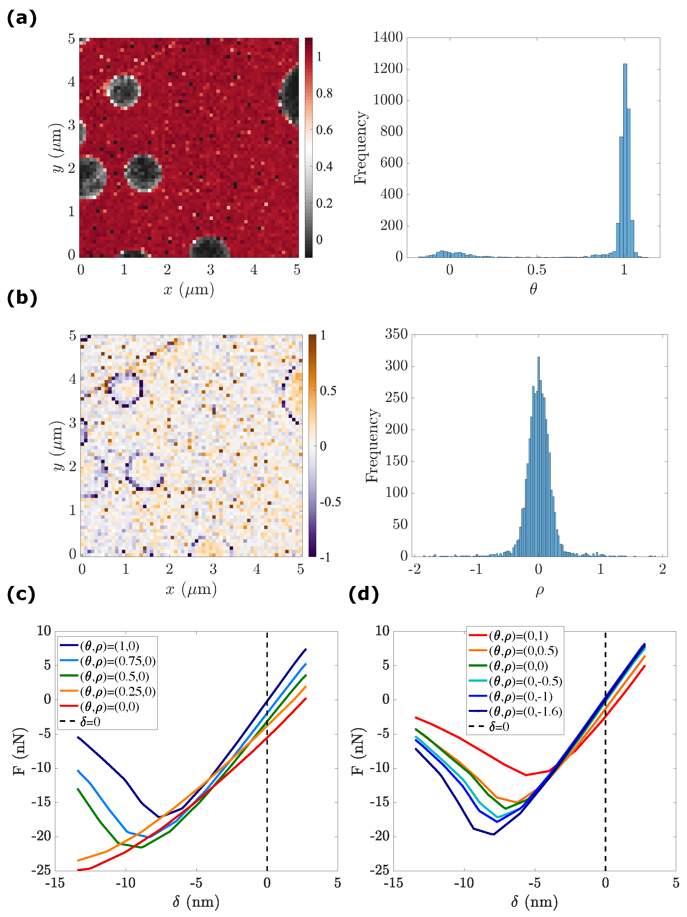
3.1. An Introductory Example about Pattern Recognition
- to segment any mechanically relevant phases;
- to identify the interface between each phase;
- to refine the segmentation if required, highlighting the contribution of higher-order parameters, such as topography variations.
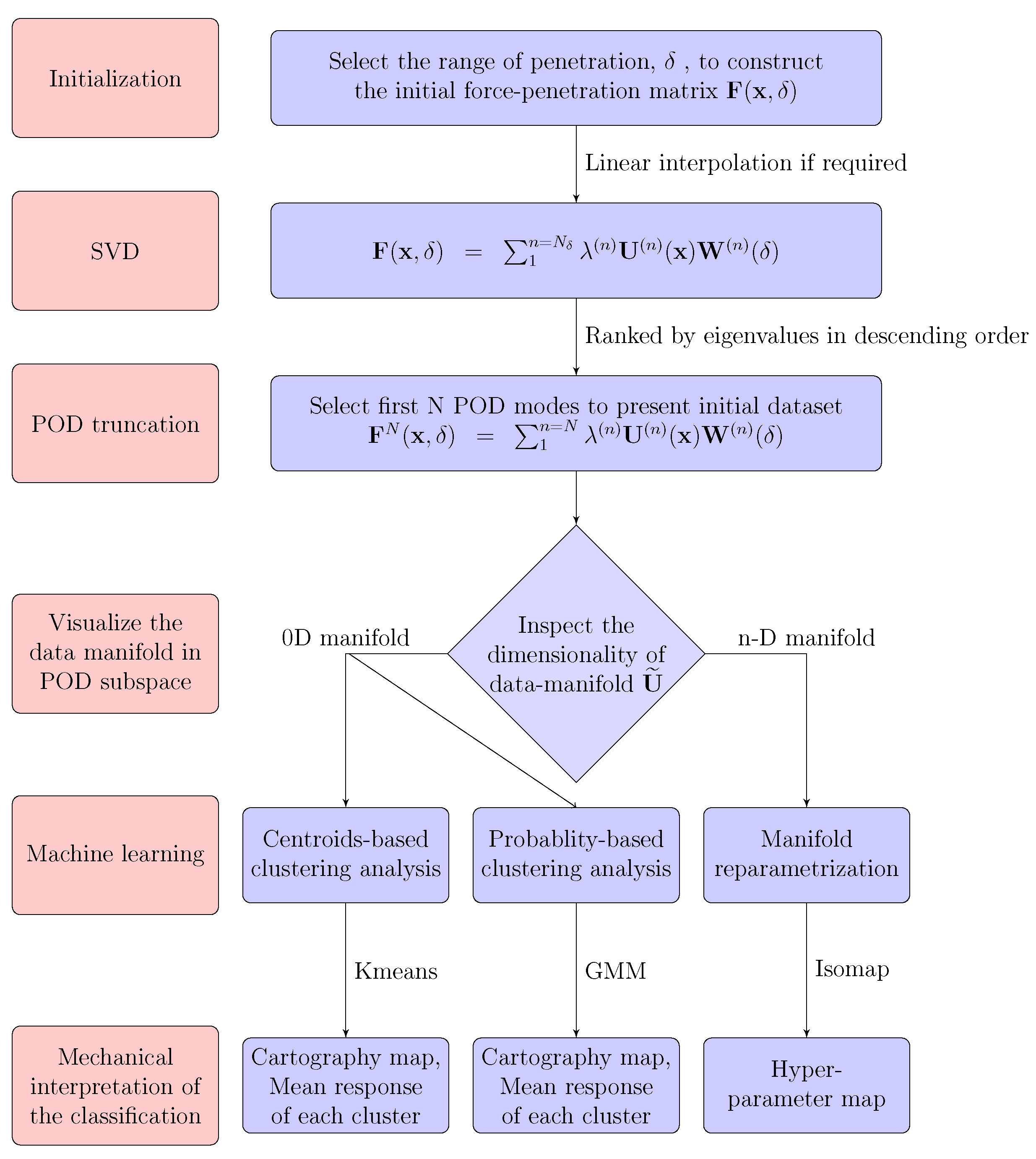
3.2. The General Framework of the POD-ML Combined Algorithm
- zero-dimensional manifolds: The data are grouped into several discrete clusters in the POD subspace. Clustering analysis is recommended in this case. K-means is the simplest choice, but requires good initialization. A probability-based clustering analysis, such as provided by the Gaussian mixture model (GMM), is an interesting alternative that gives additional information: not only centroids, but also statistical (co-)variance of each cluster.
- -dimensional manifold: One may propose an -coordinate manifold re-parameterization to smoothly interpolate between different responses.
4. Results and Discussion
4.1. Sample of PS-LDPE
4.1.1. Description of the Sample
4.1.2. POD Truncation
- τn:
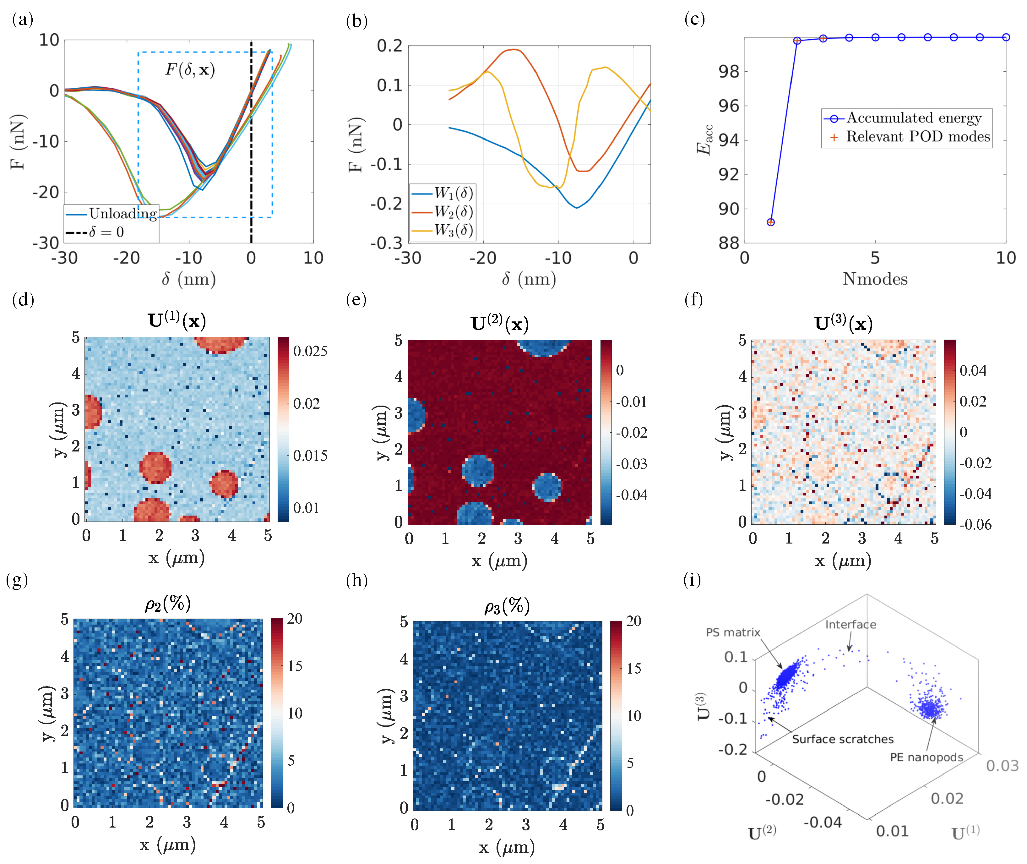
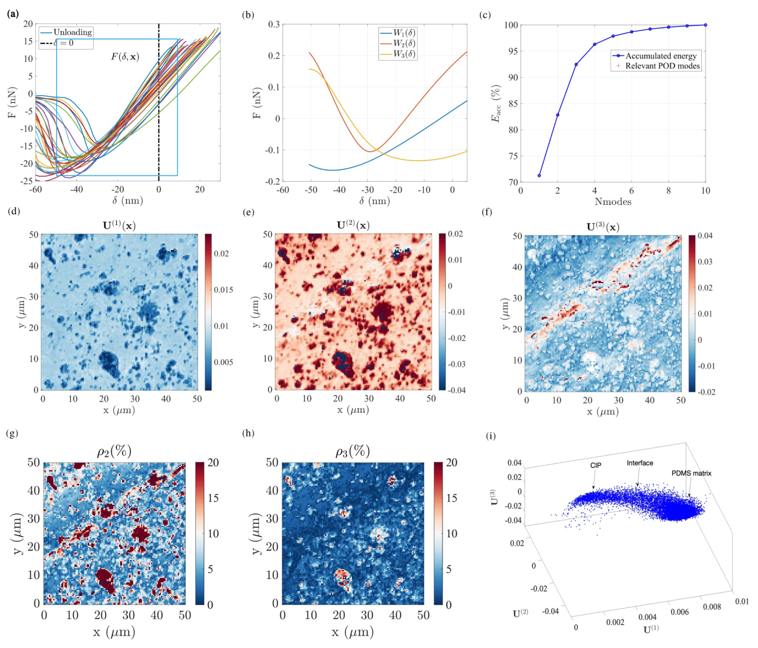
- the associated eigenvalue represents the power (in the sense of an L2 norm) of the -th POD mode in the total matrix. The accumulated power represents the total power contribution using the first POD modes to represent the entire dataset. In the case of PS–LDPE, the first three POD modes are chosen to represent the entire force–penetration evolution, which occupies the majority of the “energy” (L2-norm of the reconstructed signal after truncation compared to that of the raw data) contribution (up to 99%). Let us stress that the term “energy” here refers to a way to assess the fidelity of the captured signal after modal truncation, and not to a mechanical energy.
- U(1):
- the first POD mode contains the primary information on the phases. As shown in Figure 3d, the nature of each phase is remarkably well captured (PS in grey and LDPE in dark red).
- U(2):
- the second POD mode reveals the next-order information (e.g., phase interface). As illustrated in Figure 3e, the light grey areas at the PS–LPDE interfaces indicate that the mechanical properties at these pixels are somewhat different compared to either the PS matrix or the LDPE nanodisk.
- U(3):
- the third POD mode reveals even more subtle information that does not affect the first two POD modes. For instance, (as highlighted in Figure 3f) the map reveals regions with steep slopes, such as a scratch at the south-east side, which correlates well with similar defects revealed in SEM images. Moreover, also reveals the contact points of the AFM tip with the LDPE pods (Figure 3f), where the difference in the effective contact surface can be related to the observed behaviour at these pixels.
- ρ:
- the effect of higher-order POD modes, , has a negligible power. In this regard, the residual field, can be computed to locally evaluate the accuracy of POD reconstruction by using the first POD modes. In the presented case, if only the two first POD modes are used to reconstruct the force–penetration curve for the entire ROI, the residual field indicates a large reconstruction error up to 50%, particularly located in the region of LDPE nanopods. However, when using the first three POD modes, the reconstruction residual is significantly decreased to 8% on average, and no particular dependence is observed between the topography and residual field. A closer inspection shows that at the PS and LDPE interface, residuals remain high (about 5%), not higher than other points in the analysed region, but never small, so that the interface can still be perceived. This may result from the natural variability that is expected along the boundary of the pods both because of the different materials and the change in topography.
- Using the distribution of data in the subspace , Figure 3h shows that all pixels are grouped in different clusters.
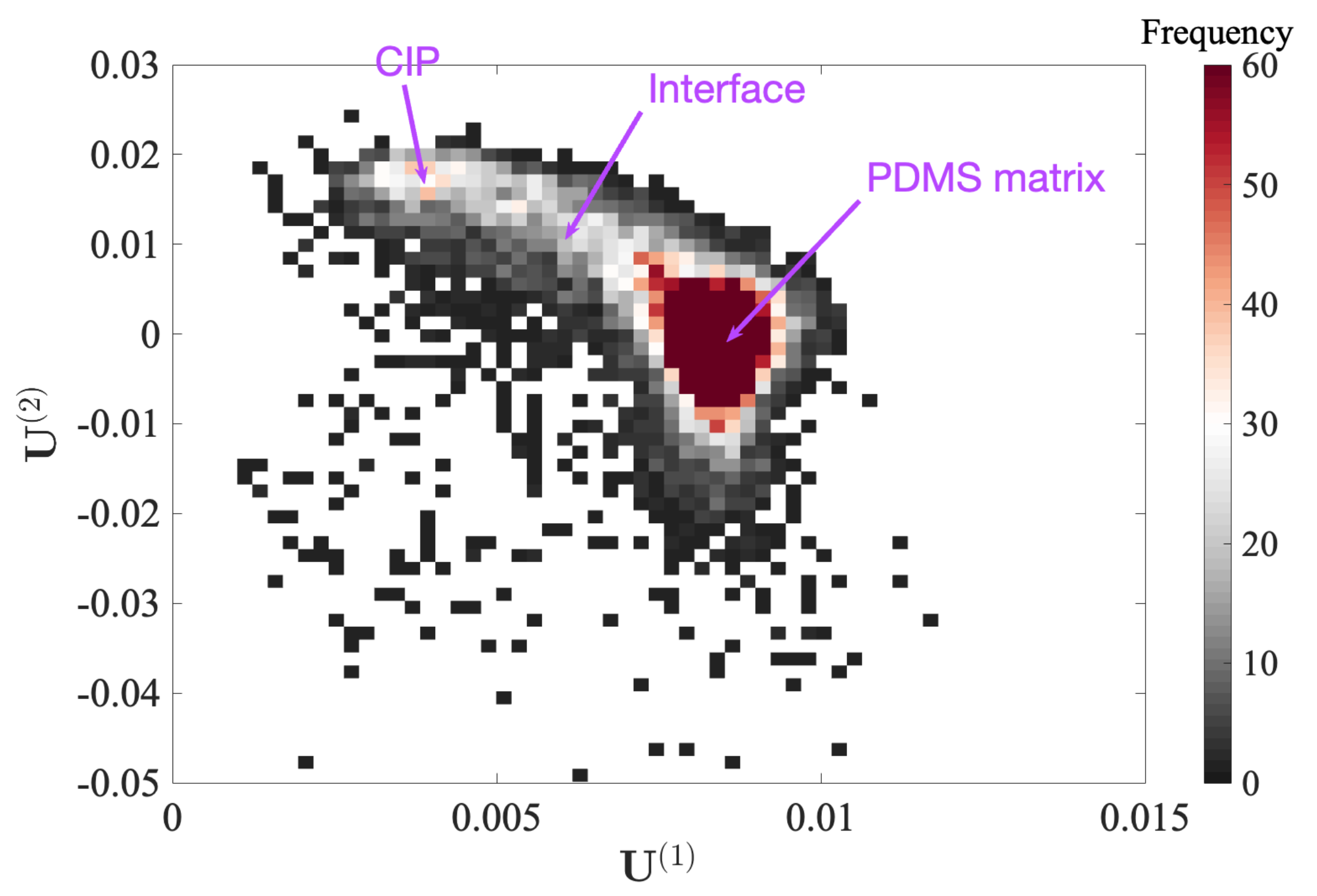
- Alternatively, using the first two modes, , a 2D histogram can be plotted [22], which shows the frequency of pixel distributions having a given value of and .
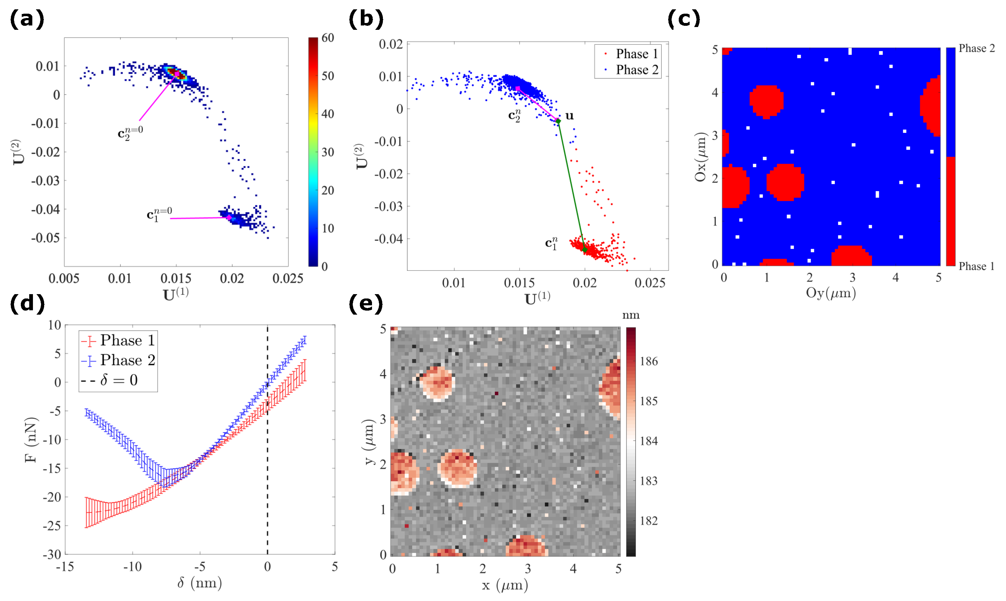
4.1.3. K-Means Clustering
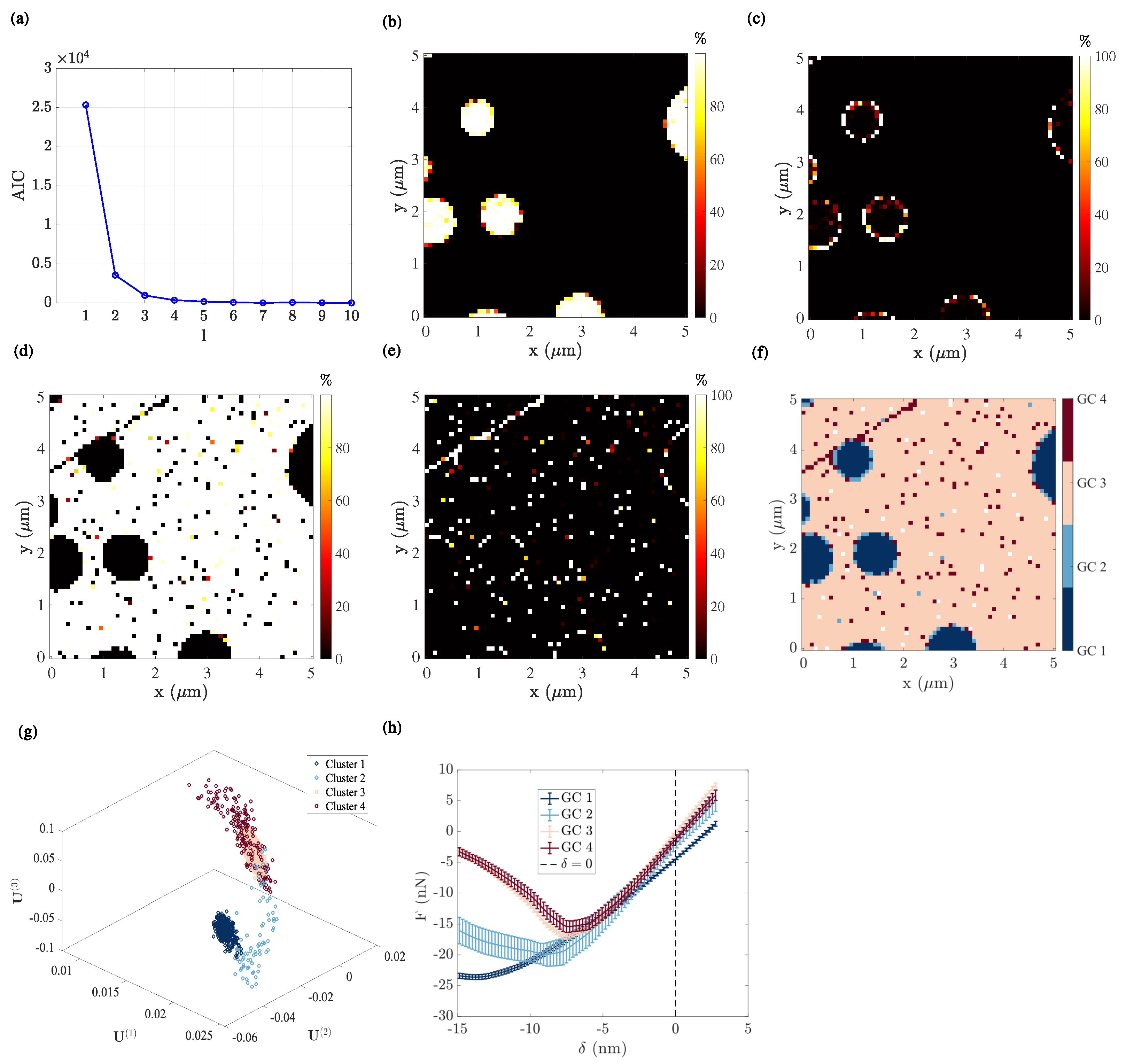
4.1.4. Gaussian Mixture Model
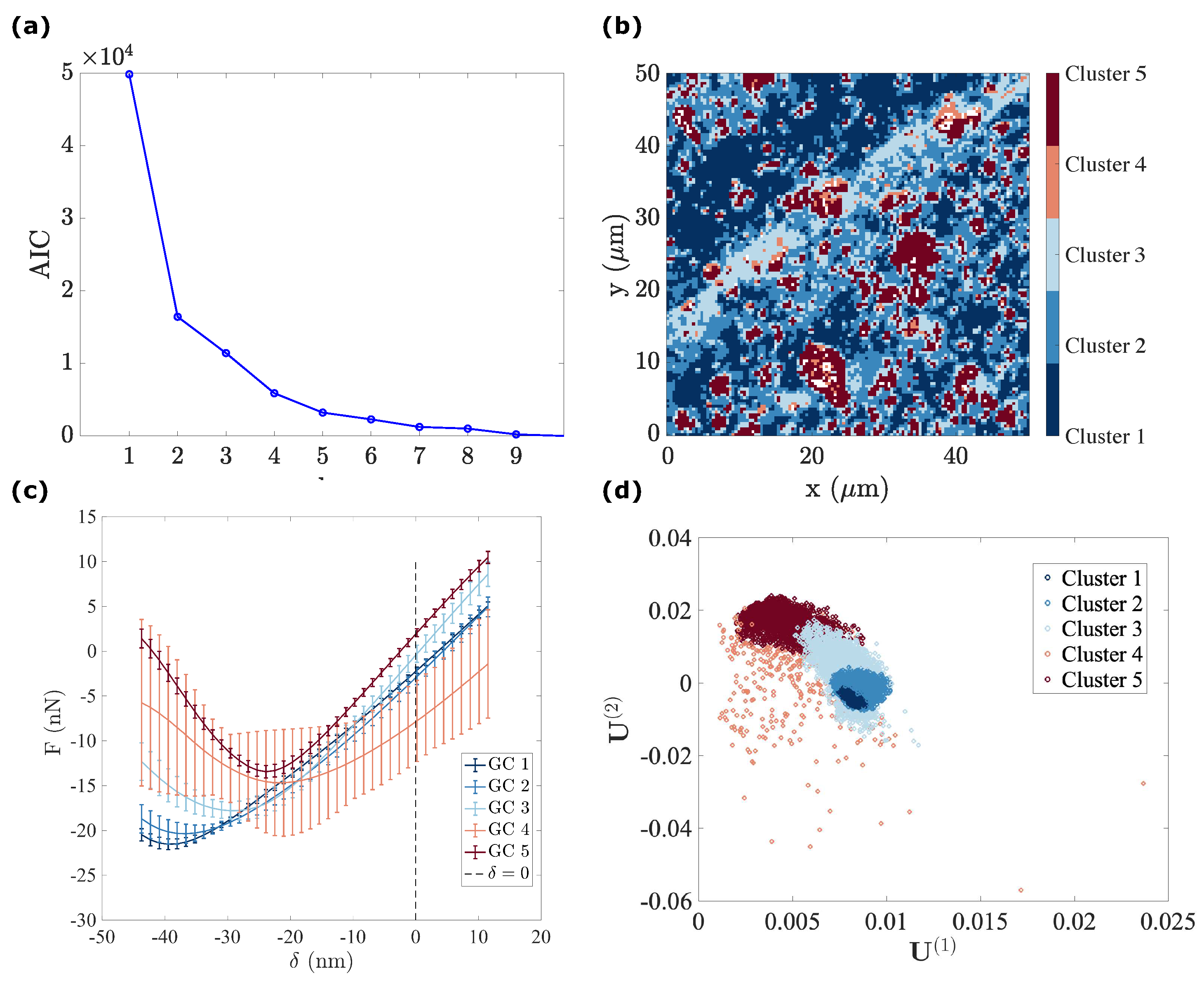
Number of Components
GMM Clustering Analysis
- (1)
- The first GC (Figure 5b) corresponds to the LDPE nanodisks, with a posterior probability very close to 1. Consistently, it exhibits the lowest force–indentation slope (highest compliance) among all clusters. Upon unloading, the position for which is the highest indicates a marked viscous behaviour (Figure 5h).
- (2)
- (3)
- (4)
- The fourth GC (Figure 5e) is more difficult to interpret. Indeed, it shows a mechanical response very similar to that of the third GC, and indeed in the space, these two components exhibit a wide overlap. The main difference comes from the much wider scatter of the fourth GC. This may be the result of the fact that the distribution of modal amplitudes for the PS film is not Gaussian. However, in the region where this component does not overlap with the third one, (well captured in the GC labelling), it highlights the topography contribution inside the PS film, revealing the presence of a surface defect (in particular, a scratch in the north-west corner). The underlying topography variation results in a larger scatter in terms of force indentation. It can then be concluded that sharp topography variations of the PS film, such as scratches, can be distinguished from the plain flat surface, mostly because of their scatter, and this subtle property is well captured by the GMM procedure.
4.1.5. Manifold Reparametrization
- corresponds to the LPDE phase (nanodisk deposit) with the lowest force–indentation slope and highest adhesion.
- corresponds to the PS phase (film matrix), with the highest stiffness and lowest adhesion.
- corresponds to the PS–LDPE interfaces, with an intermediate value of both stiffness and adhesion. As expected, with an increasing value of , we observe an increase in stiffness and a decrease in adhesion.
- For any given pixel , when is around zero (), the surface can be considered as smooth and when is shifting away from the mid-width of the Gaussian distribution (), the surface becomes rough (with significant topographical variations).
- Interestingly, different types of topographical features are associated with different values of , i.e.,
- –
- surface defects (scratch): ;
- –
- phase interface (frontal interface between the LDPE nanodisk and AFM tip): .
4.2. Carbon–Iron Particles with a PDMS Binder
4.2.1. Gaussian Mixture Model Fitting
- GC 1, 2 and 3 (PDMS matrix): the first three components plotted in dark, medium and light blue represent the majority of the PDMS matrix with a very comparable soft modulus and small viscosity. Their adhesion tends to decrease from GC 1 to GC 3. Moreover, the spatial distribution of the components suggests that the main difference between these three components is due to topography, from a plateau level for GC 1, down to deep valleys (scratches) for GC 3. This observation may be due to the maximum penetration being high for GC 1 and low for GC 3, and the effectively mobilized adhesion may be due to the indentation depth.
- GC 4 (PDMS–CIP interface): as illustrated in Figure 10d, most of the data points that belong to the forth cluster are very widely scattered, and hence they may be difficult to interpret. However, their location is clearly in very close vicinity to the CIP or CIP aggregates. The most salient feature of their mechanical response (apart from the expected broad dispersion) is their high viscosity. This may result from the enhanced strain and strain rates in the PDMS phase when it is confined within a CIP cluster, resulting in an amplification of the viscous contribution.
- GC 5 (CIP): The fifth component (plotted in dark red) exhibits the highest force–indentation slope, low adhesion, and low viscosity. This observation is consistent with their morphology, supporting the fact that it corresponds to CIPs at the surface.
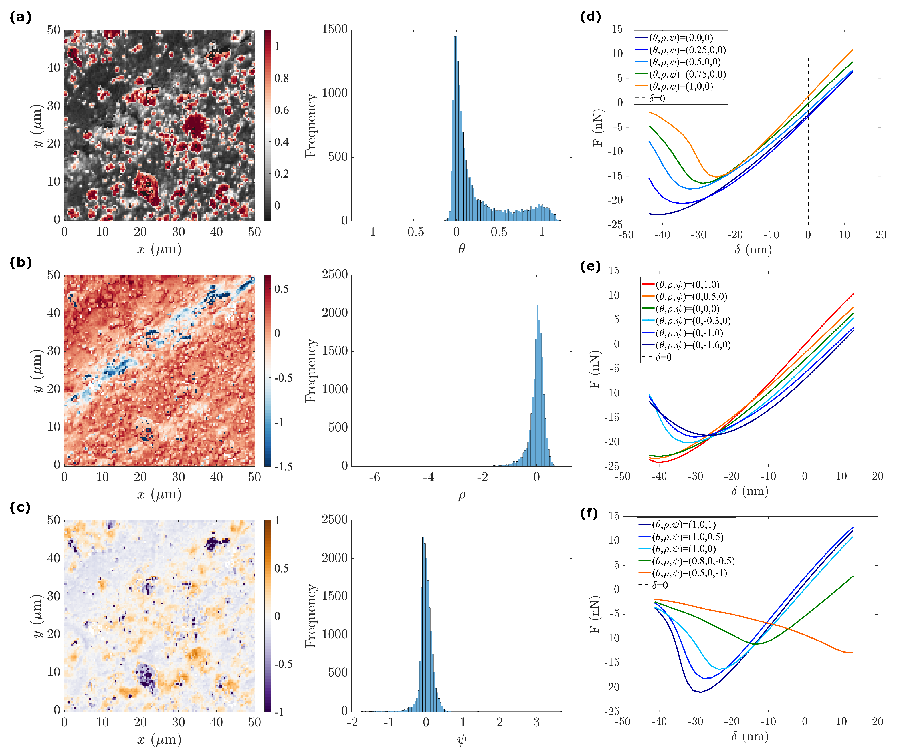
4.2.2. Manifold Re-Parametrization
- : We study the effect by setting to their mean value , respectively. By varying the first state variable (), we observe a progressive increase in the stiffness ( slope) and a decrease in adhesion (see Figure 11e). The response of exhibits the highest force–indentation slope, a near-zero dissipation, and the lowest adhesion, corresponding to the presence of CIPs. The response of shows the lowest apparent modulus and highest adhesion, corresponding to the presence of a viscous and adhesive PDMS matrix. As for all intermediate values, , the corresponding response indicates a progressive evolution, especially in adhesion, implying a decrease in the influence of the PDMS matrix as increases.
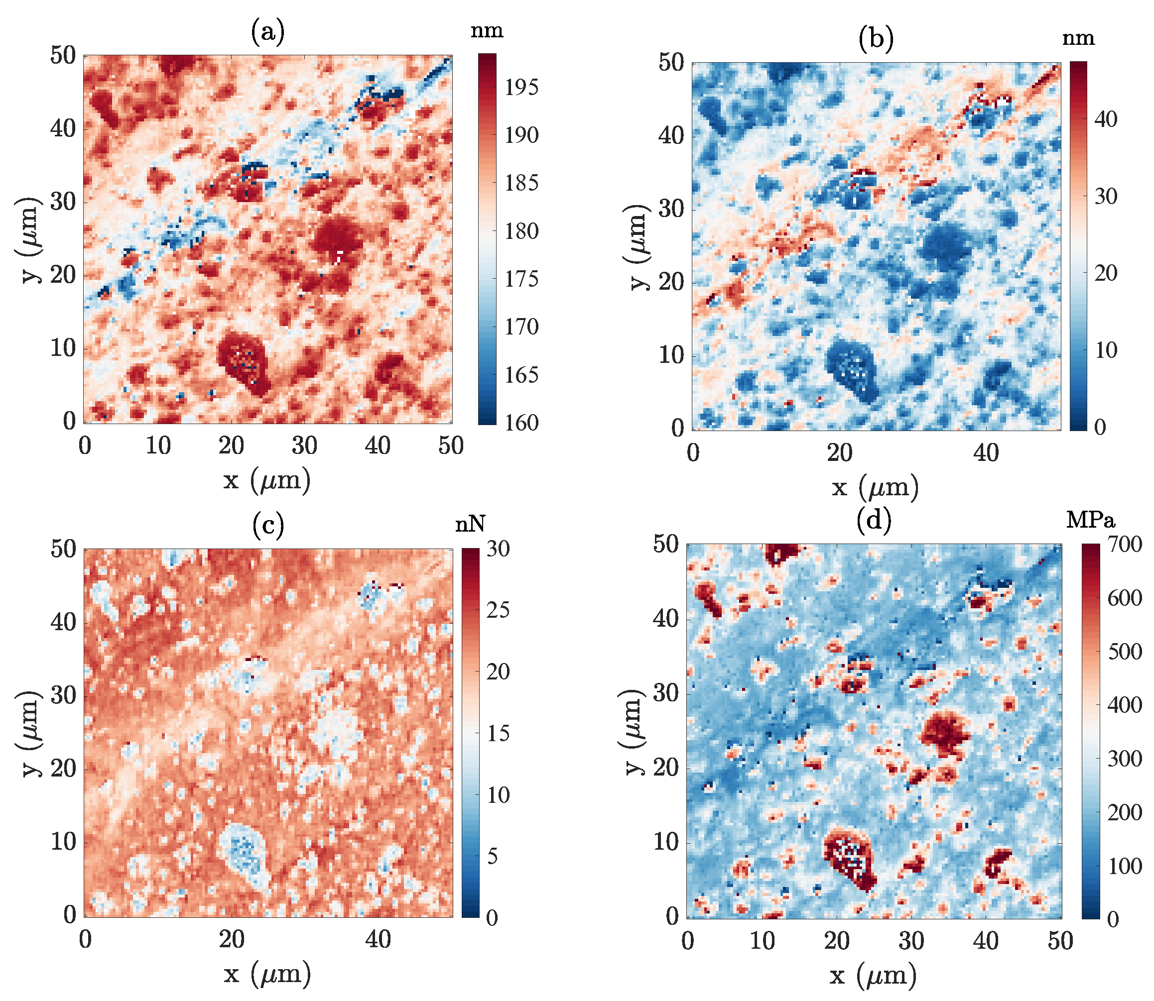
- : The second state variable map, , (Figure 11b) correlates well with surface topography (Figure 8c). From deep in the valley where , the mean surface , and to the most salient peaks where , the surface topography becomes the main characteristic captured by . Force indentation responses with different values of (see Figure 11e) were compared by setting the two other state variables to 0 (focusing mainly on the PDMS matrix). Compared to the standard PDMS matrix surface, , the force–indentation response in the valley, where , leads to a significant decrease in the apparent adhesion while maintaining a similar stiffness. This observation is consistent with previous observations of the GMM analysis, where it was argued that for deep valleys, the penetration distance and effective contact radius is somewhat smaller than for higher regions, and hence the apparent adhesion is expected to be reduced.Furthermore, focusing on the deepest positions inside the valley ( varying from to ), an increasing viscosity is observed. This increasing viscosity can be interpreted as an artefact due to the tip velocity. Note that for a local scan inside a deep valley where the topography is much lower than the average surface (see Figure 8d), the tip should be subjected to an increased velocity to comply with the required AFM scanning frequency at . To further support this interpretation, Figure 8d shows that the largest penetration distances (excluded from the analysis because of our selected range of ) are associated with the largest apparent viscosity values. On the contrary, when is positive () the force–indentation response shows a similar adhesion to a plain PDMS surface with increased stiffness, implying the presence of CIPs buried just below the PDMS surface. Therefore, the map reveals the impact of surface topography on the mechanical response (and in some respect also on the acquisition artefacts).
- : The distribution of follows a single peak distribution. For this state variable, values very different from 0 are mostly concentrated in large CIPs or CIP aggregates. Thus, in setting , the main effect of increasing from zero is a significant variation in adhesion. This may be interpreted as the effect of either particle immersion or being covered by a thin layer of PDMS that changes the adhesion by a large amount without altering stiffness (over the penetration range).Large negative values (purple-blue in Figure 11c) correspond with pixels located either very deep in the valley or very high at salient peaks. They also coincide with regions where . When compared to the previous analyses, all these pixels correspond to the fourth GC, and in terms of modes, they could be identified in modes 1 and 2 as data points that do not exhibit smooth continuity with their surrounding. When the force–displacement response is computed for two sets of values and , as shown in Figure 11f), odd non-physical shapes are obtained. All these observations support the fact that these measurements were unreliable, as previously observed, and when forced to organize these data in a sensible way, very unusual values and increased scattering of the various properties may be obtained. In this view, the obtained range of values for mainly show pixels that should be discarded rather than providing a trustworthy measurement of a given mechanical quantity.
5. Conclusions
Author Contributions
Funding
Institutional Review Board Statement
Informed Consent Statement
Data Availability Statement
Acknowledgments
Conflicts of Interest
References
- Zhao, M.; Lu, Q.; Ma, Q.; Zhang, H. Two-dimensional metal–organic framework nanosheets. Small Methods 2017, 1, 1600030. [Google Scholar] [CrossRef]
- Nievergelt, A.P.; Kammer, C.; Brillard, C.; Kurisinkal, E.; Bastings, M.M.C.; Karimi, A.; Fantner, G.E. Large-Range HS-AFM Imaging of DNA Self-Assembly through in Situ Data-Driven Control. Small Methods 2019, 3, 1900031. [Google Scholar] [CrossRef]
- Binnig, G.; Quate, C.F.; Gerber, C. Atomic Force Microscope. Phys. Rev. Lett. 1986, 56, 930–933. [Google Scholar] [CrossRef] [PubMed]
- Magonov, S.; Elings, V.; Whangbo, M.H. Phase imaging and stiffness in tapping-mode atomic force microscopy. Surf. Sci. 1997, 375, L385–L391. [Google Scholar] [CrossRef]
- Rosa-Zeiser, A.; Weilandt, E.; Hild, S.; Marti, O. The simultaneous measurement of elastic, electrostatic and adhesive properties by scanning force microscopy: Pulsed-force mode operation. Meas. Sci. Technol. 1997, 8, 1333–1338. [Google Scholar] [CrossRef]
- Passeri, D.; Rossi, M.; Vlassak, J. On the tip calibration for accurate modulus measurement by contact resonance atomic force microscopy. Ultramicroscopy 2013, 128, 32–41. [Google Scholar] [CrossRef]
- Garcia, R.; Perez, R. Dynamic atomic force microscopy methods. Surf. Sci. Rep. 2002, 47, 197–301. [Google Scholar] [CrossRef]
- Young, T.J.; Monclus, M.A.; Burnett, T.L.; Broughton, W.R.; Ogin, S.L.; Smith, P.A. The use of the PeakForceTMquantitative nanomechanical mapping AFM-based method for high-resolution Young’s modulus measurement of polymers. Meas. Sci. Technol. 2011, 22, 125703. [Google Scholar] [CrossRef]
- Sweers, K.K.M.; van der Werf, K.O.; Bennink, M.L.; Subramaniam, V. Atomic Force Microscopy under Controlled Conditions Reveals Structure of C-Terminal Region of α-Synuclein in Amyloid Fibrils. ACS Nano 2012, 6, 5952–5960. [Google Scholar] [CrossRef]
- Dokukin, M.E.; Sokolov, I. Quantitative Mapping of the Elastic Modulus of Soft Materials with HarmoniX and PeakForce QNM AFM Modes. Langmuir 2012, 28, 16060–16071. [Google Scholar] [CrossRef]
- Pfreundschuh, M.; Alsteens, D.; Hilbert, M.; Steinmetz, M.O.; Müller, D.J. Localizing Chemical Groups while Imaging Single Native Proteins by High-Resolution Atomic Force Microscopy. Nano Lett. 2014, 14, 2957–2964. [Google Scholar] [CrossRef] [PubMed]
- Liao, H.S.; Lei, K.K.; Tseng, Y.F. High-speed force mapping based on an astigmatic atomic force microscope. Meas. Sci. Technol. 2019, 30, 027002. [Google Scholar] [CrossRef]
- Barthel, E.; Roux, S. Velocity-Dependent Adherence: An Analytical Approach for the JKR and DMT Models. Langmuir 2000, 16, 8134–8138. [Google Scholar] [CrossRef]
- Jay, G.D.; Torres, J.R.; Rhee, D.K.; Helminen, H.J.; Hytinnen, M.M.; Cha, C.J.; Elsaid, K.; Kim, K.S.; Cui, Y.; Warman, M.L. Association between friction and wear in diarthrodial joints lacking lubricin. Arthritis Rheum. 2007, 56, 3662–3669. [Google Scholar] [CrossRef] [PubMed]
- Li, Q.; Kim, K.S. Micromechanics of friction: Effects of nanometre-scale roughness. Proc. R. Soc. A Math. Phys. Eng. Sci. 2008, 464, 1319–1343. [Google Scholar] [CrossRef]
- Lin, D.; Dimitriadis, E.; Horkay, F. Robust Strategies for Automated AFM Force Curve Analysis—I. Non-adhesive Indentation of Soft, Inhomogeneous Materials. J. Biomech. Eng. 2007, 129, 430–440. [Google Scholar] [CrossRef]
- Lin, D.; Dimitriadis, E.; Horkay, F. Robust Strategies for Automated AFM Force Curve Analysis—II: Adhesion-Influenced Indentation of Soft, Elastic Materials. J. Biomech. Eng. 2008, 129, 904–912. [Google Scholar] [CrossRef]
- Briscoe, B.J.; Fiori, L.; Pelillo, E. Nano-indentation of polymeric surfaces. J. Phys. D Appl. Phys. 1998, 31, 2395–2405. [Google Scholar] [CrossRef]
- Kassa, H.G.; Stuyver, J.; Bons, A.J.; Haviland, D.B.; Thorén, P.A.; Borgani, R.; Forchheimer, D.; Leclère, P. Nano-mechanical properties of interphases in dynamically vulcanized thermoplastic alloy. Polymer 2018, 135, 348–354. [Google Scholar] [CrossRef]
- Petrov, M.; Sokolov, I. Identification of Geometrical Features of Cell Surface Responsible for Cancer Aggressiveness: Machine Learning Analysis of Atomic Force Microscopy Images of Human Colorectal Epithelial Cells. Biomedicines 2023, 11, 191. [Google Scholar] [CrossRef]
- Verleysen, M.; François, D. The Curse of Dimensionality in Data Mining and Time Series Prediction. In Proceedings of the Computational Intelligence and Bioinspired Systems: 8th International Work-Conference on Artificial Neural Networks, IWANN 2005, Vilanova i la Geltrú, Barcelona, Spain, 8–10 June 2005; Volume 3512, pp. 758–770. [Google Scholar] [CrossRef]
- Chang, X.; Hallais, S.; Roux, S.; Danas, K. Model reduction techniques for quantitative nano-mechanical AFM mode. Meas. Sci. Technol. 2021, 32, 075406. [Google Scholar] [CrossRef]
- Chatterjee, A. An introduction to the proper orthogonal decomposition. Curr. Sci. 2000, 78, 808–817. [Google Scholar]
- Van Loan, C.F. Generalizing the singular value decomposition. SIAM J. Numer. Anal. 1976, 13, 76–83. [Google Scholar] [CrossRef]
- Wold, S.; Esbensen, K.; Geladi, P. Principal component analysis. Chemom. Intell. Lab. Syst. 1987, 2, 37–52. [Google Scholar] [CrossRef]
- Ranti, D.; Warburton, A.J.; Hanss, K.; Katz, D.; Poeran, J.; Moucha, C. K-Means Clustering to Elucidate Vulnerable Subpopulations among Medicare Patients Undergoing Total Joint Arthroplasty. J. Arthroplast. 2020, 35, 3488–3497. [Google Scholar] [CrossRef]
- Singh, M.; Venkatesh, V.; Verma, A.; Sharma, N. Segmentation of MRI data using multi-objective antlion based improved fuzzy c-means. Biocybern. Biomed. Eng. 2020, 40, 1250–1266. [Google Scholar] [CrossRef]
- Su, M.S.; Chia, C.C.; Chen, C.Y.; Chen, J.F. Classification of partial discharge events in GILBS using probabilistic neural networks and the fuzzy c-means clustering approach. Int. J. Electr. Power Energy Syst. 2014, 61, 173–179. [Google Scholar] [CrossRef]
- Pyun, K.; Lim, J.; Won, C.S.; Gray, R.M. Image segmentation using hidden Markov Gauss mixture models. IEEE Trans. Image Process. 2007, 16, 1902–1911. [Google Scholar] [CrossRef]
- Cayton, L. Algorithms for manifold learning. Univ. Calif. San Diego Technol. Rep. 2005, 12, 1. [Google Scholar]
- Psarra, E.; Bodelot, L.; Danas, K. Two-field surface pattern control via marginally stable magnetorheological elastomers. Soft Matter 2017, 13, 6576–6584. [Google Scholar] [CrossRef]
- Mukherjee, D.; Rambausek, M.; Danas, K. An explicit dissipative model for isotropic hard magnetorheological elastomers. J. Mech. Phys. Solids 2021, 151, 104361. [Google Scholar] [CrossRef]
- Cappella, B.; Dietler, G. Force-distance curves by atomic force microscopy. Surf. Sci. Rep. 1999, 34, 1–104. [Google Scholar] [CrossRef]
- Rützel, S.; Lee, S.I.; Raman, A. Nonlinear dynamics of atomic force microscope probes driven in Lennard Jones potentials. Proc. R. Soc. Lond. Ser. A Math. Phys. Eng. Sci. 2003, 459, 1925–1948. [Google Scholar] [CrossRef]
- Muller, V.; Derjaguin, B.; Toporov, Y.P. On two methods of calculation of the force of sticking of an elastic sphere to a rigid plane. Colloids Surfaces 1983, 7, 251–259. [Google Scholar] [CrossRef]
- Bodelot, L.; Voropaieff, J.P.; Pössinger, T. Experimental investigation of the coupled magneto-mechanical response in magnetorheological elastomers. Exp. Mech. 2017, 58, 207–221. [Google Scholar] [CrossRef]
- Psarra, E.; Bodelot, L.; Danas, K. Wrinkling to crinkling transitions and curvature localization in a magnetoelastic film bonded to a non-magnetic substrate. J. Mech. Phys. Solids 2019, 133, 103734. [Google Scholar] [CrossRef]
- Moreno-Mateos, M.A.; Gonzalez-Rico, J.; Nunez-Sardinha, E.; Gomez-Cruz, C.; Lopez-Donaire, M.L.; Lucarini, S.; Arias, A.; Muñoz-Barrutia, A.; Velasco, D.; Garcia-Gonzalez, D. Magneto-mechanical system to reproduce and quantify complex strain patterns in biological materials. Appl. Mater. Today 2022, 27, 101437. [Google Scholar] [CrossRef]
- Moreno, M.; Gonzalez-Rico, J.; Lopez-Donaire, M.; Arias, A.; Garcia-Gonzalez, D. New experimental insights into magneto-mechanical rate dependences of magnetorheological elastomers. Compos. Part B Eng. 2021, 224, 109148. [Google Scholar] [CrossRef]
- Rambausek, M.; Mukherjee, D.; Danas, K. A computational framework for magnetically hard and soft viscoelastic magnetorheological elastomers. Comput. Methods Appl. Mech. Eng. 2022, 391, 114500. [Google Scholar] [CrossRef]
- Stifter, T.; Weilandt, E.; Marti, O.; Hild, S. Influence of the topography on adhesion measured by SFM. Appl. Phys. A 1998, 66, S597–S605. [Google Scholar] [CrossRef]


Disclaimer/Publisher’s Note: The statements, opinions and data contained in all publications are solely those of the individual author(s) and contributor(s) and not of MDPI and/or the editor(s). MDPI and/or the editor(s) disclaim responsibility for any injury to people or property resulting from any ideas, methods, instructions or products referred to in the content. |
© 2023 by the authors. Licensee MDPI, Basel, Switzerland. This article is an open access article distributed under the terms and conditions of the Creative Commons Attribution (CC BY) license (https://creativecommons.org/licenses/by/4.0/).
Share and Cite
Chang, X.; Hallais, S.; Danas, K.; Roux, S. PeakForce AFM Analysis Enhanced with Model Reduction Techniques. Sensors 2023, 23, 4730. https://doi.org/10.3390/s23104730
Chang X, Hallais S, Danas K, Roux S. PeakForce AFM Analysis Enhanced with Model Reduction Techniques. Sensors. 2023; 23(10):4730. https://doi.org/10.3390/s23104730
Chicago/Turabian StyleChang, Xuyang, Simon Hallais, Kostas Danas, and Stéphane Roux. 2023. "PeakForce AFM Analysis Enhanced with Model Reduction Techniques" Sensors 23, no. 10: 4730. https://doi.org/10.3390/s23104730
APA StyleChang, X., Hallais, S., Danas, K., & Roux, S. (2023). PeakForce AFM Analysis Enhanced with Model Reduction Techniques. Sensors, 23(10), 4730. https://doi.org/10.3390/s23104730