
A Millimeter-Wave 3D Imaging Algorithm for MIMO Synthetic Aperture Radar


Abstract
:1. Introduction
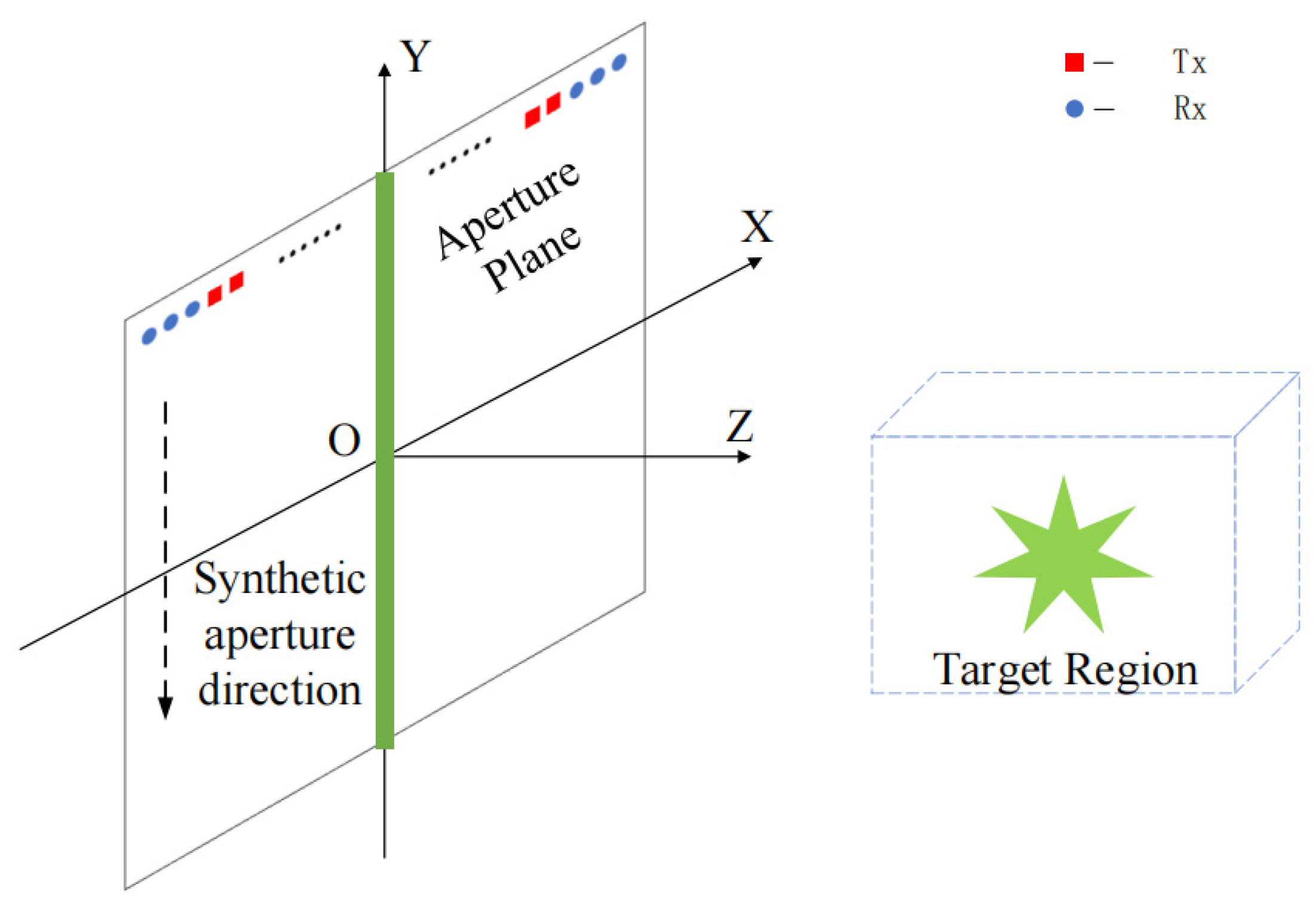
2. Formulation
2.1. Traditional BP Algorithm for MIMO-SAR Imaging
2.2. The Proposed Algorithm
2.3. The CF-Proposed Algorithm
2.4. Computation Complexity
2.5. Error Analysis
3. Numerical Simulation and Experimental Verification
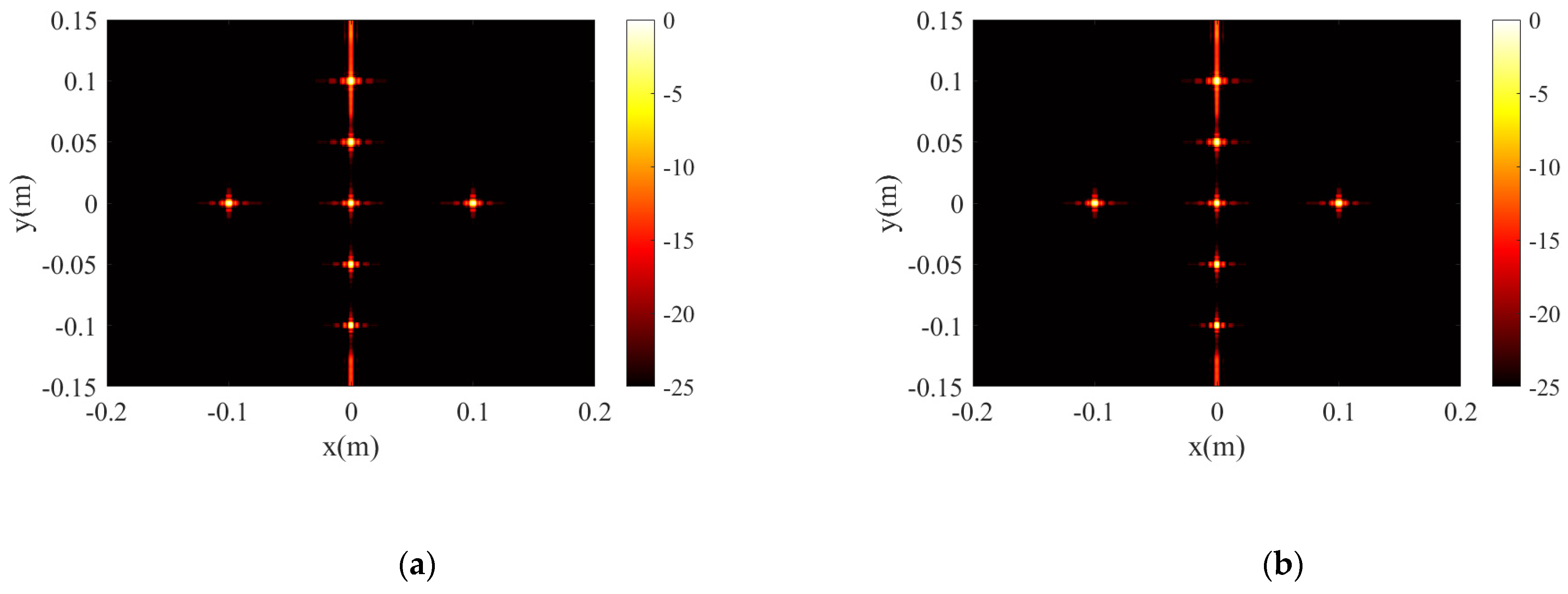
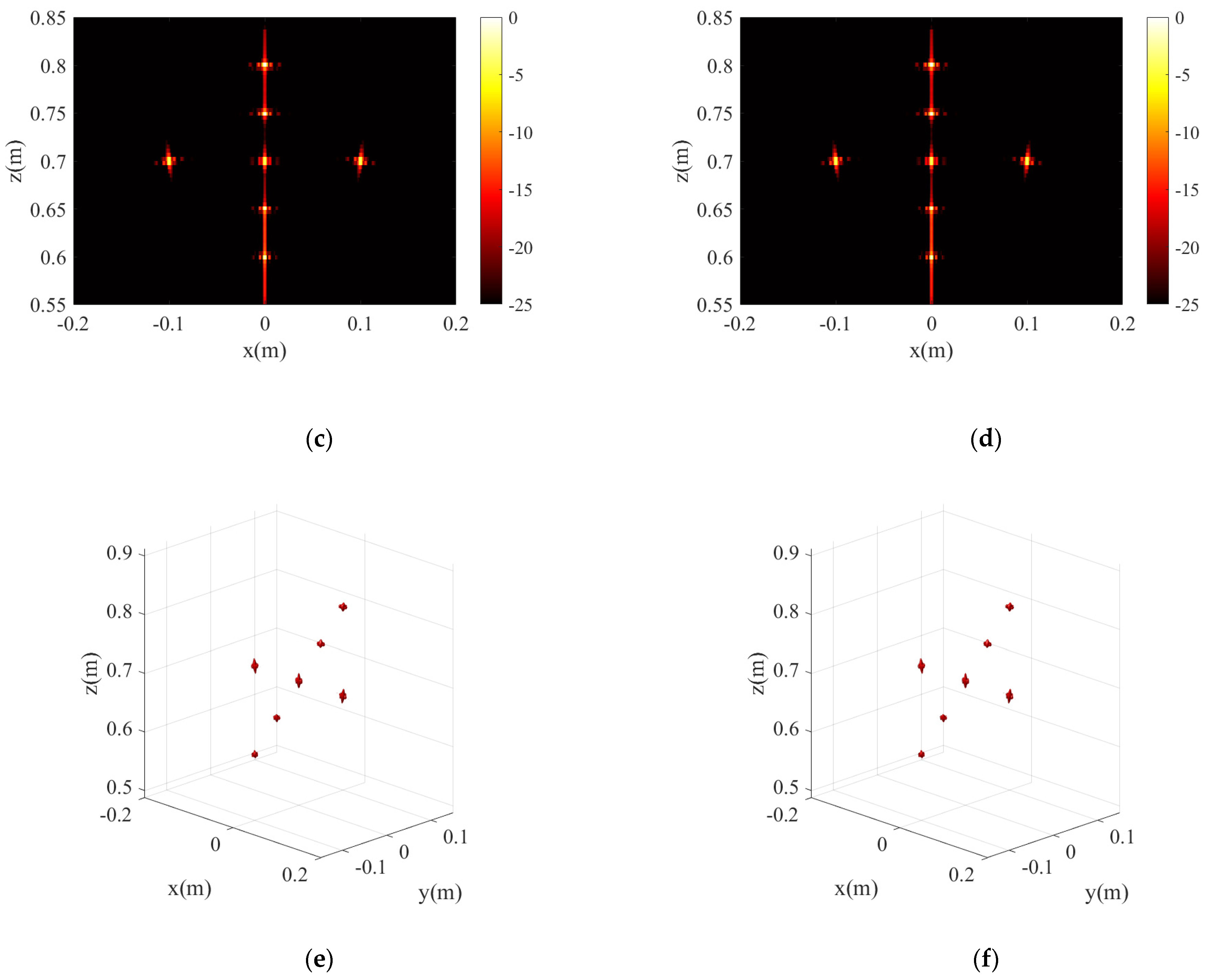
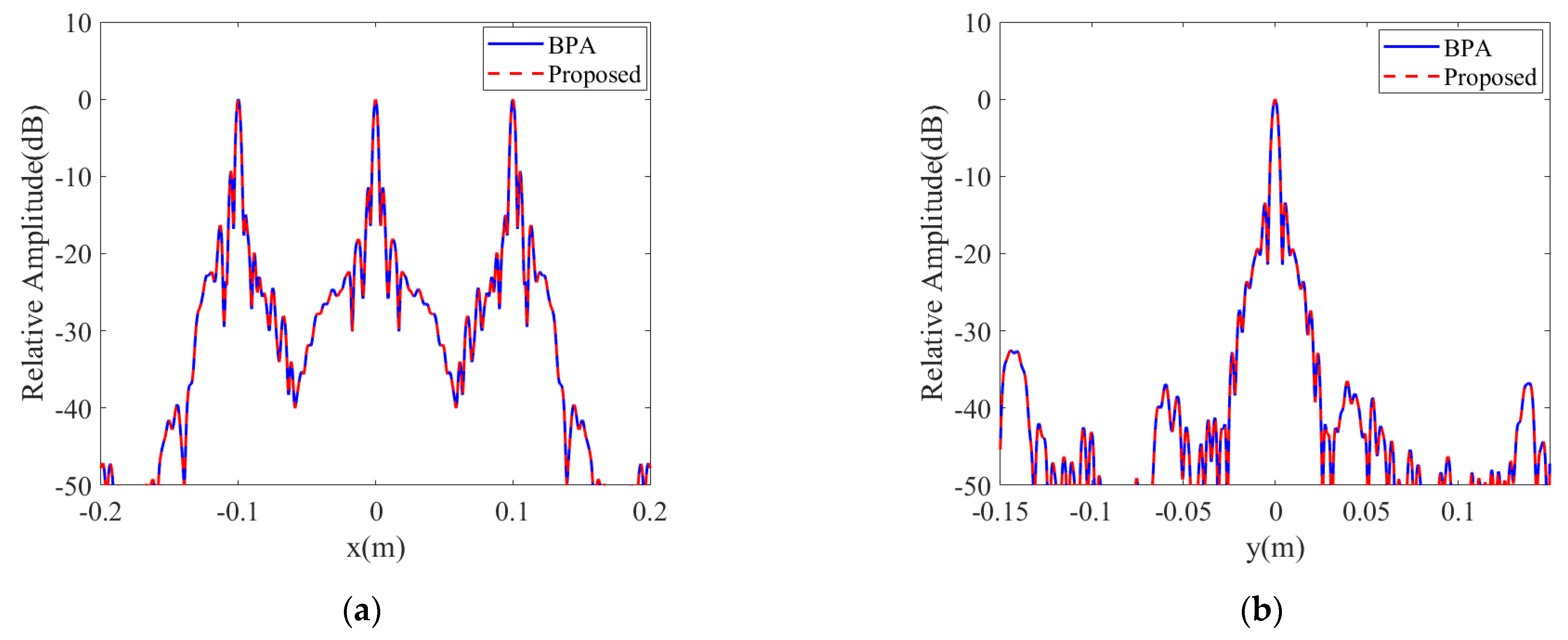
3.1. Simulation Results of Point Targets
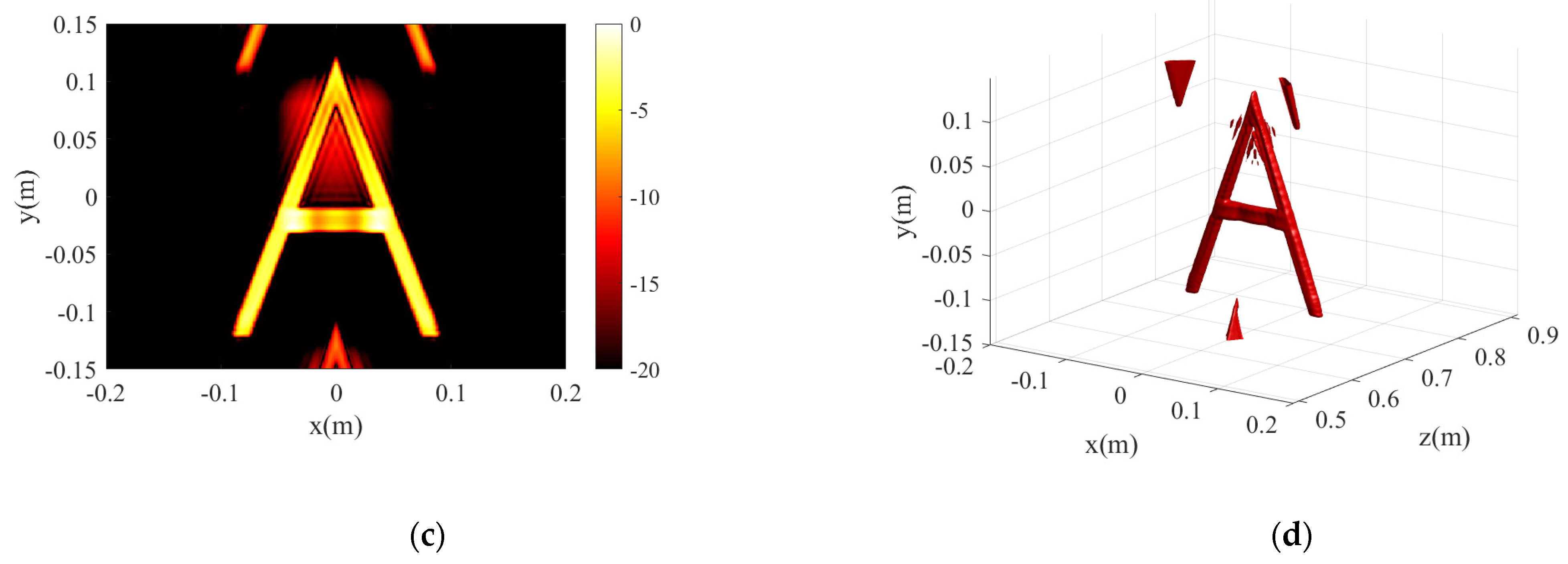
3.2. Simulation Results of Letter A Scattering Models
4. Lab Experiments Results
4.1. Lab Experiment 1
4.2. Lab Sparse Experiment 2
5. Discussion
6. Conclusions
Author Contributions
Funding
Data Availability Statement
Acknowledgments
Conflicts of Interest
References
- Zamani, H.; Fakharzadeh, M. 1.5-D sparse array for millimeter wave imaging based on compressive sensing techniques. IEEE Trans. Antennas Propag. 2018, 4, 2008–2015. [Google Scholar] [CrossRef]
- Heimbeck, M.S.; Kim, M.K.; Gregory, D.A.; Everitt, H.O. Terahertzdigital off-axis holography for non-destructive testing. In Proceedings of the International Conference on Infrared, Millimeter, and Terahertz Waves, Houston, TX, USA, 2–7 October 2011; Volume 10, pp. 1–2. [Google Scholar]
- Cheng, B.; Cui, Z.; Lu, B.; Qin, Y.; Liu, Q.; Chen, P.; He, Y.; Jiang, J.; He, X.; Deng, X.; et al. 340-GHz 3-D Imaging Radar with 4Tx-16Rx MIMO Array. IEEE Trans. Terahertz Sci. Technol. 2018, 8, 509–519. [Google Scholar] [CrossRef]
- Sheen, D.M.; Fernandes, J.L.; Tedeschi, J.R.; McMakin, D.L.; Jones, A.M.; Lechelt, W.M.; Severtsen, R.H. Wide-bandwidth, wide-beamwidth, high-resolution, millimeter-wave imaging for concealed weapon detection. In Passive and Active Millimeter-wave Imaging XVI.; SPIE: Bellingham, DC, USA, 2013; Volume 5, p. 8751. [Google Scholar]
- Meo, S.D.; Espín-López, P.F.; Martellosio, A.; Pasian, M.; Matrone, G.; Bozzi, M.; Magenes, G.; Mazzanti, A.; Perregrini, L.; Svelto, F.; et al. On the feasibility of breast cancer imaging systems at millimeter-waves frequencies. IEEE Trans. Microw. Theory Tech. 2017, 65, 1795–1806. [Google Scholar] [CrossRef]
- Sheen, D.M.; McMakin, D.L.; Hall, T.E.; Severtsen, R.H. Active millimeter-wave standoff and portal imaging techniques for personnel screening. In Proceedings of the 2009 IEEE Conference on Technologies for Homeland Security, Boston, MA, USA, 11–12 May 2009; pp. 440–447. [Google Scholar]
- Sheen, D.M.; Hall, T.E.; Severtsen, R.H.; McMakin, D.L.; Hatchell, B.K.; Valdez, P.L.J. Standoff concealed weapon detection using a 350 GHz radar imaging system. In Passive Millimeter-Wave Imaging Technology XIII.; SPIE: Bellingham, DC, USA, 2010; Volume 7670, pp. 115–118. [Google Scholar]
- Robertson, D.; Macfarlane, D.; Hunter, R.; Cassidy, S.; Llombart, N.; Gandini, E.; Bryllert, T.; Ferndahl, M.; Lindström, H.; Tenhunen, J.; et al. High resolution, wide field view, real time 340 GHz 3D imaging radar security screening. In Passive and Active Millimeter-Wave Imaging XX.; SPIE: Bellingham, DC, USA, 2017; Volume 101890, p. 101890C. [Google Scholar]
- Gu, S.; Li, C.; Gao, X.; Sun, Z.; Fang, G. Terahertz aperture synthesized imaging with fan-beam scanning for personnel screening. IEEE Trans. Microw. Theory Technol. 2012, 60, 3877–3885. [Google Scholar] [CrossRef]
- Gu, S.; Li, C.; Gao, X.; Sun, Z.; Fang, G. Three-dimensional image reconstruction of targets under the illumination of terahertz Gaussian beam—Theory and experiment. IEEE Trans. Geosci. Remote Sens. 2013, 51, 2241–2249. [Google Scholar] [CrossRef]
- Zhuge, X.; Yarovoy, A. A Sparse Aperture MIMO-SAR Based UWB Imaging System for Concealed Weapon Detection. IEEE Trans. Geosci. Remote Sens. 2011, 49, 509–518. [Google Scholar] [CrossRef]
- Yang, G.; Li, C.; Wu, S.; Liu, X.; Fang, G. MIMO-SAR 3-D Imaging Based on Range Wavenumber Decomposing. IEEE Sens. J. 2021, 21, 24309–24317. [Google Scholar] [CrossRef]
- Zhu, R.; Zhou, J.; Jiang, G.; Fu, Q. Range Migration Algorithm for Near-Field MIMO-SAR Imaging. IEEE Geosci. Remote Sens. Lett. 2017, 14, 2280–2284. [Google Scholar] [CrossRef]
- Fan, B.; Gao, J.; Li, H.; Jiang, Z.; He, Y. Near-Field 3D SAR Imaging Using a Scanning Linear MIMO Array with Arbitrary Topologies. IEEE Access 2020, 8, 6782–6791. [Google Scholar] [CrossRef]
- Gao, J.; Qin, Y.; Deng, B.; Wang, H.; Li, X. Novel efficient 3-D shortrange imaging algorithms for a scanning 1D-MIMO array. IEEE Trans. Image Process. 2018, 27, 3631–3643. [Google Scholar] [CrossRef] [PubMed]
- Bleh, D.; Rösch, M.; Kuri, M.; Dyck, A.; Tessmann, A.; Leuther, A.; Wagner, S.; Zink, M.; Ambacher, O. W-band time-domain multiplexing FMCW MIMO radar for far-field 3-D imaging. IEEE Trans. Microw. Theory Tech. 2017, 9, 3474–3484. [Google Scholar] [CrossRef]
- Zhuge, X.; Yarovoy, A. Three-Dimensional Near-Field MIMO Array Imaging Using Range Migration Techniques. IEEE Trans. Image Process. 2012, 21, 3026–3033. [Google Scholar] [CrossRef] [PubMed]
- Yang, G.; Li, C.; Wu, S.; Zheng, S.; Liu, X.; Fang, G. Phase Shift Migration with Modified Coherent Factor Algorithm for MIMO-SAR 3D Imaging in THz Band. Remote Sens. 2021, 13, 4701. [Google Scholar] [CrossRef]
- Gao, H.; Li, C.; Wu, S.; Zheng, S.; Li, H.; Fang, G. Image reconstruction algorithm based on frequency-wavenumber decoupling for three-dimensional MIMO-SAR imaging. Opt. Express 2020, 28, 2411–2426. [Google Scholar] [CrossRef] [PubMed]
- Wang, Z.; Bovik, A.C.; Sheikh, H.R.; Simoncelli, E.P. Image quality assessment: From error visibility to structural similarity. IEEE Trans. Image Process. 2004, 4, 600–612. [Google Scholar] [CrossRef] [PubMed] [Green Version]
- Guo, Q.; Liang, J.; Chang, T.; Cui, H.L. Millimeter-wave imaging with accelerated super-resolution range migration algorithm. IEEE Trans. Microw. Theory Tech. 2019, 11, 4610–4621. [Google Scholar] [CrossRef]
- Zhang, Z.; Buma, T. Terahertz impulses imaging with sparse arrays and adaptive reconstruction. IEEE J. Sel. Top. Quantum Electron. 2011, 17, 169–176. [Google Scholar] [CrossRef]


| Input: Recorded the Original Echo for Each Channel. |
| Step 1. Obtain 4D echo data based on the MIMO-SAR system. Step 2. Calculate the condition that the inverse FT sampling points meet according to Formula (16). Step 3. Perform an inverse FT on the wavenumber dimension of the echo signal in Formula (1). Step 4. Calculate compensation item (14). Step 5. Calculate the incoherent power . Step 6. Perform coherent accumulation in three dimensions , , . Step 7. Calculate the coherent factor according to (20). Step 8. Reconstruct the target according to (15) and (23). |
| Output: 3D MIMO-SAR imaging results. |
| Parameter (Unit) | Simulation | Experiment 1 | Experiment 2 |
|---|---|---|---|
| Frequency (GHz)/interval (MHz) | 75 to 110/350 | 75 to 110/175 | 75 to 110/175 |
| Number of Tx/interval (mm) | 39/7.5 | 39/7.5 | 20/15 |
| Number of Rx/interval (mm) | 6/2.5 | 6/2.5 | 6/2.5 |
| Scan points/length (mm) | 60/5 | 60/5 | 60/5 |
| Imaging range (m × m × m) | 0.4 × 0.3 × 0.4 | 0.4 × 0.3 × 0.85 | 0.4 × 0.3 × 0.85 |
| Algorithms | Processing Times (s) | SSIM | |
|---|---|---|---|
| Simulation | BP | 7213.29 | 1 |
| Proposed algorithm | 167.35 | 0.9970 | |
| Experiment 1 | BP | 34021.66 | 1 |
| PSM | 382.56 | 0.8507 | |
| proposed algorithm | 463.34 | 0.9960 | |
| CF-proposed | 501.49 | / | |
| Experiment 2 | BP | 17114.23 | 1 |
| PSM | 188.51 | 0.7762 | |
| proposed algorithm | 232.70 | 0.9956 | |
| CF-proposed | 277.90 | / |
Disclaimer/Publisher’s Note: The statements, opinions and data contained in all publications are solely those of the individual author(s) and contributor(s) and not of MDPI and/or the editor(s). MDPI and/or the editor(s) disclaim responsibility for any injury to people or property resulting from any ideas, methods, instructions or products referred to in the content. |
© 2023 by the authors. Licensee MDPI, Basel, Switzerland. This article is an open access article distributed under the terms and conditions of the Creative Commons Attribution (CC BY) license (https://creativecommons.org/licenses/by/4.0/).
Share and Cite
Lin, B.; Li, C.; Ji, Y.; Liu, X.; Fang, G. A Millimeter-Wave 3D Imaging Algorithm for MIMO Synthetic Aperture Radar. Sensors 2023, 23, 5979. https://doi.org/10.3390/s23135979
Lin B, Li C, Ji Y, Liu X, Fang G. A Millimeter-Wave 3D Imaging Algorithm for MIMO Synthetic Aperture Radar. Sensors. 2023; 23(13):5979. https://doi.org/10.3390/s23135979
Chicago/Turabian StyleLin, Bo, Chao Li, Yicai Ji, Xiaojun Liu, and Guangyou Fang. 2023. "A Millimeter-Wave 3D Imaging Algorithm for MIMO Synthetic Aperture Radar" Sensors 23, no. 13: 5979. https://doi.org/10.3390/s23135979