

An Adaptive Virtual Impedance Method for Grid-Connected Current Quality Improvement of a Single-Phase Virtual Synchronous Generator under Distorted Grid Voltage


Abstract
:1. Introduction
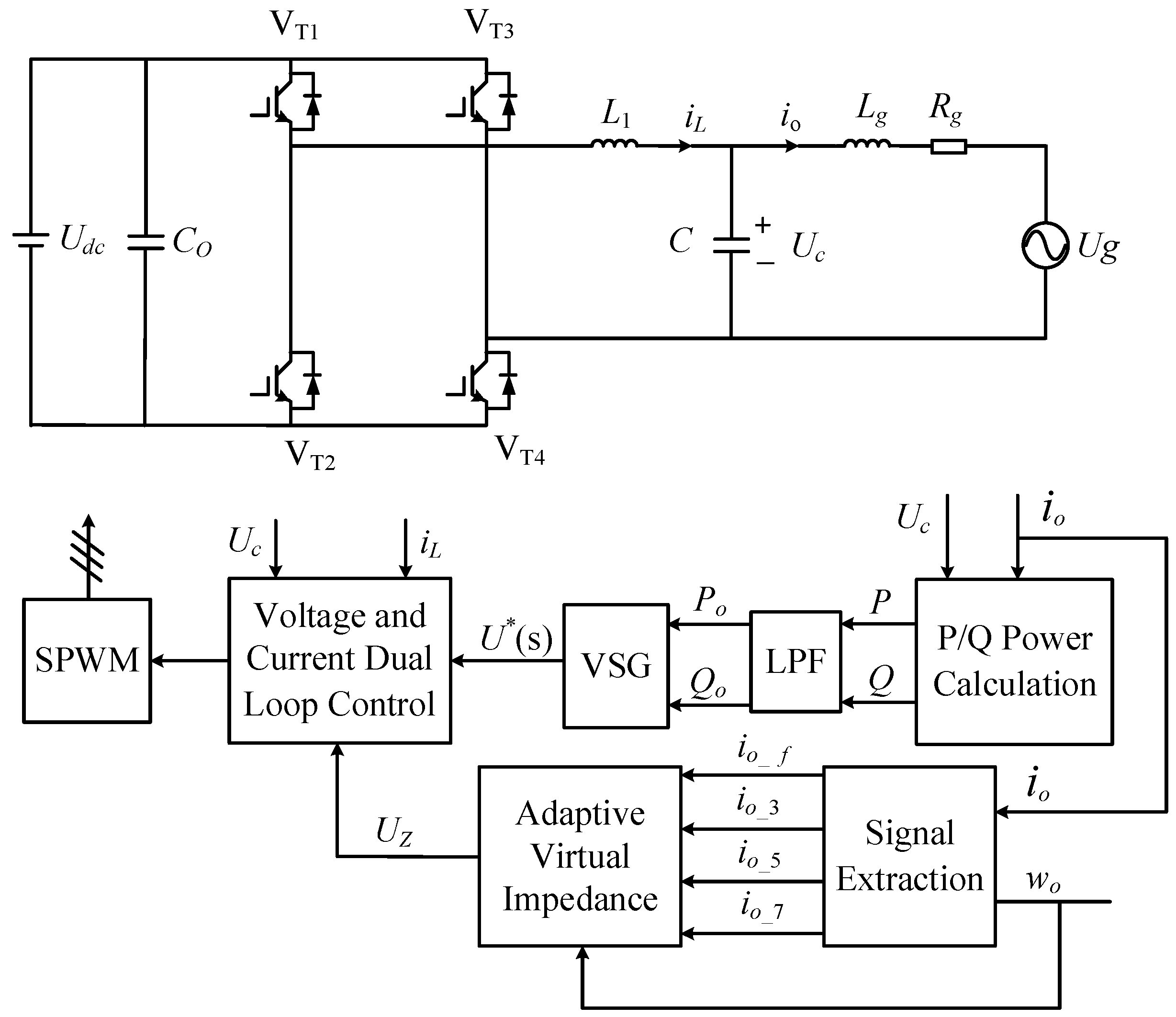
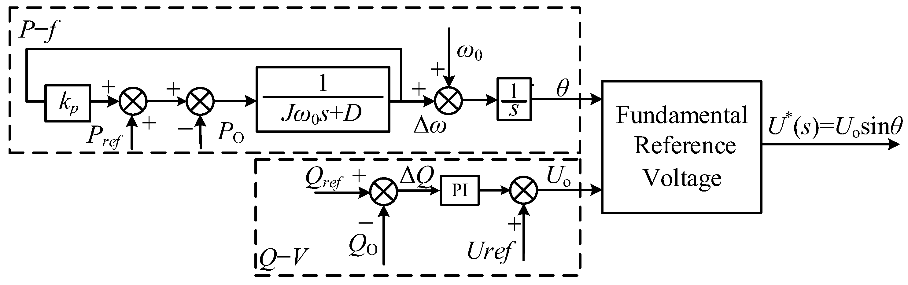
2. Fundamental Principles of the VSG
3. Analysis of the Harmonic Current Mechanism in Grid-Connected Voltage-Source Inverters under Non-Ideal Voltage Conditions
4. Adaptive Virtual Harmonic Resistance and Fundamental Reactance Algorithm
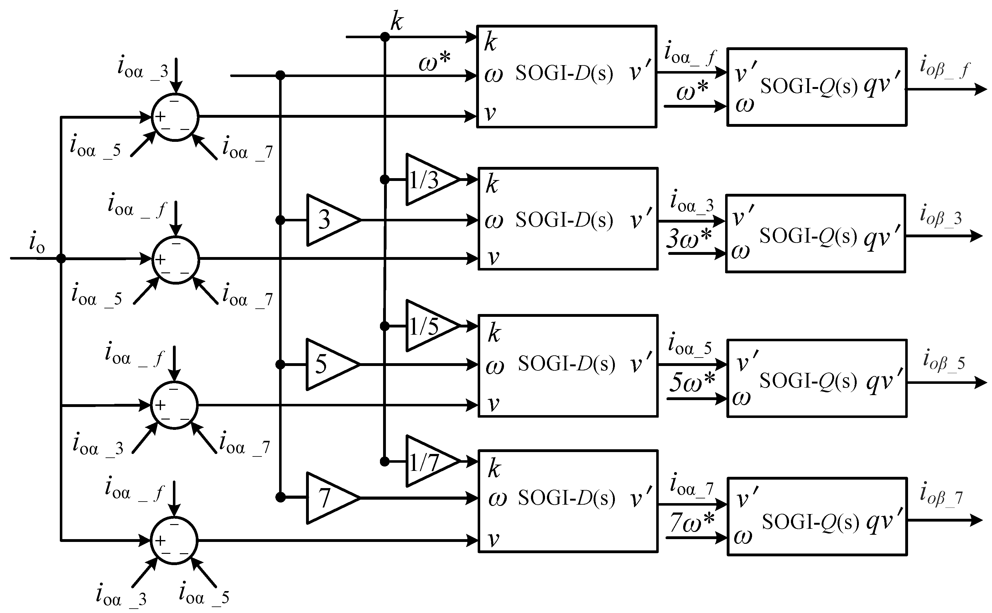
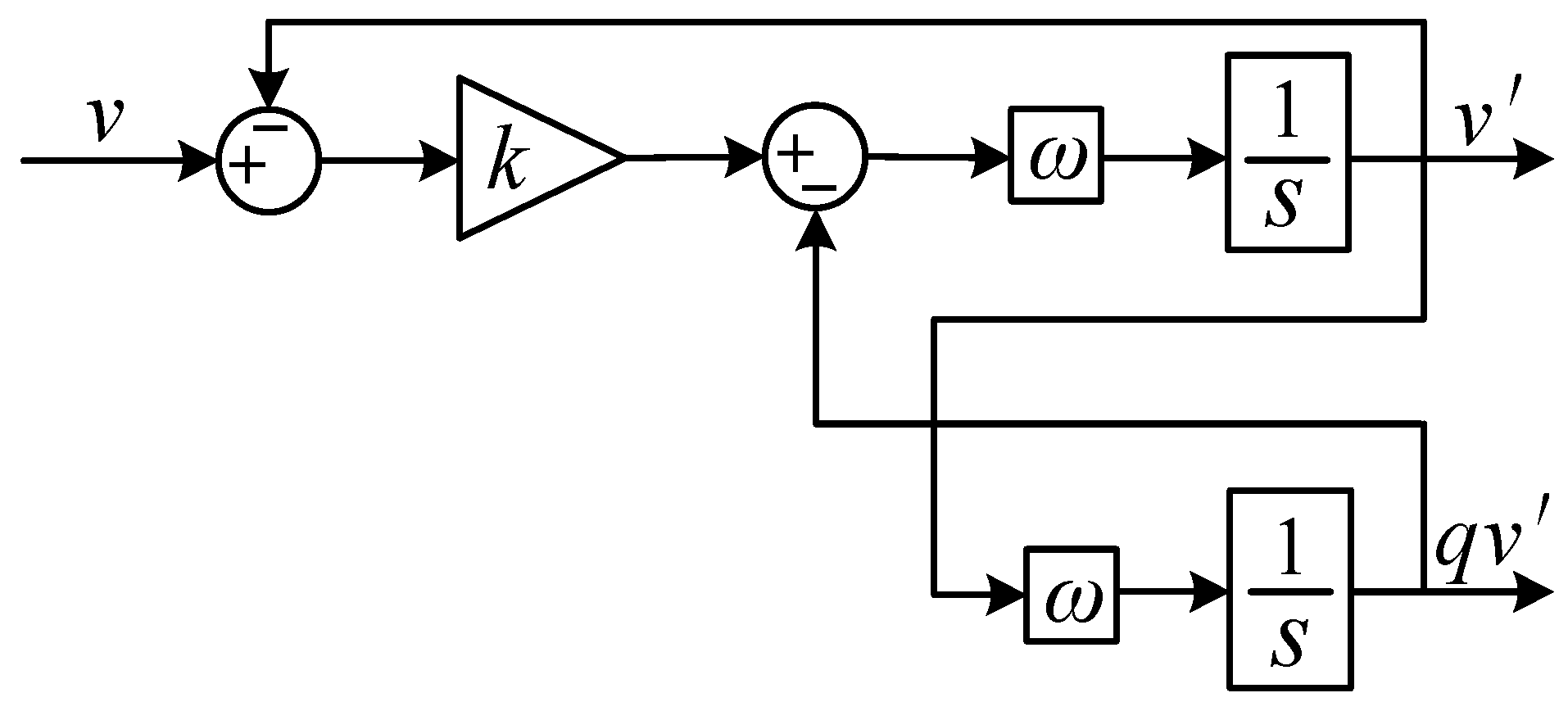
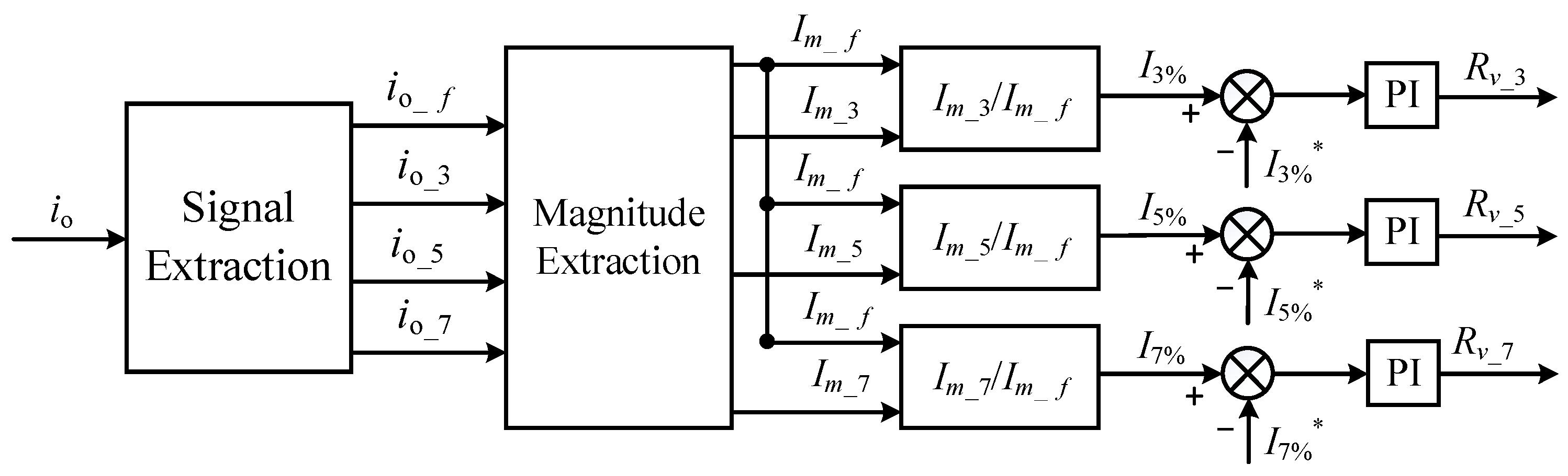
4.1. Adaptive Virtual Harmonic Resistor Implementation Method
4.2. Introduction of the Virtual Harmonic Impedance and Fundamental Reactance into the Equivalent Model
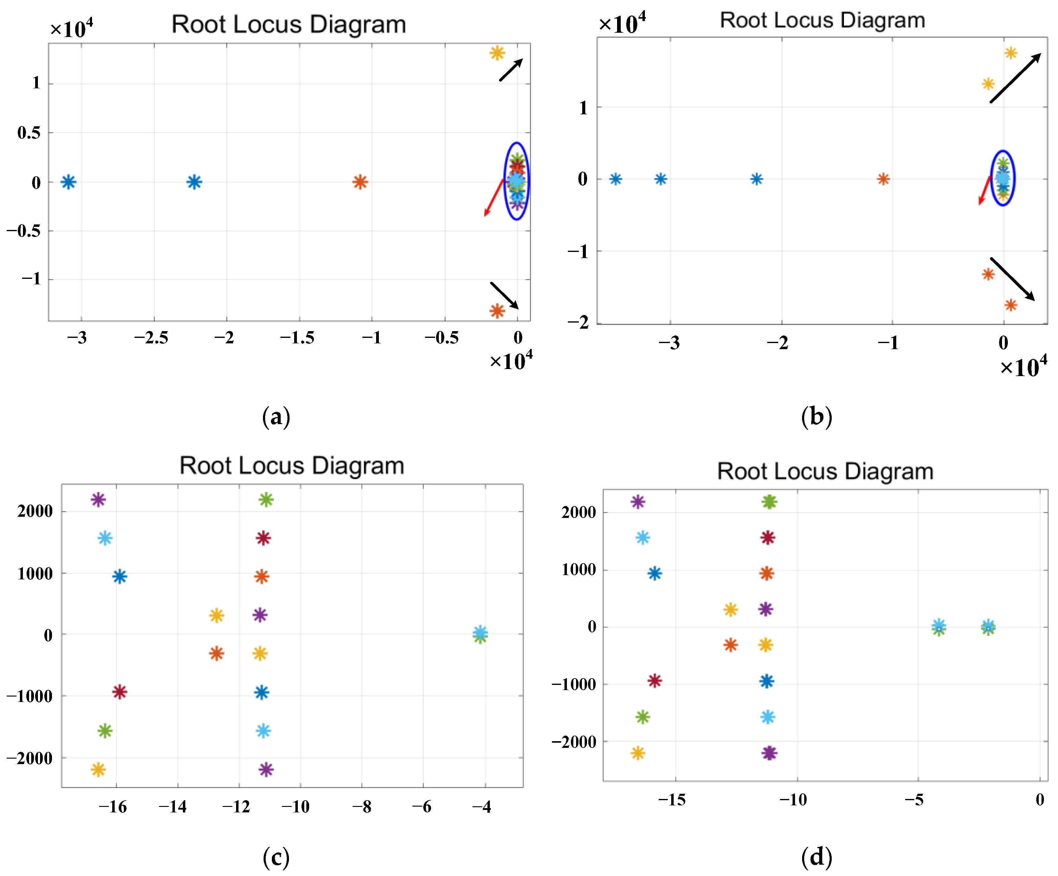
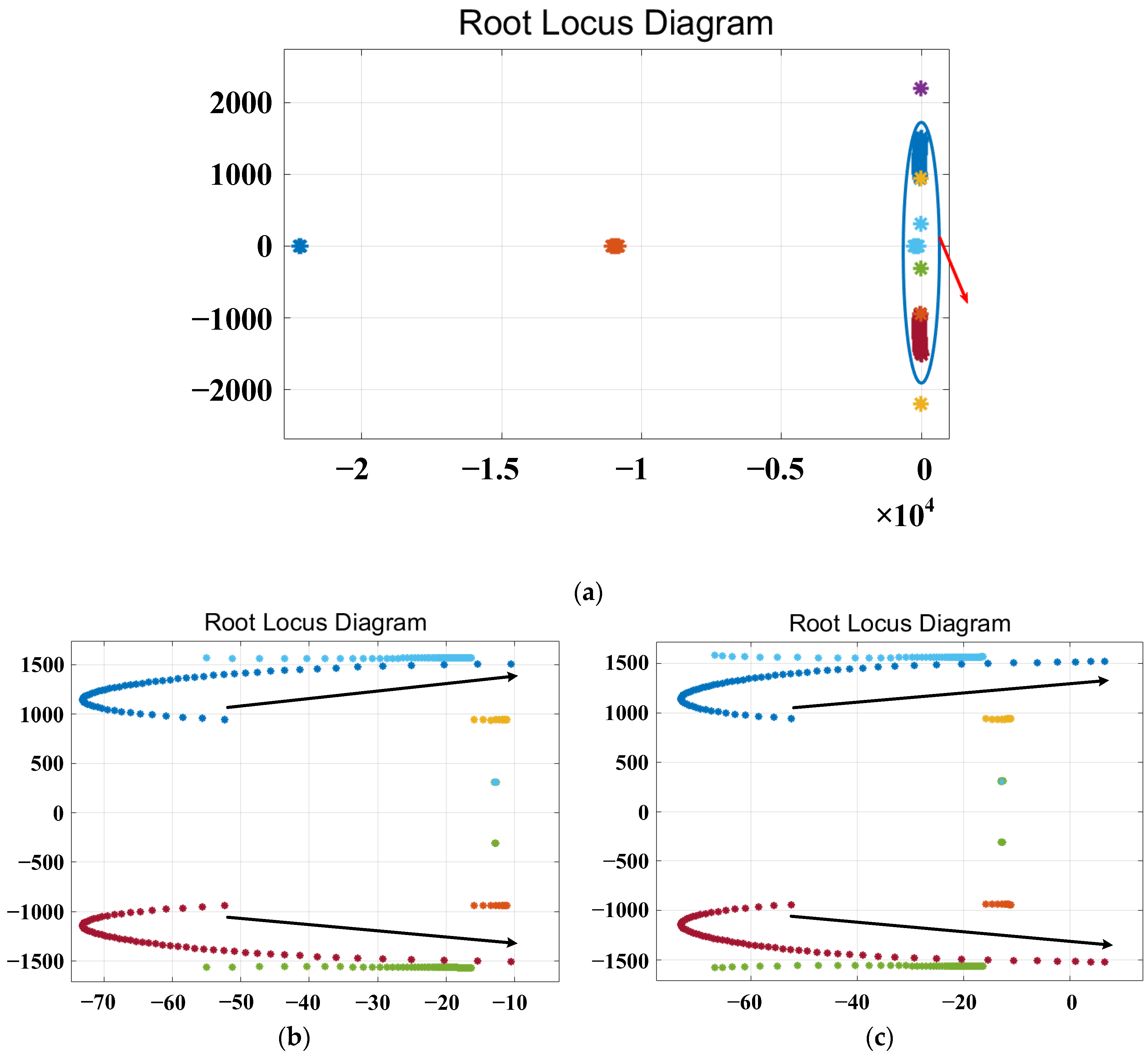
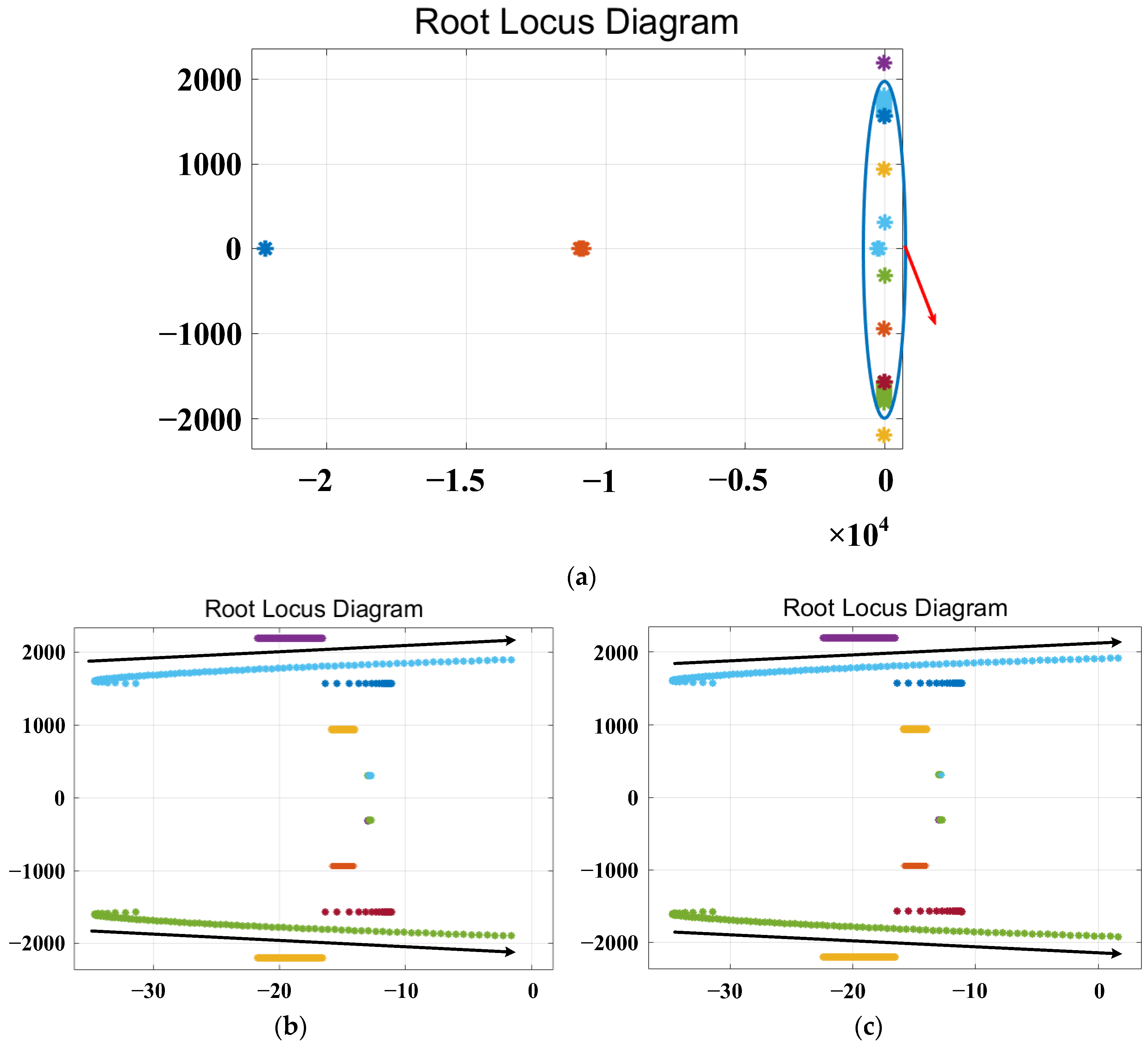
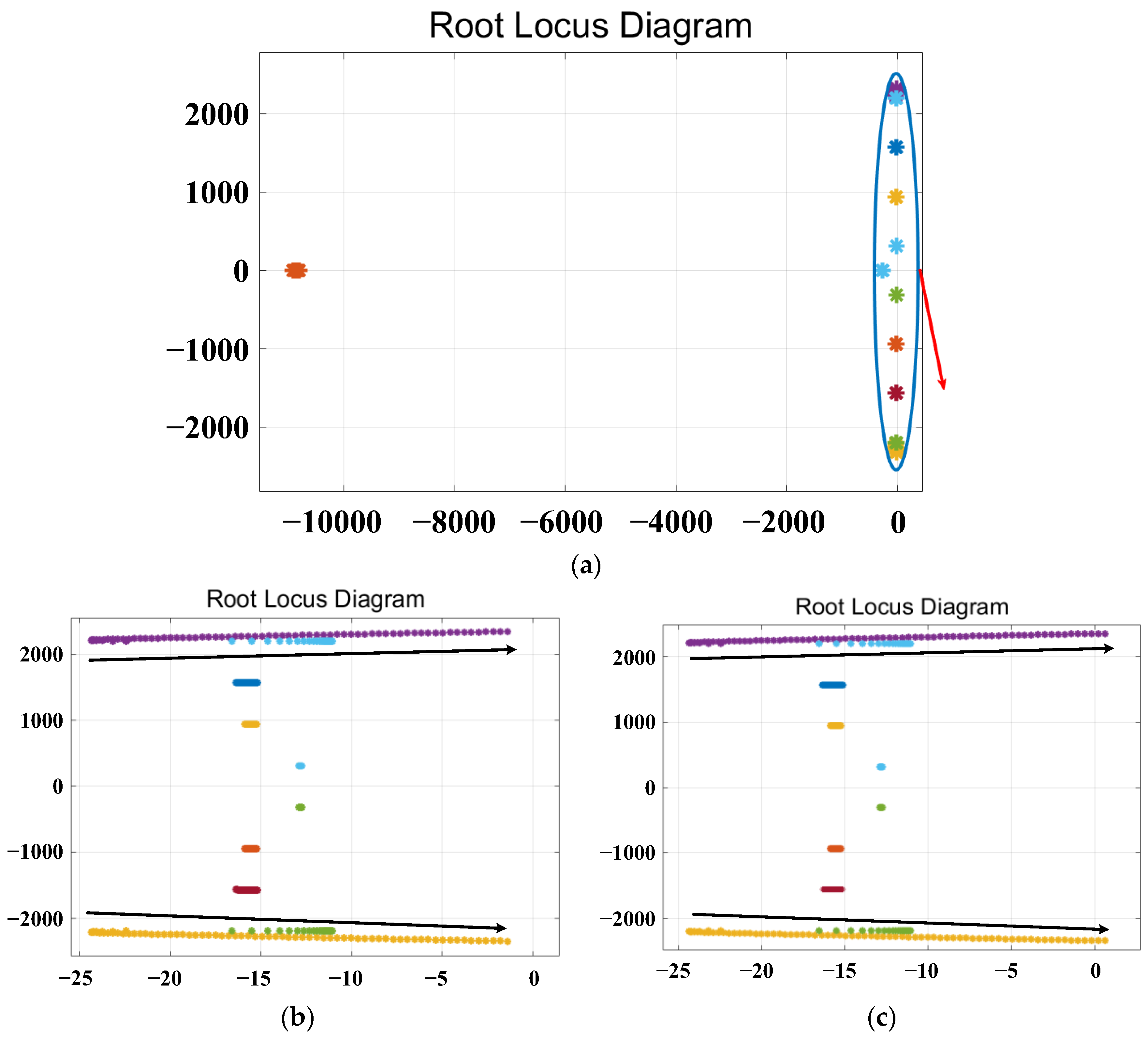
4.3. System Stability Analysis
5. Simulation and Experimental Results
5.1. Simulation Results
5.2. Experimental Results
6. Conclusions
Author Contributions
Funding
Institutional Review Board Statement
Informed Consent Statement
Data Availability Statement
Conflicts of Interest
References
- Wu, Q.H.; Bose, A.; Singh, C.; Chow, J.H.; Mu, G.; Sun, Y.; Liu, Z.; Li, Z.; Liu, Y. Control and Stability of Large-scale Power System with Highly Distributed Renewable Energy Generation: Viewpoints from Six Aspects. CSEE J. Power Energy Syst. 2023, 9, 8–14. [Google Scholar]
- Zhang, H.; Saeedifard, M.; Wang, X.; Meng, Y.; Wang, X. System Harmonic Stability Analysis of Grid-Tied Interlinking Converters Operating Under AC Voltage Control Mode. IEEE Trans. Power Syst. 2022, 37, 4106–4109. [Google Scholar] [CrossRef]
- Borges CL, T.; Martins, V.F. Multistage expansion planning for active distribution networks under demand and distributed generation uncertainties. Electr. Power Energy Syst. 2012, 36, 107–116. [Google Scholar] [CrossRef]
- Razmi, D.; Lu, T.; Papari, B.; Akbari, E.; Fathi, G.; Ghadamyari, M. An Overview on Power Quality Issues and Control Strategies for Distribution Networks with the Presence of Distributed Generation Resources. IEEE Access 2023, 11, 10308–10325. [Google Scholar] [CrossRef]
- Yang, Y.; Xu, J.; Li, C.; Zhang, W.; Wu, Q.; Wen, M.; Blaabjerg, F. A New Virtual Inductance Control Method for Frequency Stabilization of Grid-Forming Virtual Synchronous Generators. IEEE Trans. Ind. Electron. 2023, 70, 441–451. [Google Scholar] [CrossRef]
- Zhang, W.; Sheng, W.; Duan, Q.; Huang, H.; Yan, X. Automatic Generation Control with Virtual Synchronous Renewables. J. Mod. Power Syst. Clean Energy 2023, 11, 267–279. [Google Scholar] [CrossRef]
- Maganti, S.; Padhy, N.P. Analysis and Design of PLL Less Current Control for Weak Grid-Tied LCL-Type Voltage Source Converter. IEEE J. Emerg. Sel. Top. Power Electron. 2022, 10, 4026–4040. [Google Scholar] [CrossRef]
- Chawda, G.S.; Shaik, A.G.; Mahela, O.P.; Padmanaban, S. Performance Improvement of Weak Grid-Connected Wind Energy System Using FLSRF-Controlled DSTATCOM. IEEE Trans. Ind. Electron. 2023, 70, 1565–1575. [Google Scholar] [CrossRef]
- Zhong, P.; Sun, J.; Tian, Z.; Huang, M.; Yu, P.; Zha, X. An Improved Impedance Measurement Method for Grid-Connected Inverter Systems Considering the Background Harmonics and Frequency Deviation. IEEE J. Emerg. Sel. Top. Power Electron. 2021, 9, 4236–4247. [Google Scholar] [CrossRef]
- Lin, Z.; Ruan, X.; Wu, L.; Zhang, H.; Li, W. Multi resonant Component-Based Grid-Voltage-Weighted Feedforward Scheme for Grid-Connected Inverter to Suppress the Injected Grid Current Harmonics under Weak Grid. IEEE Trans. Power Electron. 2020, 35, 9784–9793. [Google Scholar] [CrossRef]
- Zhou, K.; Yang, Y. Multiple harmonics control of single-phase PWM rectifiers. In Proceedings of the 2012 IEEE International Symposium on Industrial Electronics, Hangzhou, China, 28–31 May 2012; pp. 393–396. [Google Scholar]
- Yang, Y.; Yang, Y.; He, L.; Fan, M.; Xiao, Y.; Chen, R.; Xie, M.; Zhang, X.; Zhang, L.; Rodriguez, J. A Novel Cascaded Repetitive Controller of an LC-Filtered H6 Voltage-Source Inverter. IEEE J. Emerg. Sel. Top. Power Electron. 2023, 11, 556–566. [Google Scholar] [CrossRef]
- Ali, M.S.; Wang, L.; Alquhayz, H.; Rehman, O.U.; Chen, G. Performance Improvement of Three-Phase Boost Power Factor Correction Rectifier through Combined Parameters Optimization of Proportional-Integral and Repetitive Controller. IEEE Access 2021, 9, 58893–58909. [Google Scholar] [CrossRef]
- Lyu, M.; Hong, L.; Xu, Q.; Liao, W.; Wu, G.; Huang, S.; Peng, Y.; Long, X. Analysis and Design of PI Plus Repetitive Control for Grid-Side Converters of Direct-Drive Wind Power Systems Considering the Effect of Hardware Sampling Circuits. IEEE Access 2020, 8, 87947–87959. [Google Scholar] [CrossRef]
- Wang, X.; Qin, K.; Ruan, X.; Pan, D.; He, Y.; Liu, F. A Robust Grid-Voltage Feedforward Scheme to Improve Adaptability of Grid-Connected Inverter to Weak Grid Condition. IEEE Trans. Power Electron. 2021, 36, 2384–2395. [Google Scholar] [CrossRef]
- Zheng, Z.; Zhang, L.; Wang, Y.; Lei, Z.; Zou, Y.; Wu, C. Full Grid Voltage Feedforward for Critical Mode LCL-Type Single-Phase Grid-Tied Inverters with Physical Interpretations. IEEE Trans. Power Electron. 2023, 38, 5283–5295. [Google Scholar] [CrossRef]
- Khajeh, K.G.; Farajizadeh, F.; Solatialkaran, D.; Zare, F.; Yaghoobi, J.; Mithulananthan, N. A Full-Feedforward Technique to Mitigate the Grid Distortion Effect on Parallel Grid-Tied Inverters. IEEE Trans. Power Electron. 2022, 37, 8404–8419. [Google Scholar] [CrossRef]
- Ni, R.; Li, Y.W.; Zhang, Y.; Zargari, N.R.; Cheng, Z. Virtual Impedance-Based Selective Harmonic Compensation (VI-SHC) PWM for Current Source Rectifiers. IEEE Trans. Power Electron. 2013, 29, 3346–3356. [Google Scholar] [CrossRef]
- Li, B.; Ding, D.; Wang, Q.; Zhang, G.; Fu, B.; Wang, G.; Xu, D. Input Voltage Feedforward Active Damping-Based Input Current Harmonic Suppression Method for Totem-Pole Bridgeless PFC Converter. IEEE J. Emerg. Sel. Top. Power Electron. 2023, 11, 602–614. [Google Scholar] [CrossRef]
- Khajeh, K.G.; Solatialkaran, D.; Zare, F.; Farajizadeh, F.; Yaghoobi, J.; Nadarajah, M. A Harmonic Mitigation Technique for Multi-Parallel Grid-Connected Inverters in Distribution Networks. IEEE Trans. Power Deliv. 2022, 37, 2843–2856. [Google Scholar] [CrossRef]
- Safamehr, H.; Izadi, I.; Ghaisari, J. Robust Voltage Control for Harmonic Suppression in Islanded Microgrids Using Compensated Disturbance Observer. IEEE Trans. Power Deliv. 2023, 38, 1208–1218. [Google Scholar] [CrossRef]
- Liu, B.; Liu, Z.; Liu, J.; An, R.; Zheng, H.; Shi, Y. An Adaptive Virtual Impedance Control Scheme Based on Small-AC-Signal Injection for Unbalanced and Harmonic Power Sharing in Islanded Microgrids. IEEE Trans. Power Electron. 2019, 34, 12333–12355. [Google Scholar] [CrossRef]
- Ma, K.; Liserre, M.; Blaabjerg, F. Power controllability of three-phase converter with unbalanced AC source. In Proceedings of the 2013 Twenty-Eighth Annual IEEE Applied Power Electronics Conference and Exposition (APEC), Long Beach, CA, USA, 17–21 March 2013; pp. 342–350. [Google Scholar]
- Hasabelrasul, H.; Cai, Z.; Sun, L.; Suo, X.; Matraji, I. Two-Stage Converter Standalone PV-Battery System Based on VSG Control. IEEE Access 2022, 10, 39825–39832. [Google Scholar] [CrossRef]
- Xu, Y.; Nian, H.; Hu, B.; Sun, D. Impedance Modeling and Stability Analysis of VSG Controlled Type-IV Wind Turbine System. IEEE Trans. Energy Convers. 2021, 36, 3438–3448. [Google Scholar] [CrossRef]
- Matas, J.; Martín, H.; de la Hoz, J.; Abusorrah, A.; Al-Turki, Y.; Alshaeikh, H. A New THD Measurement Method with Small Computational Burden Using a SOGI-FLL Grid Monitoring System. IEEE Trans. Power Electron. 2020, 35, 5797–5811. [Google Scholar] [CrossRef]
- Bamigbade, A.; Khadkikar, V.; Zeineldin, H.H.; Moursi, M.S.E.; Hosani, M.A. A Novel Power-Based Orthogonal Signal Generator for Single-Phase Systems. IEEE Trans. Power Deliv. 2021, 36, 469–472. [Google Scholar] [CrossRef]
- Mohamadian, S.; Pairo, H.; Ghasemian, A. A Straightforward Quadrature Signal Generator for Single-Phase SOGI-PLL with Low Susceptibility to Grid Harmonics. IEEE Trans. Ind. Electron. 2022, 69, 6997–7007. [Google Scholar] [CrossRef]
- Wang, X.; Li, Y.W.; Blaabjerg, F.; Loh, P.C. Virtual-Impedance-Based Control for Voltage-Source and Current-Source Converters. IEEE Trans. Power Electron. 2014, 30, 7019–7037. [Google Scholar] [CrossRef]
- Li, S.; Lin, H. A Capacitor-Current-Feedback Positive Active Damping Control Strategy for LCL-Type Grid-Connected Inverter to Achieve High Robustness. IEEE Trans. Power Electron. 2022, 37, 6462–6474. [Google Scholar] [CrossRef]


| Various Control Methods | Adaptive Harmonic Current Suppression | Computational Algorithm Burden | PCC Voltage | Limitation |
|---|---|---|---|---|
| Reference [11] | No | Medium | Do not need | May cause instability of the system |
| References [12,13] | No | High | Do not need | Poor dynamic performance |
| Reference [14] | No | High | Do not need | High complexity of system |
| Reference [15] | No | Media | need | Poor suppression of higher-order harmonics |
| References [16,17] | No | High | need | Amplification of high-frequency signal interference |
| Reference [18] | No | Medium | Do not need | Complexity of high-order harmonic suppression algorithms |
| Reference [19] | No | Media | Do not need | Complex algorithm |
| Reference [20] | No | Medium | need | May cause instability of the system |
| Reference [21] | No | High | Do not need | Complex algorithm |
| Proposed in this paper | Yes | Medium | Do not need | Complexity of high-order harmonic suppression algorithms |
| Parameters | Value | |
|---|---|---|
| Simulation | Experiment | |
| DC voltage Udc | 400 V | 400 V |
| Fundamental voltage amplitude Ug | 314 V | 155.5 V |
| Inverter-side filter inductor L1 | 4 mH | 4 mH |
| Switching frequency fsw | 20 kHz | 20 kHz |
| Grid-side filter inductor and parasitic resistance Lg + Rg | 0.4 Ω + 5 mH | 0.4 Ω + 5 mH |
| Filter capacitor C | 15 uF | 15 uF |
| Virtual fundamental inductor Lv_f | 0.5 mH | 0.5 mH |
| Output power P | - | 1.5 kW |
| Active power reference Pref | 3 kW | - |
| Reactive power reference Qref | 0 var | - |
| 3rd Harmonic Content | 5th Harmonic Content | 7th Harmonic Content | THD of the Grid Current | |
|---|---|---|---|---|
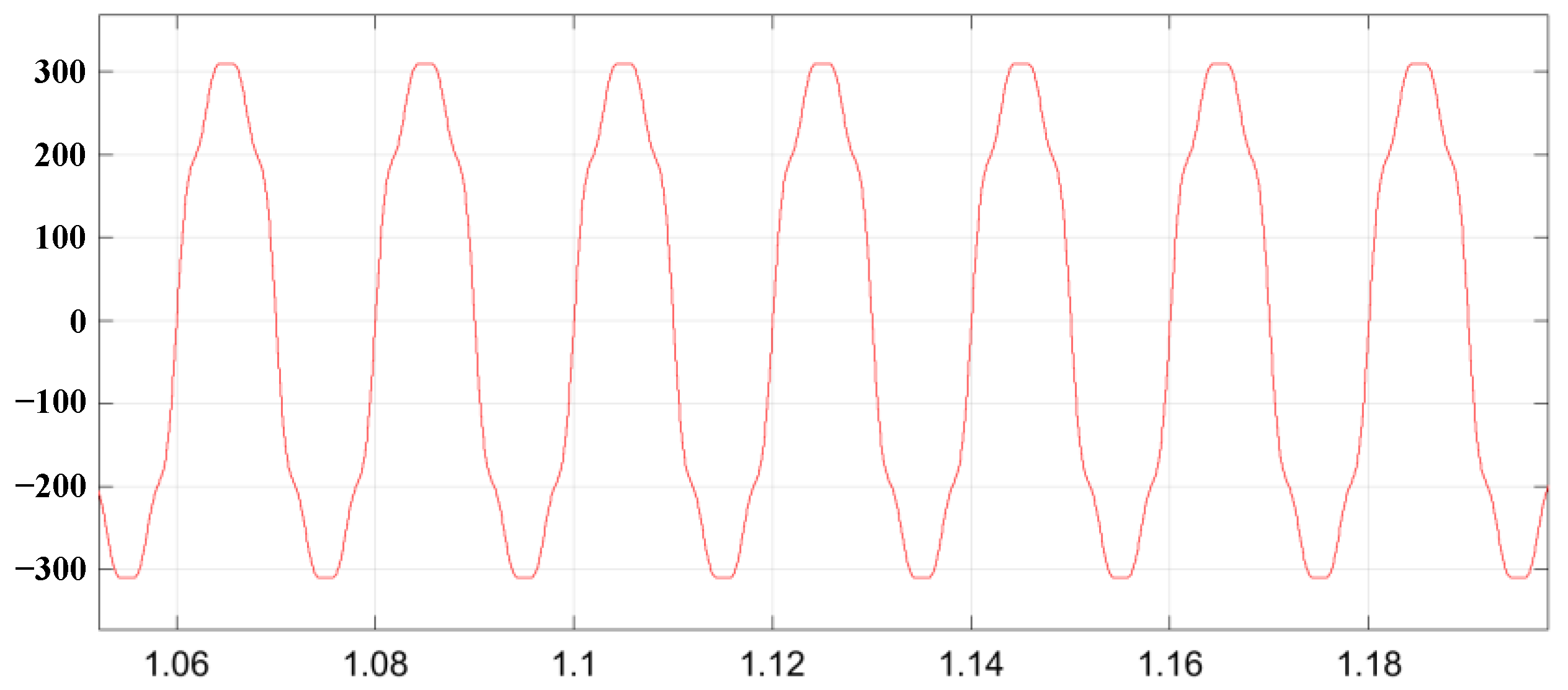
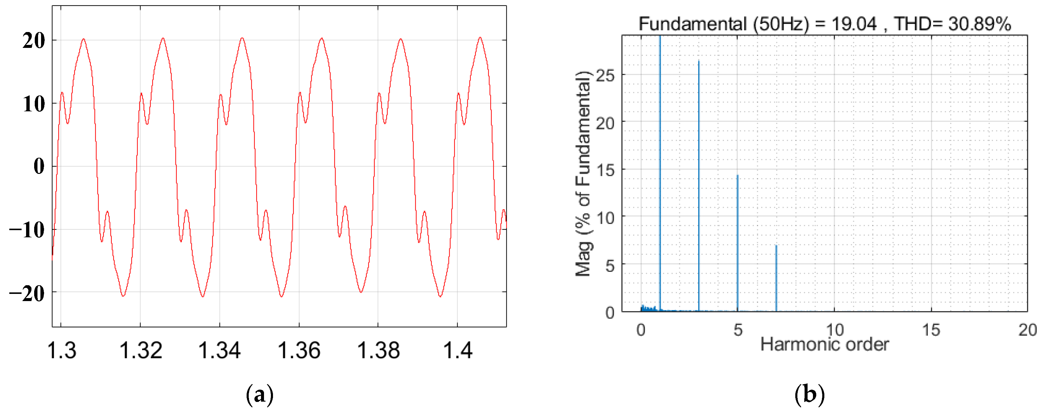
| Without the addition of virtual harmonic impedance | 26.3% | 14.2% | 6.8% | 30.89% |
| Condition 1 | 1.97% | 1.61% | 1.43% | 3.01% |
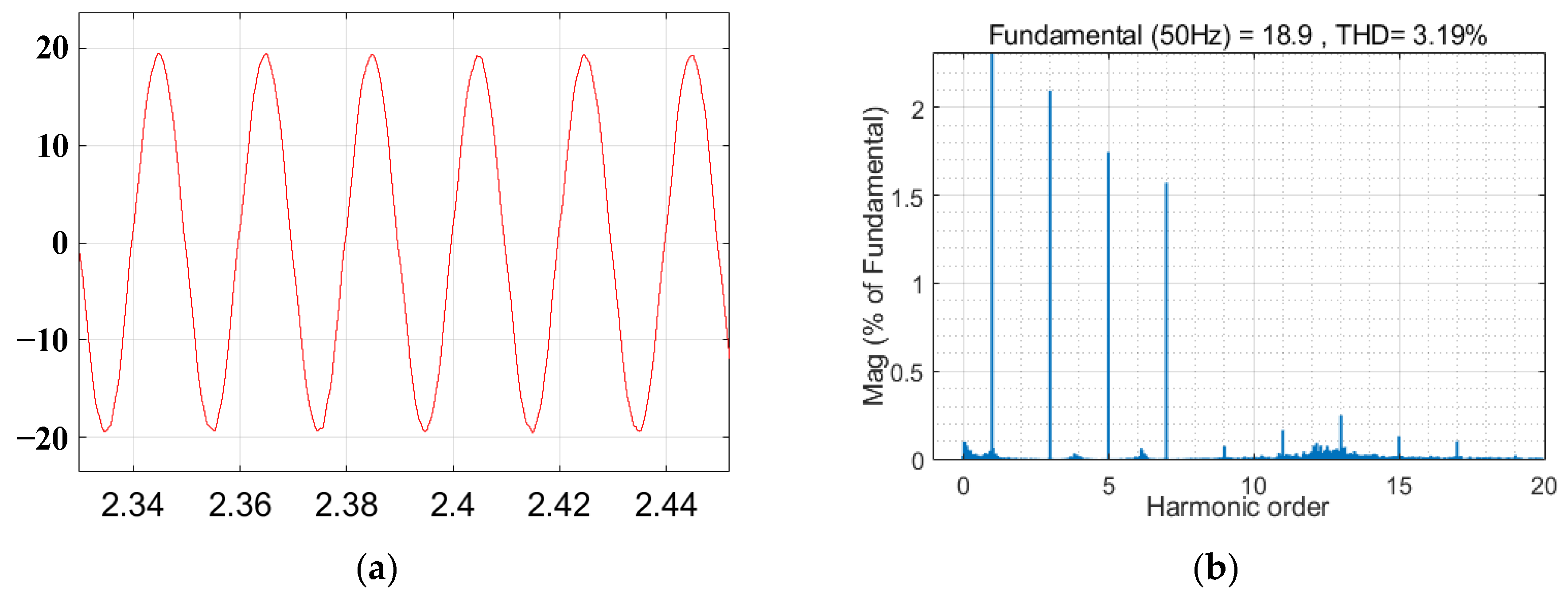
| Condition 2 | 2.08% | 1.74% | 1.54% | 3.19% |
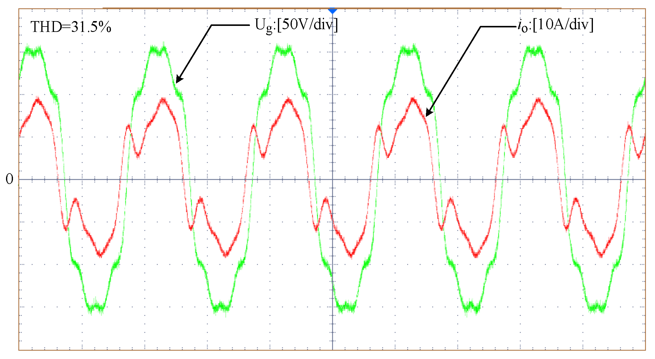
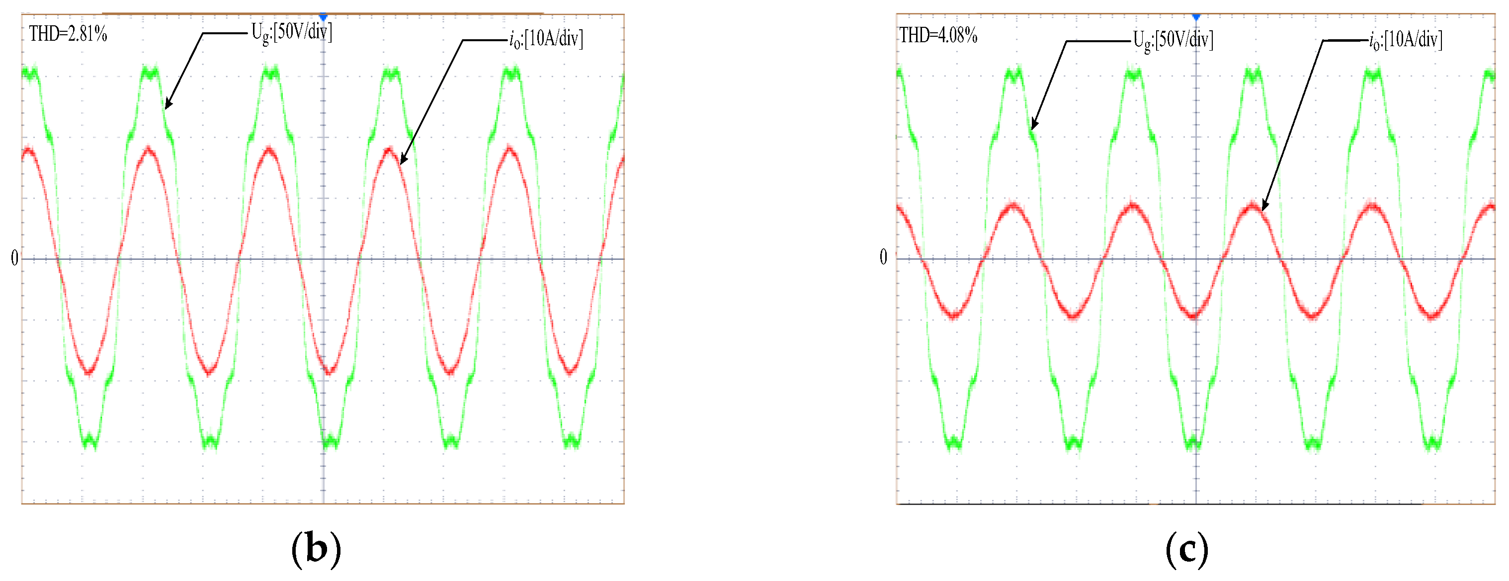
| Different Conditions | THD of the Grid Current |
|---|---|
| Under full-load conditions without the inclusion of the adaptive virtual impedance | 31.5% |
| Under full-load conditions with the inclusion of the adaptive virtual impedance | 2.81% |
| Under half-load conditions with the inclusion of the adaptive virtual impedance | 4.08% |
Disclaimer/Publisher’s Note: The statements, opinions and data contained in all publications are solely those of the individual author(s) and contributor(s) and not of MDPI and/or the editor(s). MDPI and/or the editor(s) disclaim responsibility for any injury to people or property resulting from any ideas, methods, instructions or products referred to in the content. |
© 2023 by the authors. Licensee MDPI, Basel, Switzerland. This article is an open access article distributed under the terms and conditions of the Creative Commons Attribution (CC BY) license (https://creativecommons.org/licenses/by/4.0/).
Share and Cite
Zhong, C.; Zhang, Z.; Zhu, A.; Liang, B. An Adaptive Virtual Impedance Method for Grid-Connected Current Quality Improvement of a Single-Phase Virtual Synchronous Generator under Distorted Grid Voltage. Sensors 2023, 23, 6857. https://doi.org/10.3390/s23156857
Zhong C, Zhang Z, Zhu A, Liang B. An Adaptive Virtual Impedance Method for Grid-Connected Current Quality Improvement of a Single-Phase Virtual Synchronous Generator under Distorted Grid Voltage. Sensors. 2023; 23(15):6857. https://doi.org/10.3390/s23156857
Chicago/Turabian StyleZhong, Caomao, Zhi Zhang, Anan Zhu, and Benxin Liang. 2023. "An Adaptive Virtual Impedance Method for Grid-Connected Current Quality Improvement of a Single-Phase Virtual Synchronous Generator under Distorted Grid Voltage" Sensors 23, no. 15: 6857. https://doi.org/10.3390/s23156857