

CRABR-Net: A Contextual Relational Attention-Based Recognition Network for Remote Sensing Scene Objective


Abstract
:1. Introduction
- (1)
- A complementary relational feature computation module is designed;
- (2)
- An enhanced relational feature calculation module is designed;
- (3)
- A contextual, relational attention-based recognition network is proposed to effectively enhance the performance of RSSOR using CNN.
2. Related Work
2.1. Methods Based on Intuitive Feature
2.2. Methods Based on Statistical Features
2.3. Methods Based on Depth Feature
- CNN without Fusion Method. The method utilizes CNN to acquire local features of the training objectives and then transforms them directly into global features for recognition [35]. According to whether pretraining parameters are used or not, the present method can be categorized into two classes. One class does not use pretraining parameters. Nogueira et al. [36] apply popular CNNs, such as AlexNet, VGG, PatreoNet, etc., to RSSOR, respectively, and achieve good recognition results without pretraining parameters. Another category uses pretraining parameters. Castelluccio et al. [37] demonstrate the importance of adopting pretraining parameters for CNN by importing the pretraining parameters of CaffeNet and GoogLeNet and applying them to RSSOR, respectively;
- CNN with Fusion Method. The methods perform the fusion process on the features of CNN-extracted images. One class of methods utilizes a single CNN to extract features and then fuses them. Yuan et al. [38] directly stitche the last convolutional layer feature and the last fully connected layer feature of VGG-19 as the final representation of the image. Xu et al. [39] processed the convolutional features of layers 4, 7, 10, and 13 of VGG-16 and obtained converged features. The other is utilizing multiple CNNs to draw features, which are then fused. Zhang et al. [40] propose the use of multiple CNNs to extract local features of an image. Liu et al. [41] use CaffeNet and VGG-VD16 to extract deep features and then rearrange and combine them for recognition; Yu et al. [42] use three networks, CaffeNet and its improved network, and improved VGG network, to extract features and fuse them for recognition;
- CNN with AM Method. The methods usually add AM behind the convolutional layer to filter useless information and enhance useful features. For example, the literature [43] added a channel attention mechanism [44] to different stages of DenseNet-121, and Guo et al. [18] added a spatial attention mechanism [45] to the second convolutional module of ResNet-101, and channel attention to the third, fourth, and fifth convolutional modules. Wang et al. [19] propose a mask matrix as a convolutional feature for attention; Fan et al. [46] design an attention mechanism with trunk branches and mask branches for ResNet-50.
3. Methodology
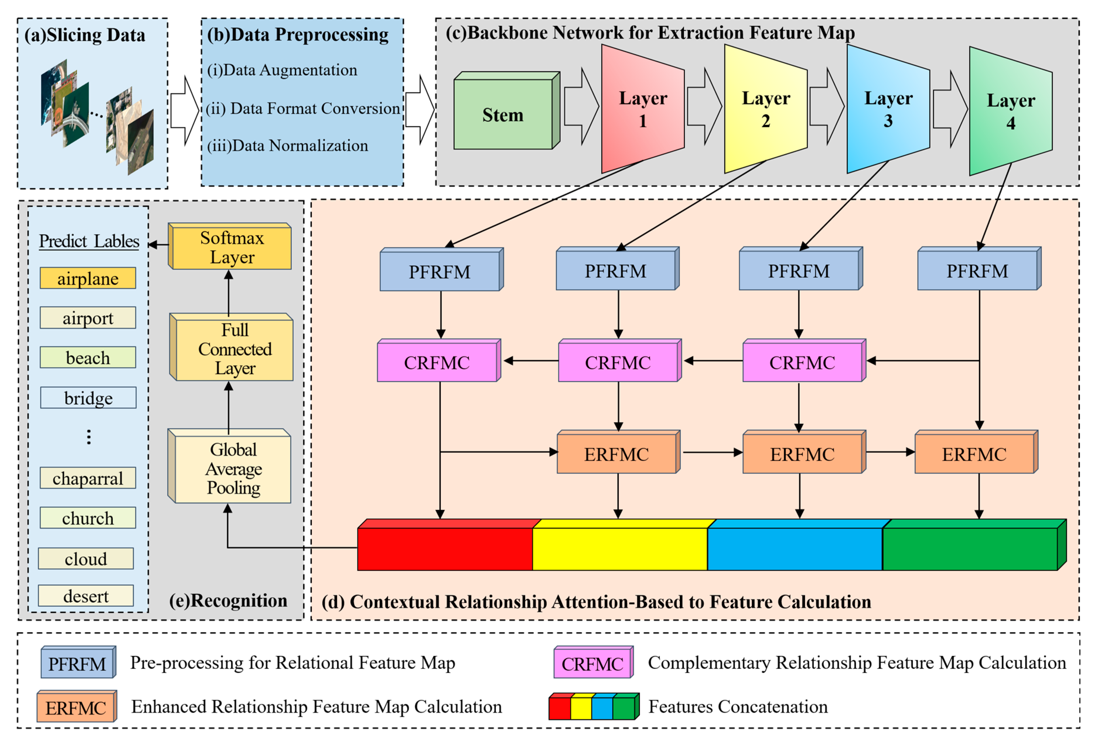
- (a)
- The first step is to divide the data. Divide the remote sensing image dataset into the training dataset and verify the dataset according to a certain ratio (e.g., 4:1);
- (b)
- The second step is data preprocessing. Firstly, augment the remote sensing image data to be input, including randomly cropping to 256 × 256, randomly rotating between −45 degrees and 45 degrees, flipping horizontally with 0.5 probability, and then cropping to 224 × 224; then converting the format, converting the data format to (Batch, Channel, Height, Width); and finally normalizing the data, setting the mean value of Height and Width of every Channel’s Height and Width mean value is set to 0 and standard deviation is set to 1, respectively;
- (c)
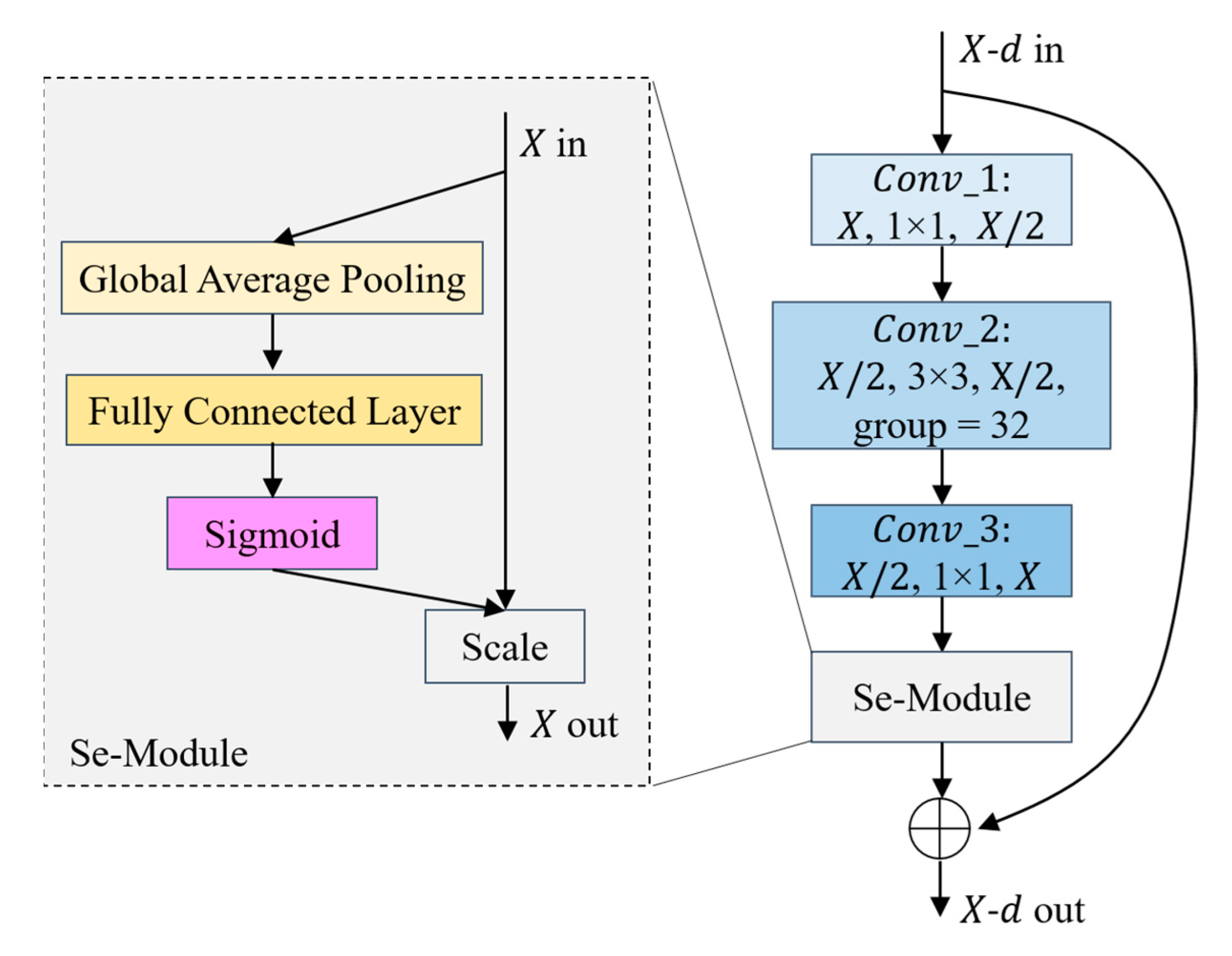
- The third step is to extract features with the backbone network, a Bottleneck is shown in Figure 2. The parameters that have been trained on the Image-Net dataset [47] are imported into the Se-ResNext-50 network, the fully connected layers of the original network are replaced with the network structure designed in steps d and e, and then go on to extract , , , of the four different convolutional layers;
- (d)
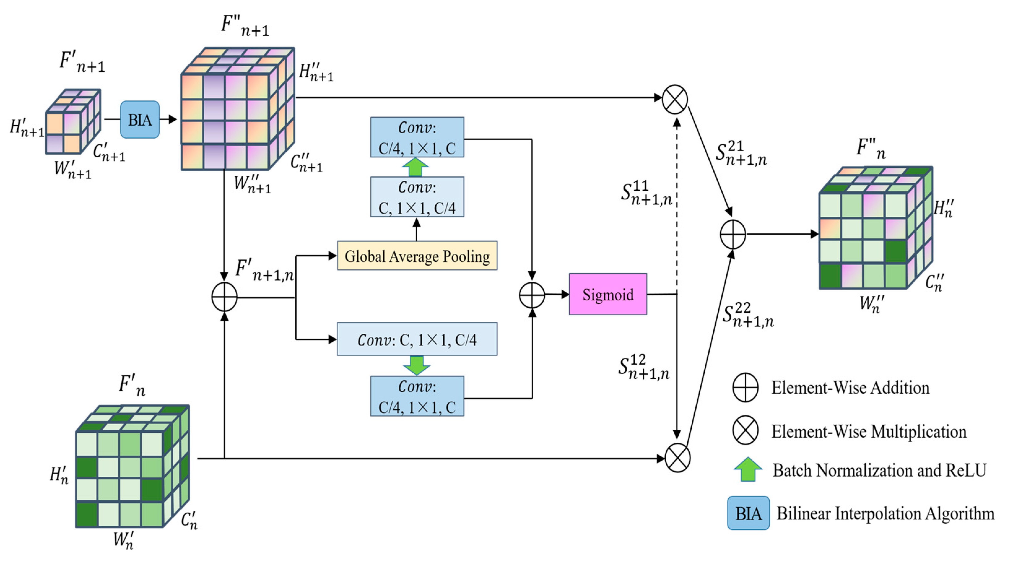
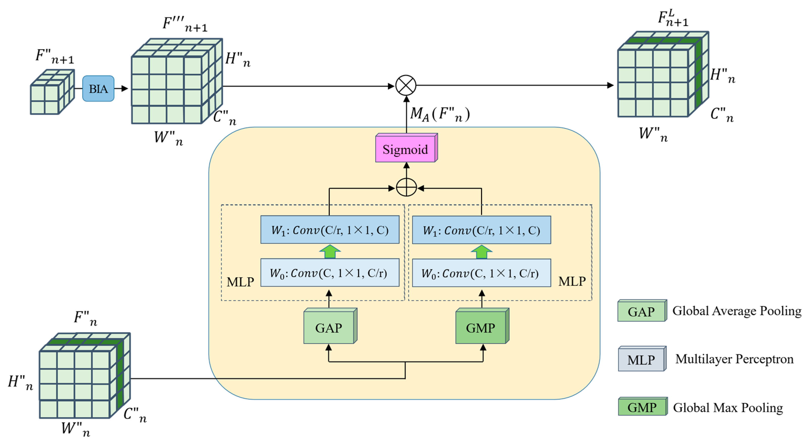
- The fourth step is to compute the relationship enhancement features. (1) PFRFM. Obtain the refined features , , , by using SimAM. (2) CRFMC. Sum the elements at the corresponding positions of and to obtain . Before summing, up-sample by a factor of 2 to obtain . Similarly, we obtain and . For , , , the processing flow shown in Figure 3 can be utilized by using , , respectively. (3) ERFMC. For , is transformed into = [B, 256, 1, 1] and = [B, 256, 1, 1] using GAP and GMP, respectively, and then linearly transformed using MLP to obtain = [B, 256, 1, 1] and = [B, 256, 1, 1], respectively. are obtained through Equation (9). Up-sampling by a factor of 2 yields , and multiplying by yields . Similarly, and can be obtained. Specifically, equals . The process is illustrated in Figure 4. (4) Feature Fusion. Using Equation (11), splice , , , and to obtain = [B, 1024, 56, 56];
- (e)
- The fifth step is to recognize. F is fed into a recognizer consisting of GAP, Fully Connected Layer, and Softmax Layer for scene recognition.
3.1. Backbone Network for Extraction Feature Map
3.2. Preprocessing for Relational Feature Map
3.3. Complementary Relationship Feature Map Calculation
3.4. Enhanced Relationship Feature Map Calculation
3.5. Feature Fusion and Objective Recognition
4. Experiments and Results
4.1. Experiment-Related Settings
4.1.1. Datasets
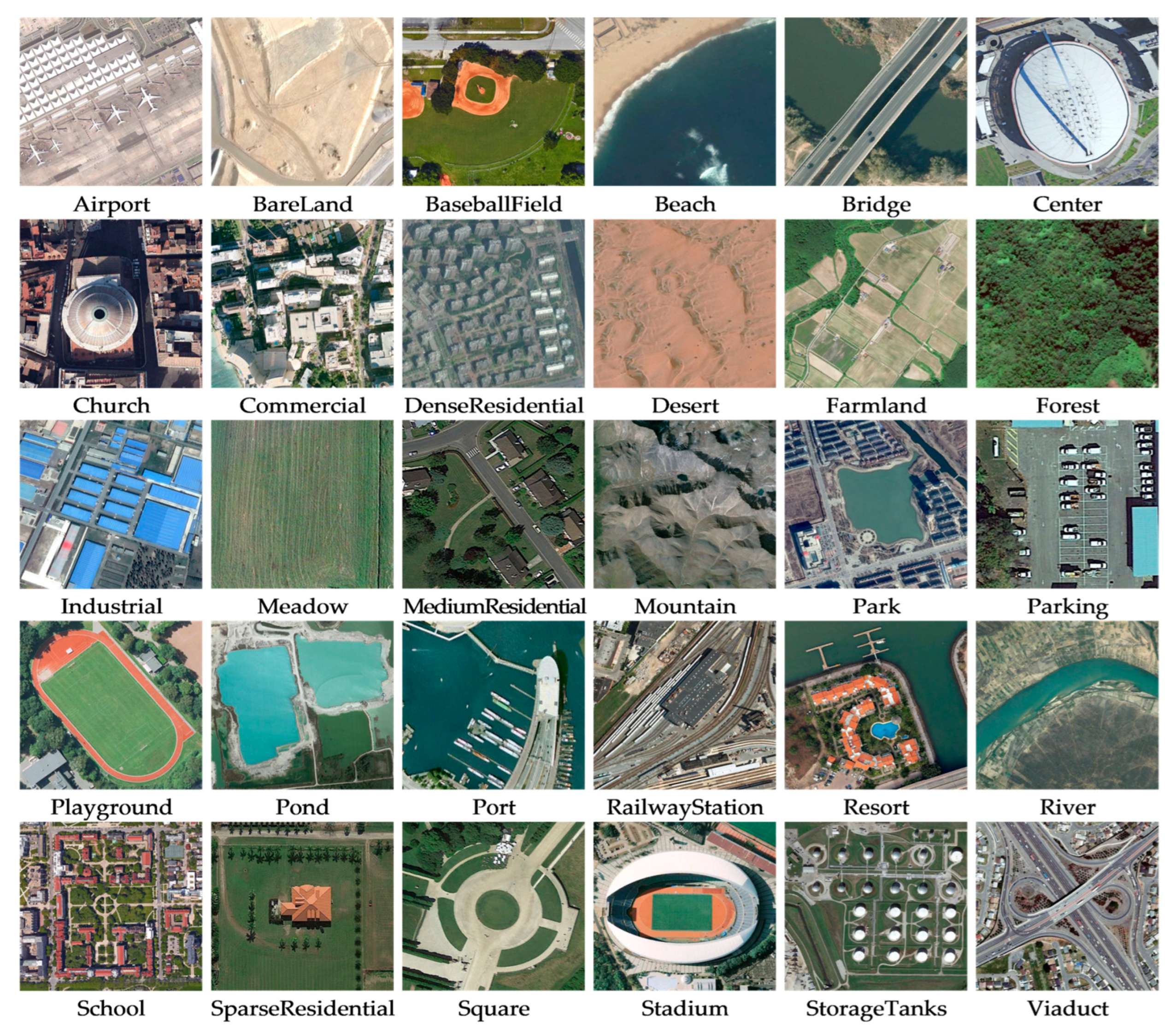
- AID Dataset. It is a massive dataset of airborne scenes, acquired by collecting Google Earth images. It includes 30 categories of feature images of targets such as landforms, terrain, and buildings, and there are approximately 220 to 420 feature images collected for each category. The number of all images together is 10,000; in addition, the pixel size of each image is 600 × 600 [51]. Figure 5 shows instances of the scene objectives for every category within this dataset;
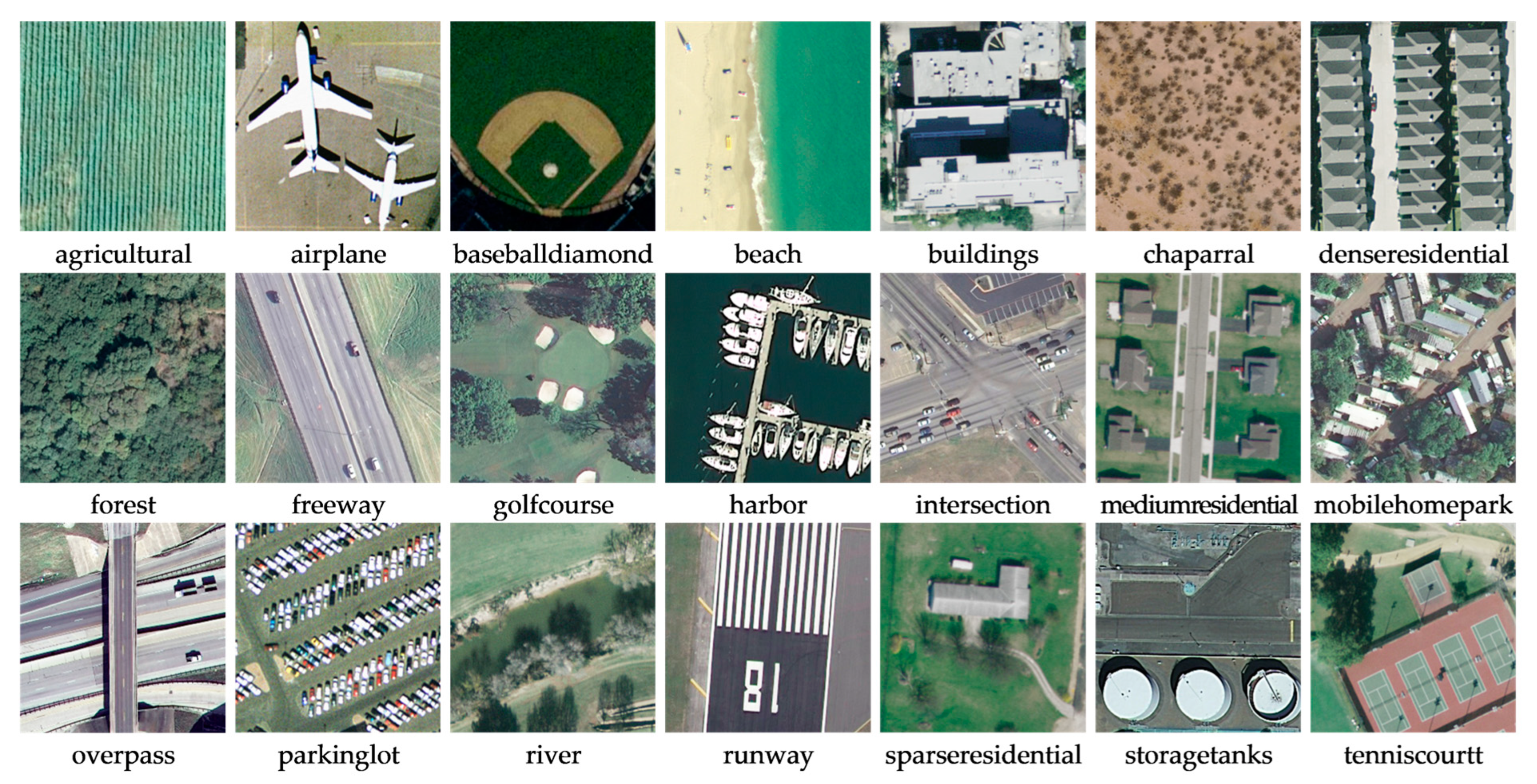
- UC-Merced Dataset. It is an image data representing land use extracted manually by the researchers. These data reflect the land use within the city, and in terms of the main content reflected in the images, there are a total of 21 land use types, with 100 images of each type. The total number of images is 2100, and the size of each type of image is 256 × 256 [52]. Figure 6 shows instances of the scene objectives for every category within this dataset;
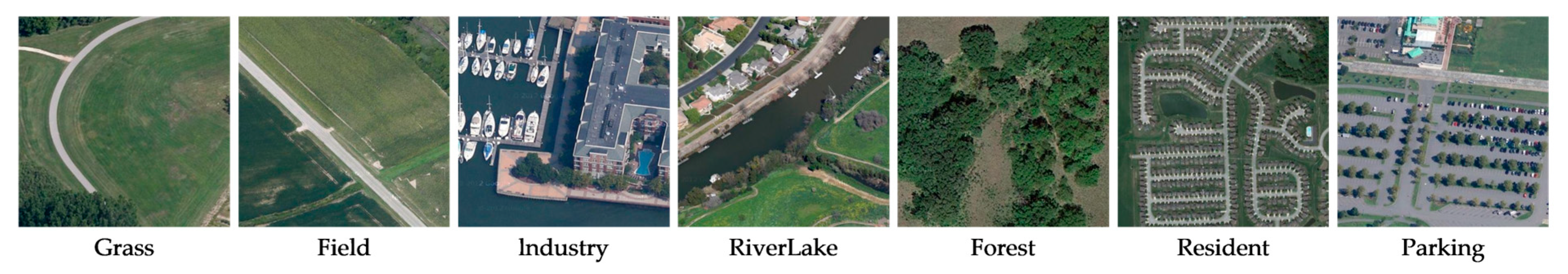
- RSSCN7 Dataset. It is a typical scene target collected from Google Earth, acquired under the conditions of diverse seasonal changes and weather variations, and the data processing is challenging. It contains seven types of features, with a total of 400 images for each type of feature, where each image gets a size of about 400 × 400, for a total of 2800 images [53]. Figure 7 shows instances of the scene objectives for every category within this dataset.
4.1.2. Experimental Environment Setup
4.1.3. Data Preprocessing
4.2. Performance Evaluation Metrics
4.2.1. Accuracy
4.2.2. Confusion Matrix
4.2.3. Precision, Recall, Specificity
4.3. Recognition Results
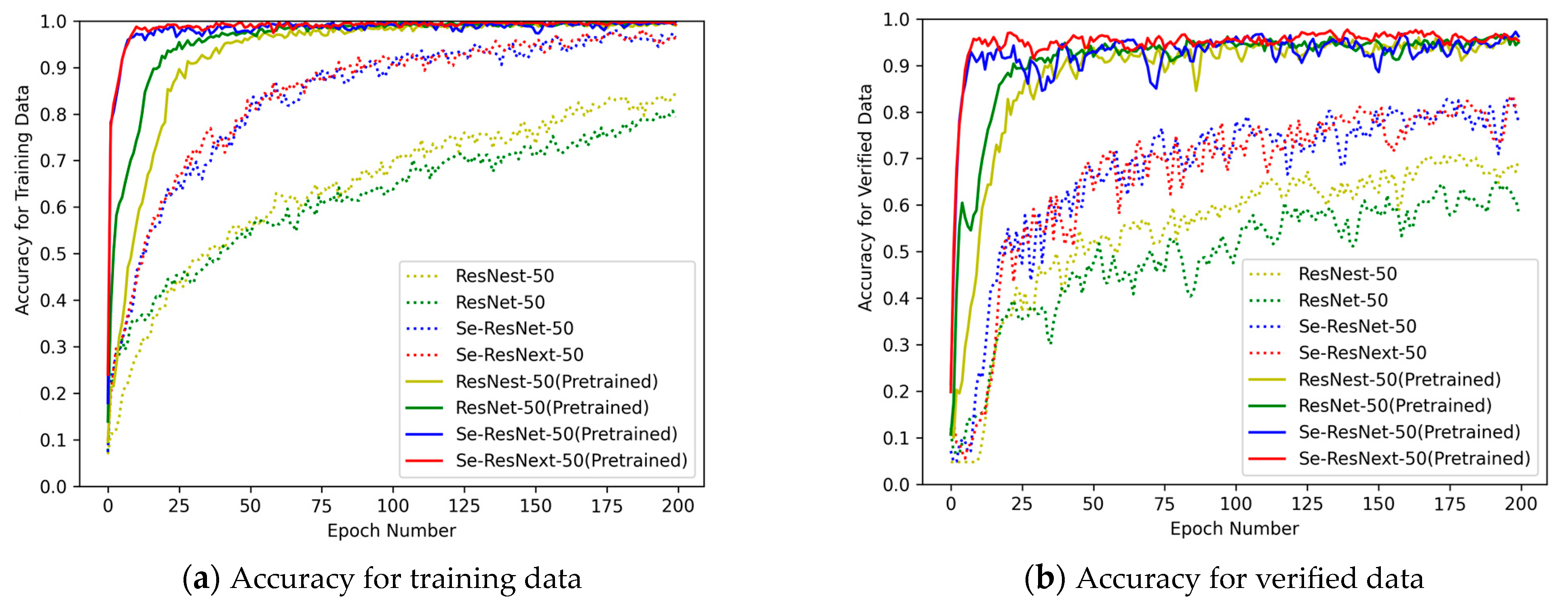
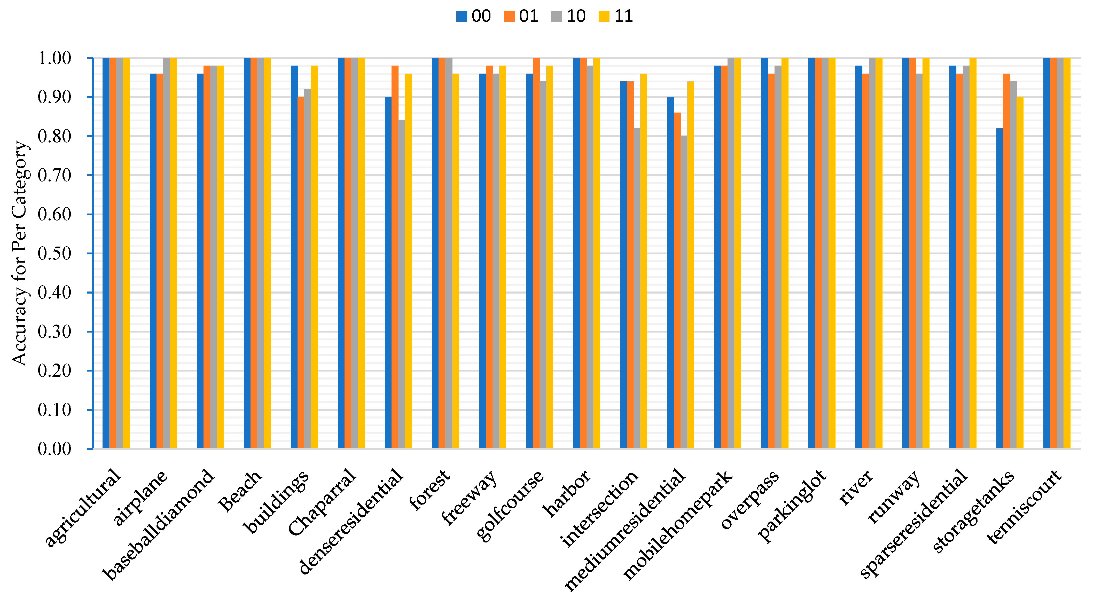
4.3.1. Analysis of Accuracy
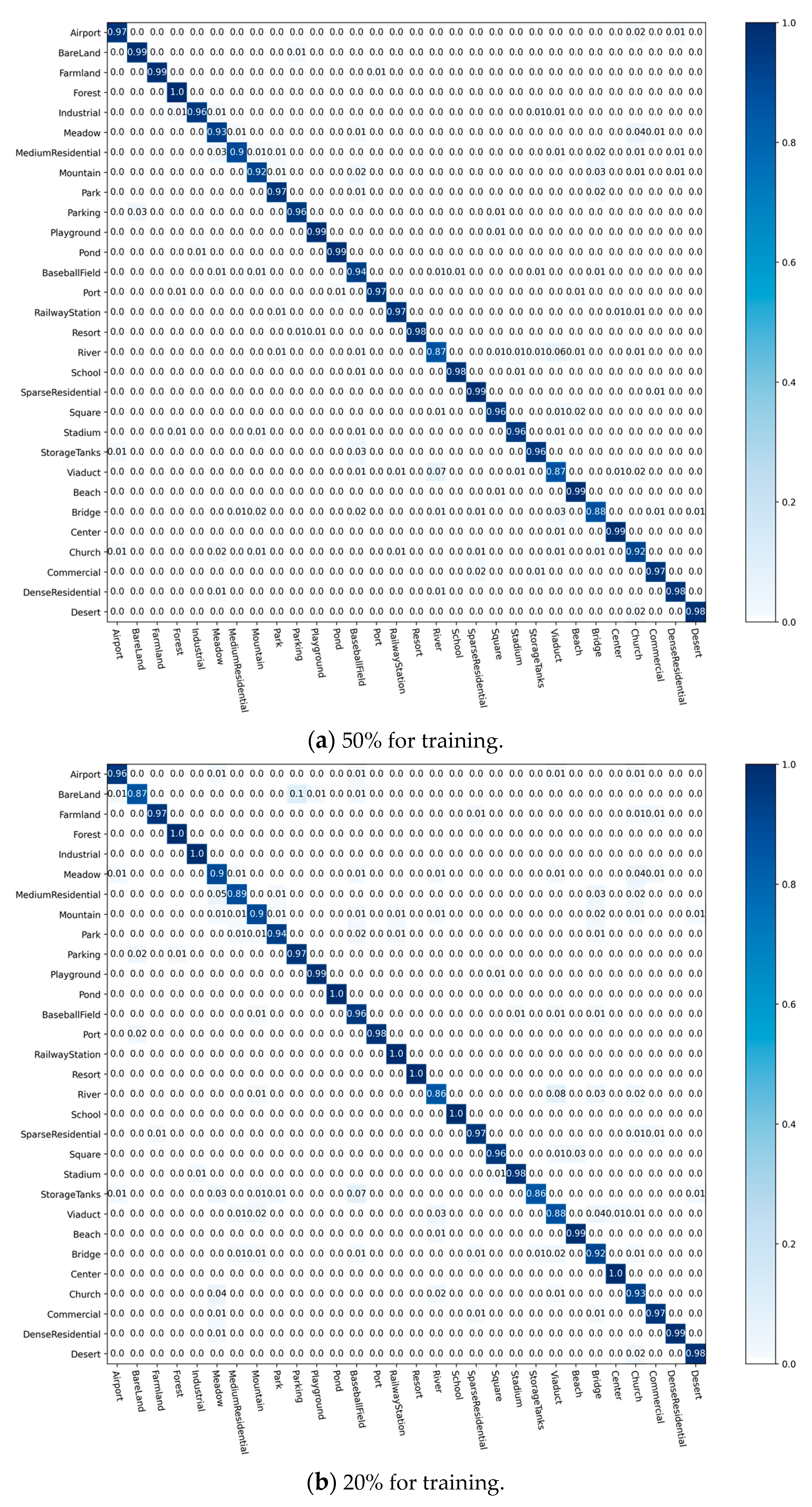
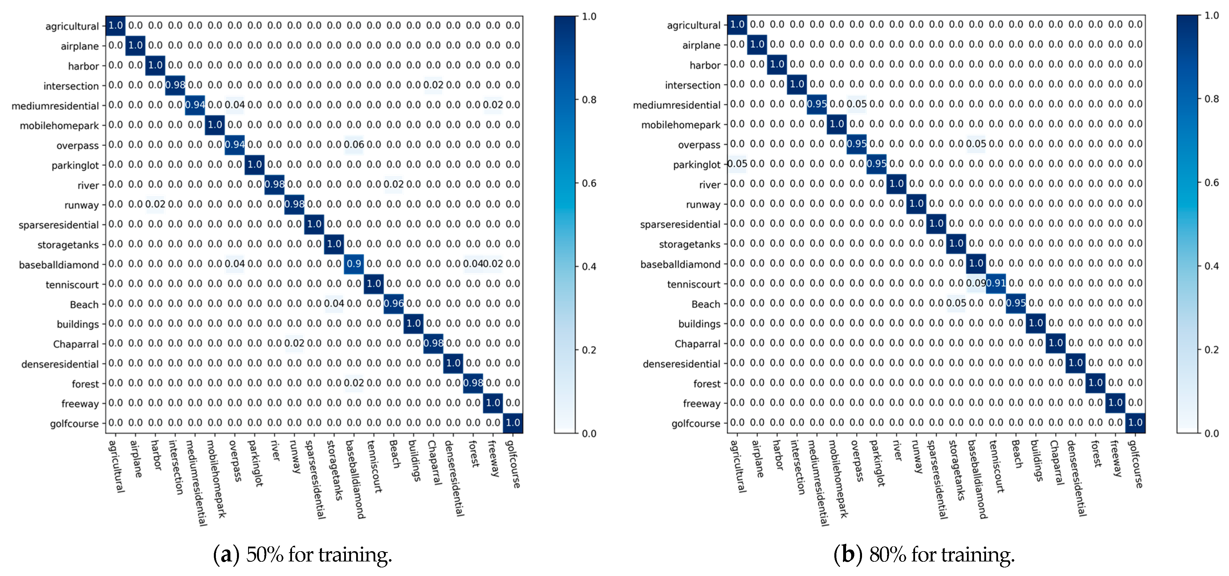
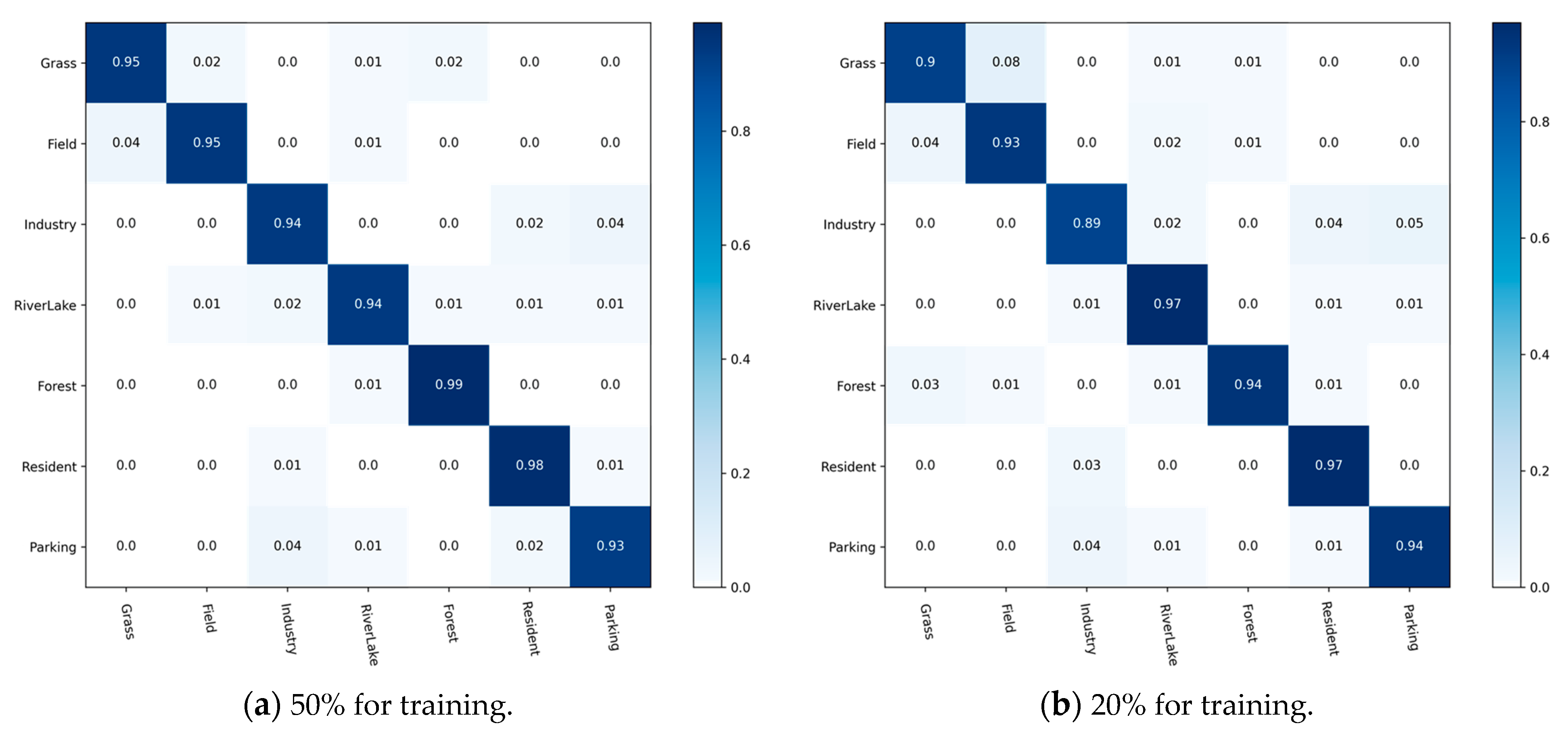
4.3.2. Analysis of Confusion Matrix
5. Discussion
5.1. Effects of Backbone Network
5.2. Effects of Attentional Mechanism
5.3. Effects of MLP, GAP, and GMP
5.4. Effects of Feature Fusion Strategy
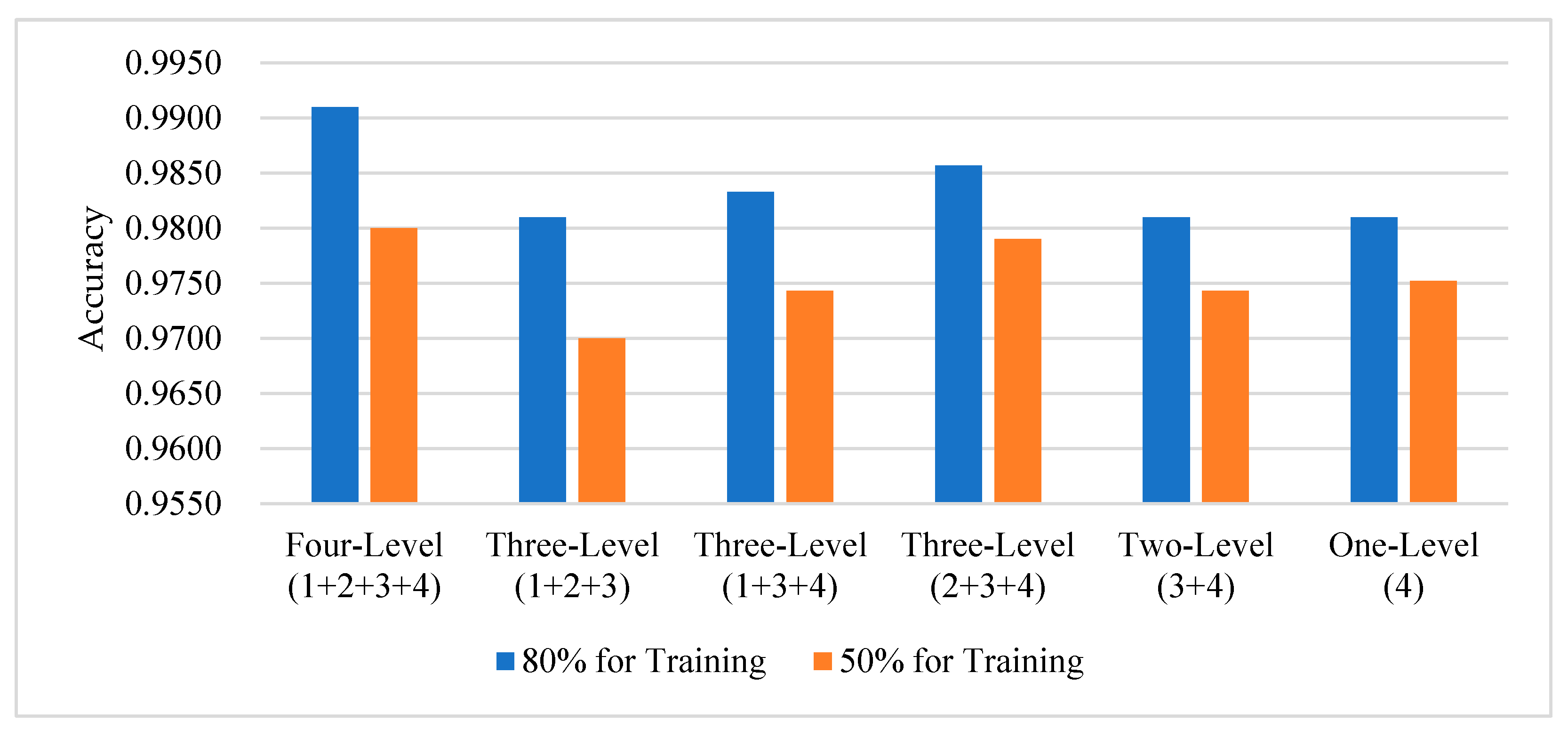
5.5. Effects of Calculation Module
6. Conclusions
Author Contributions
Funding
Institutional Review Board Statement
Informed Consent Statement
Data Availability Statement
Conflicts of Interest
References
- Naushad, R.; Kaur, T.; Ghaderpour, E. Deep transfer learning for land use and land cover classification: A comparative study. Sensors 2021, 21, 8083. [Google Scholar] [CrossRef] [PubMed]
- Liu, Y.; Yao, X.; Gu, Z.; Zhou, Z.; Liu, X.; Chen, X.; Wei, S. Study of the automatic recognition of landslides by using InSAR images and the improved mask R-CNN model in the Eastern Tibet Plateau. Remote Sens. 2022, 14, 3362. [Google Scholar] [CrossRef]
- Wang, Y.; Bashir, S.M.A.; Khan, M.; Ullah, Q.; Wang, R.; Song, Y.; Guo, Z.; Niu, Y. Remote sensing image super-resolution and object detection: Benchmark and state of the art. Expert Syst. Appl. 2022, 197, 116793. [Google Scholar] [CrossRef]
- Peng, F.; Lu, W.; Tan, W.; Qi, K.; Zhang, X.; Zhu, Q. Multi-output network combining GNN and CNN for remote sensing scene classification. Remote Sens. 2022, 14, 1478. [Google Scholar] [CrossRef]
- Han, L.; Zhao, Y.; Lv, H.; Zhang, Y.; Liu, H.; Bi, G. Remote sensing image denoising based on deep and shallow feature fusion and attention mechanism. Remote Sens. 2022, 14, 1243. [Google Scholar] [CrossRef]
- Li, Y.; Wang, J.; Huang, J.; Li, Y. Research on deep learning automatic vehicle recognition algorithm based on RES-YOLO model. Sensors 2022, 22, 3783. [Google Scholar] [CrossRef] [PubMed]
- Song, J.; Gao, S.; Zhu, Y.; Ma, C. A survey of remote sensing image classification based on CNNs. Big Earth Data 2019, 3, 232–254. [Google Scholar] [CrossRef]
- Zhou, Q.; Shen, Z.; Yu, T.; Zhi, P.; Zhao, R. Deep Learning and Visual Perception. In Theories and Practices of Self-Driving Vehicles; Elsevier: Amsterdam, The Netherlands, 2022; pp. 177–216. [Google Scholar] [CrossRef]
- Li, Z.; Liu, F.; Yang, W.; Peng, S.; Zhou, J. A survey of convolutional neural networks: Analysis, applications, and prospects. IEEE Trans. Neural Netw. Learn. Syst. 2021, 33, 6999–7019. [Google Scholar] [CrossRef]
- Zhang, W.; Tang, P.; Zhao, L. Remote sensing image scene classification using CNN-CapsNet. Remote Sens. 2019, 11, 494. [Google Scholar] [CrossRef]
- Hu, S.; Liu, J.; Kang, Z. DeepLabV3+/Efficientnet hybrid network-based scene area judgment for the mars unmanned vehicle system. Sensors 2021, 21, 8136. [Google Scholar] [CrossRef]
- Kim, J.; Chi, M. SAFFNet: Self-attention-based feature fusion network for remote sensing few-shot scene classification. Remote Sens. 2021, 13, 2532. [Google Scholar] [CrossRef]
- Peng, C.; Li, Y.; Jiao, L.; Shang, R. Efficient convolutional neural architecture search for remote sensing image scene classification. IEEE Trans. Geosci. Remote Sens. 2020, 59, 6092–6105. [Google Scholar] [CrossRef]
- He, N.; Fang, L.; Li, S.; Plaza, A.; Plaza, J. Remote sensing scene classification using multilayer stacked covariance pooling. IEEE Trans. Geosci. Remote Sens. 2018, 56, 6899–6910. [Google Scholar] [CrossRef]
- Mei, S.; Yan, K.; Ma, M.; Chen, X.; Zhang, S.; Du, Q. Remote sensing scene classification using sparse representation-based framework with deep feature fusion. IEEE J. Sel. Top. Appl. Earth Obs. Remote Sens. 2021, 14, 5867–5878. [Google Scholar] [CrossRef]
- Shrinivasa, S.; Prabhakar, C. Scene image classification based on visual words concatenation of local and global features. Multimed. Tools Appl. 2022, 81, 1237–1256. [Google Scholar] [CrossRef]
- Vaswani, A.; Shazeer, N.; Parmar, N.; Uszkoreit, J.; Jones, L.; Gomez, A.N.; Kaiser, Ł.; Polosukhin, I. Attention is all you need. In Proceedings of the 31st Conference on Neural Information Processing Systems (NIPS 2017), Long Beach, CA, USA, 4–9 December 2017; Volume 30. [Google Scholar]
- Guo, D.; Xia, Y.; Luo, X. Scene classification of remote sensing images based on saliency dual attention residual network. IEEE Access 2020, 8, 6344–6357. [Google Scholar] [CrossRef]
- Wang, Q.; Liu, S.; Chanussot, J.; Li, X. Scene classification with recurrent attention of VHR remote sensing images. IEEE Trans. Geosci. Remote Sens. 2018, 57, 1155–1167. [Google Scholar] [CrossRef]
- Lin, T.-Y.; Dollár, P.; Girshick, R.; He, K.; Hariharan, B.; Belongie, S. Feature pyramid networks for object detection. In Proceedings of the IEEE Conference on Computer Vision and Pattern Recognition, Honolulu, HI, USA, 21–26 July 2017; pp. 2117–2125. [Google Scholar]
- Murala, S.; Gonde, A.B.; Maheshwari, R.P. Color and texture features for image indexing and retrieval. In Proceedings of the 2009 IEEE International Advance Computing Conference, Patiala, India, 6–7 March 2009; pp. 1411–1416. [Google Scholar]
- Swain, M.J.; Ballard, D.H. Indexing via Color Histograms. In Active Perception and Robot Vision; Springer: Berlin/Heidelberg, Germany, 1992; pp. 261–273. [Google Scholar]
- Tian, Y.; Fang, M.; Kaneko, S.I. Absent Color Indexing: Histogram-Based Identification Using Major and Minor Colors. Mathematics 2022, 10, 2196. [Google Scholar] [CrossRef]
- Haralick, R.M.; Shanmugam, K.; Dinstein, I.H. Textural features for image classification. IEEE Trans. Syst. Man Cybern. 1973, SMC-3, 610–621. [Google Scholar] [CrossRef]
- Partio, M.; Cramariuc, B.; Gabbouj, M.; Visa, A. Rock texture retrieval using gray level co-occurrence matrix. In Proceedings of the 5th Nordic Signal Processing Symposium, Tromsø, Norway, 4–7 October 2002. [Google Scholar]
- Okumura, S.; Maeda, N.; Nakata, K.; Saito, K.; Fukumizu, Y.; Yamauchi, H. Visual categorization method with a Bag of PCA packed Keypoints. In Proceedings of the 2011 4th International Congress on Image and Signal Processing, Shanghai, China, 15–17 October 2011; IEEE: Piscataway, NJ, USA, 2011; pp. 950–953. [Google Scholar]
- Lowe, D.G. Object recognition from local scale-invariant features. In Proceedings of the Seventh IEEE International Conference on Computer Vision, Kerkyra, Greece, 20–27 September 1999; IEEE: Piscataway, NJ, USA, 1999; pp. 1150–1157. [Google Scholar]
- Wang, W.; Poo-Caamaño, G.; Wilde, E.; German, D.M. What is the gist? Understanding the use of public gists on GitHub. In Proceedings of the 2015 IEEE/ACM 12th Working Conference on Mining Software Repositories, Florence, Italy, 16–17 May 2015; IEEE: Piscataway, NJ, USA, 2015; pp. 314–323. [Google Scholar]
- Han, X.; Zhong, Y.; Cao, L.; Zhang, L. Pre-trained alexnet architecture with pyramid pooling and supervision for high spatial resolution remote sensing image scene classification. Remote Sens. 2017, 9, 848. [Google Scholar] [CrossRef]
- Hinton, G.E.; Salakhutdinov, R.R. Reducing the dimensionality of data with neural networks. Science 2006, 313, 504–507. [Google Scholar] [CrossRef] [PubMed]
- Dosovitskiy, A.; Beyer, L.; Kolesnikov, A.; Weissenborn, D.; Zhai, X.; Unterthiner, T.; Dehghani, M.; Minderer, M.; Heigold, G.; Gelly, S. An image is worth 16x16 words: Transformers for image recognition at scale. arXiv 2020, arXiv:2010.11929. [Google Scholar]
- Ketkar, N.; Moolayil, J.; Ketkar, N.; Moolayil, J. Convolutional Neural Networks. In Deep Learning with Python: Learn Best Practices of Deep Learning Models with PyTorch; Springer: Berlin/Heidelberg, Germany, 2021; pp. 197–242. [Google Scholar]
- Li, E.; Du, P.; Samat, A.; Meng, Y.; Che, M. Mid-level feature representation via sparse autoencoder for remotely sensed scene classification. IEEE J. Sel. Top. Appl. Earth Obs. Remote Sens. 2016, 10, 1068–1081. [Google Scholar] [CrossRef]
- Bazi, Y.; Bashmal, L.; Rahhal, M.M.A.; Dayil, R.A.; Ajlan, N.A. Vision transformers for remote sensing image classification. Remote Sens. 2021, 13, 516. [Google Scholar] [CrossRef]
- Penatti, O.A.; Nogueira, K.; Dos Santos, J.A. Do deep features generalize from everyday objects to remote sensing and aerial scenes domains? In Proceedings of the IEEE Conference on Computer Vision and Pattern Recognition Workshops, Boston, MA, USA, 8–10 June 2015; pp. 44–51. [Google Scholar]
- Nogueira, K.; Penatti, O.A.; Dos Santos, J.A. Towards better exploiting convolutional neural networks for remote sensing scene classification. Pattern Recognit. 2017, 61, 539–556. [Google Scholar] [CrossRef]
- Castelluccio, M.; Poggi, G.; Sansone, C.; Verdoliva, L. Land use classification in remote sensing images by convolutional neural networks. arXiv 2015, arXiv:1508.00092. [Google Scholar]
- Yuan, Y.; Fang, J.; Lu, X.; Feng, Y. Remote sensing image scene classification using rearranged local features. IEEE Trans. Geosci. Remote Sens. 2018, 57, 1779–1792. [Google Scholar] [CrossRef]
- Xu, K.; Huang, H.; Li, Y.; Shi, G. Multilayer feature fusion network for scene classification in remote sensing. IEEE Geosci. Remote Sens. Lett. 2020, 17, 1894–1898. [Google Scholar] [CrossRef]
- Zhang, F.; Du, B.; Zhang, L. Scene classification via a gradient boosting random convolutional network framework. IEEE Trans. Geosci. Remote Sens. 2015, 54, 1793–1802. [Google Scholar] [CrossRef]
- Liu, N.; Lu, X.; Wan, L.; Huo, H.; Fang, T. Improving the separability of deep features with discriminative convolution filters for RSI classification. ISPRS Int. J. Geo-Inf. 2018, 7, 95. [Google Scholar] [CrossRef]
- Yu, Y.; Liu, F. Aerial scene classification via multilevel fusion based on deep convolutional neural networks. IEEE Geosci. Remote Sens. Lett. 2018, 15, 287–291. [Google Scholar] [CrossRef]
- Tong, W.; Chen, W.; Han, W.; Li, X.; Wang, L. Channel-attention-based DenseNet network for remote sensing image scene classification. IEEE J. Sel. Top. Appl. Earth Obs. Remote Sens. 2020, 13, 4121–4132. [Google Scholar] [CrossRef]
- Hu, Y.; Wen, G.; Luo, M.; Dai, D.; Ma, J.; Yu, Z. Competitive inner-imaging squeeze and excitation for residual network. arXiv 2018, arXiv:1807.08920. [Google Scholar]
- Bastidas, A.A.; Tang, H. Channel attention networks. In Proceedings of the IEEE/CVF Conference on Computer Vision and Pattern Recognition Workshops, Long Beach, CA, USA, 16–20 June 2019. [Google Scholar]
- Fan, R.; Wang, L.; Feng, R.; Zhu, Y. Attention based residual network for high-resolution remote sensing imagery scene classification. In Proceedings of the IGARSS 2019—2019 IEEE International Geoscience and Remote Sensing Symposium, Yokohama, Japan, 28 July–2 August 2019; IEEE: Piscataway, NJ, USA, 2019; pp. 1346–1349. [Google Scholar]
- Ridnik, T.; Ben-Baruch, E.; Noy, A.; Zelnik-Manor, L. Imagenet-21k pretraining for the masses. arXiv 2021, arXiv:2104.10972. [Google Scholar]
- Hu, J.; Shen, L.; Sun, G. Squeeze-and-excitation networks. In Proceedings of the IEEE Conference on Computer Vision and Pattern Recognition, Salt Lake City, UT, USA, 18–20 June 2018; pp. 7132–7141. [Google Scholar]
- Yang, L.; Zhang, R.-Y.; Li, L.; Xie, X. Simam: A simple, parameter-free attention module for convolutional neural networks. In Proceedings of the International Conference on Machine Learning, Virtual, 18–24 July 2021; PMLR: London, UK, 2021; pp. 11863–11874. [Google Scholar]
- He, J.; Li, L.; Xu, J.; Zheng, C. ReLU deep neural networks and linear finite elements. arXiv 2018, arXiv:1807.03973. [Google Scholar]
- Xia, G.-S.; Hu, J.; Hu, F.; Shi, B.; Bai, X.; Zhong, Y.; Zhang, L.; Lu, X. AID: A benchmark data set for performance evaluation of aerial scene classification. IEEE Trans. Geosci. Remote Sens. 2017, 55, 3965–3981. [Google Scholar] [CrossRef]
- Yang, Y.; Newsam, S. Bag-of-visual-words and spatial extensions for land-use classification. In Proceedings of the 18th SIGSPATIAL International Conference on Advances in Geographic Information Systems, San Jose, CA, USA, 2–5 November 2010; pp. 270–279. [Google Scholar]
- Wu, H.; Liu, B.; Su, W.; Zhang, W.; Sun, J. Hierarchical coding vectors for scene level land-use classification. Remote Sens. 2016, 8, 436. [Google Scholar] [CrossRef]
- Yu, Y.; Liu, F. Dense connectivity based two-stream deep feature fusion framework for aerial scene classification. Remote Sens. 2018, 10, 1158. [Google Scholar] [CrossRef]
- Anwer, R.M.; Khan, F.S.; Van De Weijer, J.; Molinier, M.; Laaksonen, J. Binary patterns encoded convolutional neural networks for texture recognition and remote sensing scene classification. ISPRS J. Photogramm. Remote Sens. 2018, 138, 74–85. [Google Scholar] [CrossRef]
- Sun, H.; Li, S.; Zheng, X.; Lu, X. Remote sensing scene classification by gated bidirectional network. IEEE Trans. Geosci. Remote Sens. 2019, 58, 82–96. [Google Scholar] [CrossRef]
- Cao, R.; Fang, L.; Lu, T.; He, N. Self-attention-based deep feature fusion for remote sensing scene classification. IEEE Geosci. Remote Sens. Lett. 2020, 18, 43–47. [Google Scholar] [CrossRef]
- Hu, F.; Xia, G.-S.; Yang, W.; Zhang, L. Mining deep semantic representations for scene classification of high-resolution remote sensing imagery. IEEE Trans. Big Data 2019, 6, 522–536. [Google Scholar] [CrossRef]
- Zhang, B.; Zhang, Y.; Wang, S. A lightweight and discriminative model for remote sensing scene classification with multidilation pooling module. IEEE J. Sel. Top. Appl. Earth Obs. Remote Sens. 2019, 12, 2636–2653. [Google Scholar] [CrossRef]
- Gao, Y.; Shi, J.; Li, J.; Wang, R. Remote sensing scene classification with dual attention-aware network. In Proceedings of the 2020 IEEE 5th International Conference on Image, Vision and Computing (ICIVC), Beijing, China, 10–12 July 2020; IEEE: Piscataway, NJ, USA, 2020; pp. 171–175. [Google Scholar]
- Shi, C.; Wang, T.; Wang, L. Branch feature fusion convolution network for remote sensing scene classification. IEEE J. Sel. Top. Appl. Earth Obs. Remote Sens. 2020, 13, 5194–5210. [Google Scholar] [CrossRef]
- Liu, B.-D.; Meng, J.; Xie, W.-Y.; Shao, S.; Li, Y.; Wang, Y. Weighted spatial pyramid matching collaborative representation for remote-sensing-image scene classification. Remote Sens. 2019, 11, 518. [Google Scholar] [CrossRef]
- Liu, Y.; Liu, Y.; Ding, L. Scene classification based on two-stage deep feature fusion. IEEE Geosci. Remote Sens. Lett. 2017, 15, 183–186. [Google Scholar] [CrossRef]
- Xu, K.; Huang, H.; Deng, P.; Li, Y. Deep feature aggregation framework driven by graph convolutional network for scene classification in remote sensing. IEEE Trans. Neural Netw. Learn. Syst. 2021, 33, 5751–5765. [Google Scholar] [CrossRef] [PubMed]
- Wang, Q.; Wu, B.; Zhu, P.; Li, P.; Zuo, W.; Hu, Q. ECA-Net: Efficient channel attention for deep convolutional neural networks. In Proceedings of the IEEE/CVF Conference on Computer Vision and Pattern Recognition, Virtual, 13–19 June 2020; pp. 11534–11542. [Google Scholar]
- Woo, S.; Park, J.; Lee, J.-Y.; Kweon, I.S. Cbam: Convolutional block attention module. In Proceedings of the European Conference on Computer Vision (ECCV), Munich, Germany, 8–14 September 2018; pp. 3–19. [Google Scholar]


| Modes | Solutions | Accuracy | |
|---|---|---|---|
| 20% | 50% | ||
| ○ | CaffeNet [49] | 86.86 ± 0.47 | 89.53 ± 0.31 |
| GoogLeNet [49] | 83.44 ± 0.40 | 86.39 ± 0.55 | |
| VGG-VD-16 [49] | 86.59 ± 0.29 | 89.64 ± 0.36 | |
| VGG-16(fine-tuning) [54] | 89.49 ± 0.34 | 93.60 ± 0.64 | |
| ◎ | Two-Steam Fusion [55] | 92.32 ± 0.41 | 94.58 ± 0.25 |
| TEX-Net-LF [56] | 90.87 ± 0.11 | 92.96 ± 0.18 | |
| VGG-16-CapsNet [10] | 91.63 ± 0.19 | 94.74 ± 0.17 | |
| Inception-v3-CapsNet [10] | 93.79 ± 0.13 | 96.32 ± 0.12 | |
| ● | GBNet [54] | 90.16 ± 0.24 | 93.72 ± 0.34 |
| GBNet + global feature [54] | 92.20 ± 0.23 | 95.48 ± 0.12 | |
| AlexNet + SAFF [57] | 87.51 ± 0.36 | 91.83 ± 0.27 | |
| VGG_VD16 + SAFF [57] | 90.28 ± 0.29 | 93.83 ± 0.28 | |
| ARCNet-VGG16 [18] | 88.75 ± 0.40 | 93.10 ± 0.55 | |
| Ours | CRABR-Net | 94.02 ± 0.34 | 96.46 ± 0.23 |
| Modes | Solutions | Accuracy | |
|---|---|---|---|
| 50% | 80% | ||
| ○ | CaffeNet [49] | 93.98 ± 0.67 | 95.02 ± 0.81 |
| GoogLeNet [49] | 92.70 ± 0.60 | 94.31 ± 0.89 | |
| VGG-VD-16 [49] | 94.14 ± 0.69 | 95.21 ± 1.20 | |
| VGG-16(fine-tuning) [54] | 96.57 ± 0.38 | 97.14 ± 0.48 | |
| ◎ | Two-Steam Fusion [55] | 96.97 ± 0.75 | 98.02 ± 1.03 |
| TEX-Net-LF [56] | 95.89 ± 0.37 | 96.62 ± 0.49 | |
| VGG-16-CapsNet [10] | 95.33 ± 0.18 | 98.81 ± 0.22 | |
| MSDS [58] | - | 96.96 ± 0.84 | |
| MLDS [58] | - | 97.88 ± 0.71 | |
| ● | ARCNet-VGG16 [18] | 96.81 ± 0.14 | 99.12 ± 0.40 |
| HONGLIN WU [57] | 95.81 ± 0.98 | 97.43 ± 0.94 | |
| GBNet [54] | 95.71 ± 0.19 | 96.90 ± 0.23 | |
| GBNet+global feature [54] | 97.05 ± 0.19 | 98.57 ± 0.48 | |
| AlexNet + SAFF [57] | 96.13 ± 0.97 | - | |
| VGG_VD16 + SAFF [57] | 97.02 ± 0.78 | - | |
| Ours | CRABR-Net | 98.06 ± 0.24 | 99.20 ± 0.19 |
| Modes | Solutions | Accuracy | |
|---|---|---|---|
| 20% | 50% | ||
| ○ | CaffeNet [49] | 85.57 ± 0.95 | 88.25 ± 0.62 |
| GoogLeNet [49] | 82.55 ± 1.11 | 85.84 ± 0.92 | |
| VGG-VD-16 [49] | 83.98 ± 0.87 | 87.18 ± 0.94 | |
| Fine-turn MobileNet V2 [59] | 89.04 ± 0.17 | 92.46 ± 0.66 | |
| ◎ | TEX-Net-LF [56] | 92.45 ± 0.45 | 94.0 ± 0.55 |
| LCNN-BFF [61] | - | 94.64 ± 0.21 | |
| Yishu Liu [63] | - | 92.37 ± 0.72 | |
| DFAGCN [64] | 94.14 ± 0.44 | ||
| ● | Yue Gao [60] | 91.07 ± 0.65 | 93.25 ± 0.28 |
| Resnet+SPM-CRC [62] | - | 93.86 | |
| Resnet+WSPM-CRC [62] | - | 93.90 | |
| SE-MDPMNet [59] | 92.65 ± 0.13 | 94.71 ± 0.15 | |
| Ours | CRABR-Net | 93.21 ± 0.47 | 95.43 ± 0.79 |
| Class | Precision | Recall | Specificity | |||||||||
|---|---|---|---|---|---|---|---|---|---|---|---|---|
| None | ECA | CBAM | SimAM | None | ECA | CBAM | SimAM | None | ECA | CBAM | SimAM | |
| Agricultural | 1.0 | 1.0 | 1.0 | 0.943 | 1.0 | 1.0 | 1.0 | 1.0 | 1.0 | 1.0 | 1.0 | 0.997 |
| Airplane | 1.0 | 1.0 | 1.0 | 1.0 | 1.0 | 0.96 | 1.0 | 1.0 | 1.0 | 1.0 | 1.0 | 1.0 |
| Baseball diamond | 1.0 | 0.925 | 0.98 | 1.0 | 0.98 | 0.98 | 1.0 | 0.98 | 1.0 | 0.996 | 0.999 | 1.0 |
| Beach | 1.0 | 1.0 | 1.0 | 1.0 | 0.98 | 1.0 | 1.0 | 1.0 | 1.0 | 1.0 | 1.0 | 1.0 |
| Buildings | 0.942 | 0.957 | 0.98 | 0.942 | 0.98 | 0.88 | 0.96 | 0.98 | 0.997 | 0.998 | 0.999 | 0.997 |
| Chaparral | 1.0 | 1.0 | 1.0 | 1.0 | 1.0 | 1.0 | 1.0 | 1.0 | 1.0 | 1.0 | 1.0 | 1.0 |
| Dense residential | 0.906 | 0.907 | 0.906 | 0.923 | 0.96 | 0.98 | 0.96 | 0.96 | 0.995 | 0.995 | 0.995 | 0.996 |
| Forest | 1.0 | 0.962 | 0.98 | 1.0 | 1.0 | 1.0 | 1.0 | 0.96 | 1.0 | 0.998 | 0.999 | 1.0 |
| Freeway | 0.962 | 0.942 | 0.98 | 1.0 | 1.0 | 0.98 | 0.98 | 0.98 | 0.998 | 0.997 | 0.999 | 1.0 |
| Golf course | 0.961 | 0.978 | 1.0 | 0.98 | 0.98 | 0.9 | 0.98 | 0.98 | 0.998 | 0.999 | 1.0 | 0.999 |
| Harbor | 1.0 | 1.0 | 1.0 | 1.0 | 1.0 | 1.0 | 1.0 | 1.0 | 1.0 | 1.0 | 1.0 | 1.0 |
| Intersection | 0.979 | 1.0 | 0.959 | 1.0 | 0.94 | 0.92 | 0.94 | 0.96 | 0.999 | 1.0 | 0.998 | 1.0 |
| Medium residential | 0.938 | 0.939 | 0.939 | 0.959 | 0.9 | 0.92 | 0.92 | 0.94 | 0.997 | 0.997 | 0.997 | 0.998 |
| Mobile home park | 0.98 | 0.98 | 0.98 | 1.0 | 1.0 | 1.0 | 1.0 | 1.0 | 0.999 | 0.999 | 0.999 | 1.0 |
| Overpass | 0.961 | 1.0 | 0.98 | 0.962 | 0.98 | 0.98 | 1.0 | 1.0 | 0.998 | 1.0 | 0.999 | 0.998 |
| Parking lot | 1.0 | 1.0 | 1.0 | 1.0 | 1.0 | 1.0 | 0.98 | 1.0 | 1.0 | 1.0 | 1.0 | 1.0 |
| River | 0.943 | 0.98 | 0.98 | 1.0 | 1.0 | 1.0 | 0.98 | 1.0 | 0.997 | 0.999 | 0.999 | 1.0 |
| Runway | 1.0 | 0.962 | 0.98 | 0.98 | 1.0 | 1.0 | 1.0 | 1.0 | 1.0 | 0.998 | 0.999 | 0.999 |
| Sparse residential | 1.0 | 0.98 | 1.0 | 0.962 | 0.98 | 0.96 | 0.98 | 1.0 | 1.0 | 0.999 | 1.0 | 0.998 |
| Storage tanks | 0.977 | 0.923 | 0.979 | 1.0 | 0.86 | 0.96 | 0.94 | 0.9 | 0.999 | 0.996 | 0.999 | 1.0 |
| Tennis court | 1.0 | 1.0 | 1.0 | 1.0 | 1.0 | 1.0 | 1.0 | 1.0 | 1.0 | 1.0 | 1.0 | 1.0 |
| Maximum rate | 52.38% | 42.86% | 47.62% | 71.43% | 61.90% | 57.14% | 57.14% | 76.19% | 52.38% | 42.86% | 47.62% | 71.43% |
| Scaling Ratio | r = 2 | r = 4 | r = 8 | r = 16 | r = 32 | r = 64 | r = 128 |
|---|---|---|---|---|---|---|---|
| Accuracy | 0.9771 | 0.9762 | 0.9781 | 0.98 | 0.9781 | 0.9752 | 0.9752 |
| GAP | GMP | MLP | Accuracy |
|---|---|---|---|
| × | √ | √ | 0.9771 |
| √ | × | √ | 0.9781 |
| √ | √ | √ | 0.98 |
Disclaimer/Publisher’s Note: The statements, opinions and data contained in all publications are solely those of the individual author(s) and contributor(s) and not of MDPI and/or the editor(s). MDPI and/or the editor(s) disclaim responsibility for any injury to people or property resulting from any ideas, methods, instructions or products referred to in the content. |
© 2023 by the authors. Licensee MDPI, Basel, Switzerland. This article is an open access article distributed under the terms and conditions of the Creative Commons Attribution (CC BY) license (https://creativecommons.org/licenses/by/4.0/).
Share and Cite
Guo, N.; Jiang, M.; Gao, L.; Tang, Y.; Han, J.; Chen, X. CRABR-Net: A Contextual Relational Attention-Based Recognition Network for Remote Sensing Scene Objective. Sensors 2023, 23, 7514. https://doi.org/10.3390/s23177514
Guo N, Jiang M, Gao L, Tang Y, Han J, Chen X. CRABR-Net: A Contextual Relational Attention-Based Recognition Network for Remote Sensing Scene Objective. Sensors. 2023; 23(17):7514. https://doi.org/10.3390/s23177514
Chicago/Turabian StyleGuo, Ningbo, Mingyong Jiang, Lijing Gao, Yizhuo Tang, Jinwei Han, and Xiangning Chen. 2023. "CRABR-Net: A Contextual Relational Attention-Based Recognition Network for Remote Sensing Scene Objective" Sensors 23, no. 17: 7514. https://doi.org/10.3390/s23177514
APA StyleGuo, N., Jiang, M., Gao, L., Tang, Y., Han, J., & Chen, X. (2023). CRABR-Net: A Contextual Relational Attention-Based Recognition Network for Remote Sensing Scene Objective. Sensors, 23(17), 7514. https://doi.org/10.3390/s23177514