
Research on Path Planning and Path Tracking Control of Autonomous Vehicles Based on Improved APF and SMC

Abstract
:1. Introduction
- 1.
- This study presents a method for setting the action area of a repulsive force field by analyzing the change in obstacle velocity. The detection process is divided into two areas. First, within a 120° range in front of the vehicle, a forward detection radius function is formulated based on the relative velocity between the closest obstacle and the vehicle. This function determines the detection area for obstacles in front. Similarly, a rear detection radius function is developed to cover a 240° range behind the vehicle for rear detection purposes. By considering only obstacles within the detection range, it saves computational time by ignoring irrelevant obstacle repulsion fields. This approach ensures both the accuracy and real-time performance of the path planning process.
- 2.
- In response to the problem of unreachable targets and local optima in traditional APF methods, this study introduces the concept of virtual sub-target points and a target point distance factor. These sub-target points are randomly generated within a certain radius around the target point to replace the original target point when the resultant force becomes zero during obstacle movement. By doing so, the resultant force is always maintained as non-zero, preventing the vehicle from becoming stuck in local minima. Additionally, the distance factor for the target point is included in the formula to ensure that the total force becomes zero when the vehicle reaches the target point.
- 3.
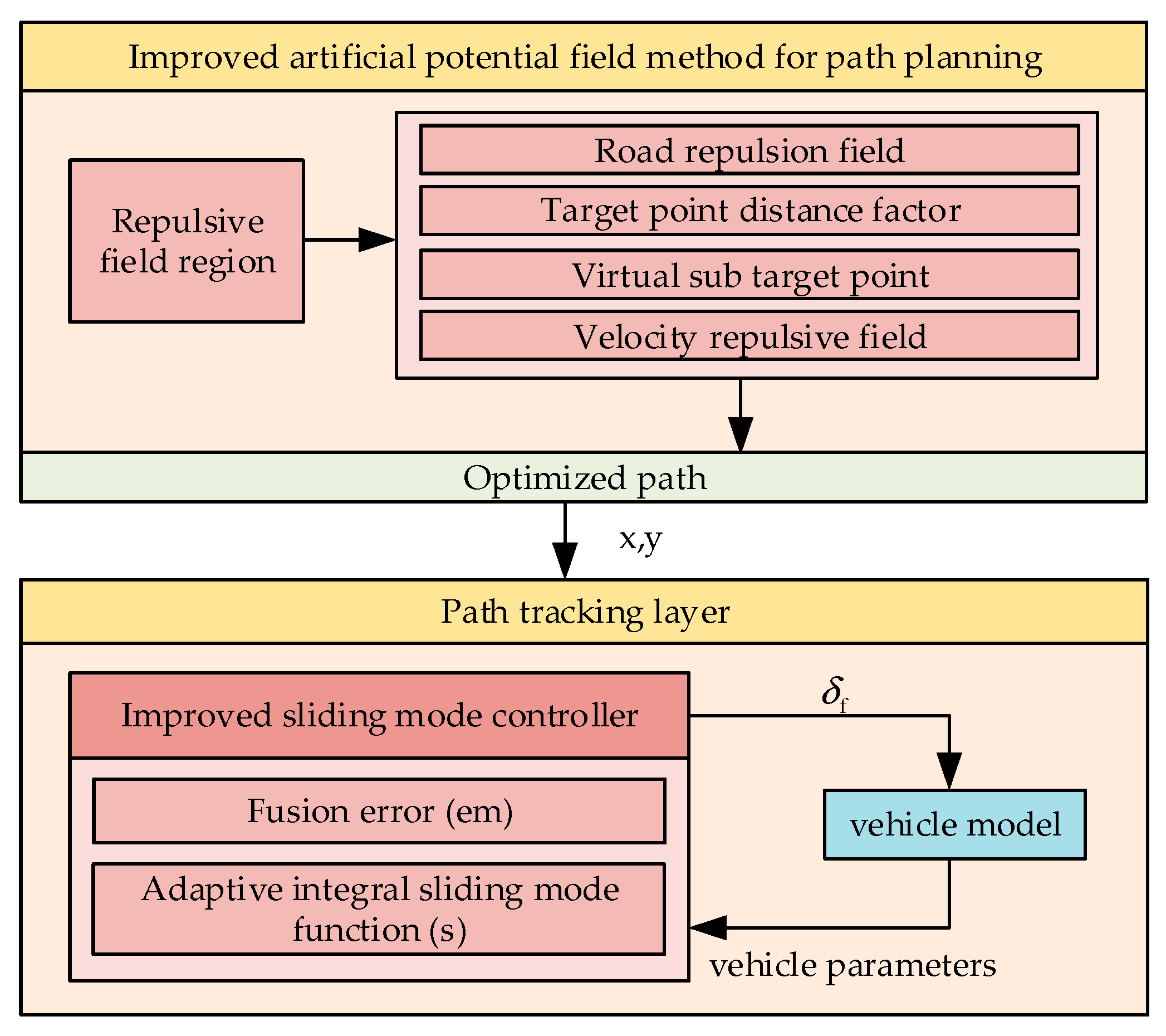
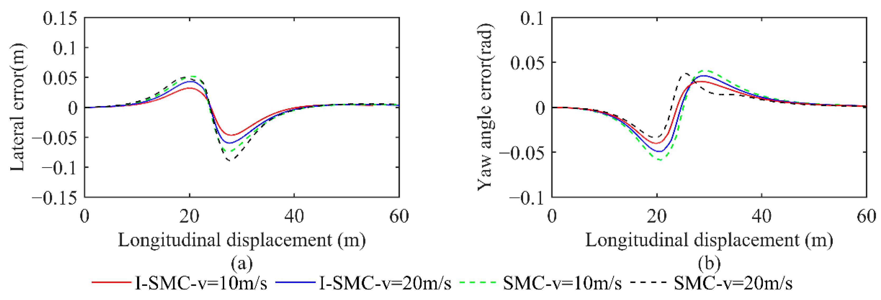
- This study presents an improved sliding mode controller that incorporates error fusion to ensure vehicle driving stability and tracking accuracy, taking into consideration both lateral and heading errors. By utilizing the improved APF algorithm, an optimized path is computed, incorporating vehicle kinematics and dynamics, which is then utilized as input for the lower controller responsible for path tracking. This aims to verify the feasibility of the planned path and evaluate the effectiveness of the enhanced tracking controller.
- 4.
- To verify the effectiveness of path planning and tracking, this study uses the Carsim–Simulink joint simulation platform. The experiment encompasses both static and dynamic scenarios. The static scene involves designing an environment with obstacles and two lanes ahead and utilizing an improved APF method to devise secure routes for vehicles. A vehicle with moving obstacles is placed in the dynamic scene, and the improved APF proposed in this study is used to generate an optimized and safe path for the autonomous vehicle. The experimental results demonstrate that the planned driving path is fully compliant with safety and road constraints, allowing for the vehicle to smoothly reach the endpoint.
2. Path Planning Algorithm
2.1. Traditional APF Algorithm
2.2. Improved APF Method
2.2.1. The Region of Repulsive Field Action
2.2.2. Road Repulsion Field
2.2.3. Target Point Distance Factor
2.2.4. Virtual Sub-Target Point
2.2.5. Velocity Repulsive Field
2.3. Path Optimization Algorithm for a Planned Path
3. Path Tracking Controller
3.1. Vehicle Model
3.2. Design of an Improved SMC Controller
4. Simulation Analysis
4.1. Simulation Analysis of Path Planning
- (1)
- Scenario 1: Changing lanes (static)
- (2)
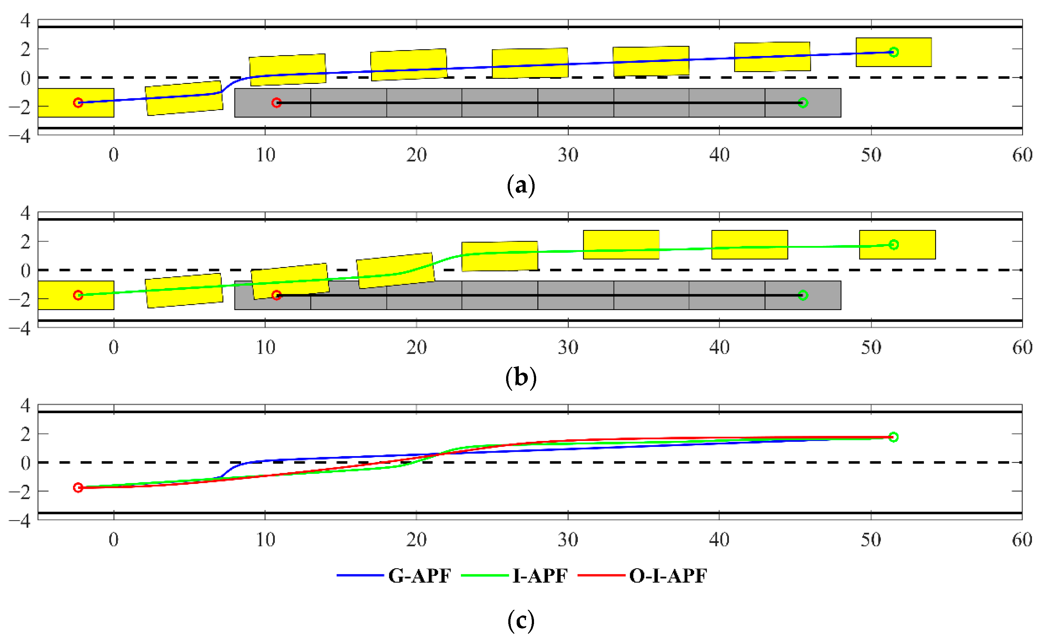
- Scenario 2: Static overtaking
- (3)
- Scenario 3: Dynamic overtaking
4.2. Simulation Analysis of Path Tracking Control
- (1)
- Scenario 1: Changing lanes (static)
- (2)
- Scenario 2: Static overtaking
- (3)
- Scenario 3: Dynamic overtaking
5. Conclusions
Author Contributions
Funding
Data Availability Statement
Conflicts of Interest
References
- Badue, C.; Guidolini, R.; Carneiro, R.V.; Azevedo, P.; Cardoso, V.B.; Forechi, A.; Jesus, L.; Berriel, R.; Paixão, T.M.; Mutz, F.; et al. Self-Driving Cars: A Survey. Expert Syst. Appl. 2021, 165, 113816. [Google Scholar] [CrossRef]
- Xiao, G.; Zhang, H.; Sun, N.; Zhang, Y. Cooperative Link Scheduling for RSU-Assisted Dissemination of Basic Safety Messages. Wirel. Netw. 2021, 27, 1335–1351. [Google Scholar] [CrossRef]
- Wei, Y.; Li, B.; Xu, X.; Wei, M.; Wang, C. Design of Electric Supercharger Compressor and Its Performance Optimization. Processes 2023, 11, 2132. [Google Scholar] [CrossRef]
- Song, Z.; Deng, H. Research on Sensor Optimization Technology of Driverless Vehicle. Front. Comput. Intell. Syst. 2023, 4, 131–137. [Google Scholar] [CrossRef]
- Cai, H.; Xu, X. Lateral Stability Control of a Tractor-Semitrailer at High Speed. Machines 2022, 10, 716. [Google Scholar] [CrossRef]
- Xu, X.; Zhang, L.; Jiang, Y.; Chen, N. Active Control on Path Following and Lateral Stability for Truck–Trailer Combinations. Arab. J. Sci. Eng. 2019, 44, 1365–1377. [Google Scholar] [CrossRef]
- Natan, O.; Miura, J. DeepIPCv2: LiDAR-Powered Robust Environmental Perception and Navigational Control for Autonomous Vehicle. arXiv 2023, arXiv:2307.06647. [Google Scholar]
- Alfred Daniel, J.; Chandru Vignesh, C.; Muthu, B.A.; Senthil Kumar, R.; Sivaparthipan, C.; Marin, C.E.M. Fully Convolutional Neural Networks for LIDAR–Camera Fusion for Pedestrian Detection in Autonomous Vehicle. Multimed Tools Appl. 2023, 82, 25107–25130. [Google Scholar] [CrossRef]
- Zhang, Y.; Zhou, A.; Zhao, F.; Wu, H. A Lightweight Vehicle-Pedestrian Detection Algorithm Based on Attention Mechanism in Traffic Scenarios. Sensors 2022, 22, 8480. [Google Scholar] [CrossRef]
- Shang, Y.; Liu, F.; Qin, P.; Guo, Z.; Li, Z. Research on Path Planning of Autonomous Vehicle Based on RRT Algorithm of Q-Learning and Obstacle Distribution. Eng. Comput. 2023, 40, 1266–1286. [Google Scholar] [CrossRef]
- Yao, J.; Ge, Z. Path-Tracking Control Strategy of Unmanned Vehicle Based on DDPG Algorithm. Sensors 2022, 22, 7881. [Google Scholar] [CrossRef] [PubMed]
- Tian, J.; Wang, Q.; Ding, J.; Wang, Y.; Ma, Z. Integrated Control With DYC and DSS for 4WID Electric Vehicles. IEEE Access 2019, 7, 124077–124086. [Google Scholar] [CrossRef]
- Tian, J.; Yang, M. Hierarchical Control of Differential Steering for Four-in-Wheel-Motor Electric Vehicle. PLoS ONE 2023, 18, e0285485. [Google Scholar] [CrossRef]
- Hou, Y.; Xu, X. High-Speed Lateral Stability and Trajectory Tracking Performance for a Tractor-Semitrailer with Active Trailer Steering. PLoS ONE 2022, 17, e0277358. [Google Scholar] [CrossRef] [PubMed]
- Wang, P.; Liu, Y.; Yao, W.; Yu, Y. Improved A-Star Algorithm Based on Multivariate Fusion Heuristic Function for Autonomous Driving Path Planning. Proc. Inst. Mech. Eng. Part D J. Automob. Eng. 2023, 237, 1527–1542. [Google Scholar] [CrossRef]
- Chen, R.; Hu, J.; Xu, W. An RRT-Dijkstra-Based Path Planning Strategy for Autonomous Vehicles. Appl. Sci. 2022, 12, 11982. [Google Scholar] [CrossRef]
- Zhou, R.; Liu, Y.; Zhang, K.; Yang, O. Genetic Algorithm-Based Challenging Scenarios Generation for Autonomous Vehicle Testing. IEEE J. Radio Freq. Identif. 2022, 6, 928–933. [Google Scholar] [CrossRef]
- Wang, J.; Yuan, X.; Liu, Z.; Tan, W.; Zhang, X.; Wang, Y. Adaptive Dynamic Path Planning Method for Autonomous Vehicle Under Various Road Friction and Speeds. IEEE Trans. Intell. Transp. Syst. 2023, 1–11. [Google Scholar] [CrossRef]
- Qiao, Z.; Tyree, Z.; Mudalige, P.; Schneider, J.; Dolan, J.M. Hierarchical Reinforcement Learning Method for Autonomous Vehicle Behavior Planning. In Proceedings of the 2020 IEEE/RSJ International Conference on Intelligent Robots and Systems (IROS), Las Vegas, NV, USA, 25–29 October 2020; pp. 6084–6089. [Google Scholar]
- Pavel, M.I.; Tan, S.Y.; Abdullah, A. Vision-Based Autonomous Vehicle Systems Based on Deep Learning: A Systematic Literature Review. Appl. Sci. 2022, 12, 6831. [Google Scholar] [CrossRef]
- Baby, T.V.; HomChaudhuri, B. Monte Carlo Tree Search Based Trajectory Generation for Automated Vehicles in Interactive Traffic Environments. In Proceedings of the 2023 American Control Conference (ACC), San Diego, CA, USA, 31 May–2 June 2023; pp. 4431–4436. [Google Scholar]
- Li, H.; Liu, W.; Yang, C.; Wang, W.; Qie, T.; Xiang, C. An Optimization-Based Path Planning Approach for Autonomous Vehicles Using the DynEFWA-Artificial Potential Field. IEEE Trans. Intell. Veh. 2022, 7, 263–272. [Google Scholar] [CrossRef]
- Yao, Q.; Zheng, Z.; Qi, L.; Yuan, H.; Guo, X.; Zhao, M.; Liu, Z.; Yang, T. Path Planning Method With Improved Artificial Potential Field—A Reinforcement Learning Perspective. IEEE Access 2020, 8, 135513–135523. [Google Scholar] [CrossRef]
- Xie, S.; Hu, J.; Bhowmick, P.; Ding, Z.; Arvin, F. Distributed Motion Planning for Safe Autonomous Vehicle Overtaking via Artificial Potential Field. IEEE Trans. Intell. Transp. Syst. 2022, 23, 21531–21547. [Google Scholar] [CrossRef]
- Duan, Y.; Yang, C.; Zhu, J.; Meng, Y.; Liu, X. Active Obstacle Avoidance Method of Autonomous Vehicle Based on Improved Artificial Potential Field. Int. J. Adv. Robot. Syst. 2022, 19, 17298806221115984. [Google Scholar] [CrossRef]
- Feng, S.; Qian, Y.; Wang, Y. Collision Avoidance Method of Autonomous Vehicle Based on Improved Artificial Potential Field Algorithm. Proc. Inst. Mech. Eng. Part D J. Automob. Eng. 2021, 235, 3416–3430. [Google Scholar] [CrossRef]
- Yuan, C.; Weng, S.; Shen, J.; Chen, L.; He, Y.; Wang, T. Research on Active Collision Avoidance Algorithm for Intelligent Vehicle Based on Improved Artificial Potential Field Model. Int. J. Adv. Robot. Syst. 2020, 17, 1729881420911232. [Google Scholar] [CrossRef]
- Tian, J.; Zeng, Q.; Wang, P.; Wang, X. Active Steering Control Based on Preview Theory for Articulated Heavy Vehicles. PLoS ONE 2021, 16, e0252098. [Google Scholar] [CrossRef]
- Li, B.; Zeng, L. Fractional Calculus Control of Road Vehicle Lateral Stability after a Tire Blowout. Mechanics 2021, 27, 475–482. [Google Scholar] [CrossRef]
- Tian, J.; Yang, M. Research on Trajectory Tracking and Body Attitude Control of Autonomous Ground Vehicle Based on Differential Steering. PLoS ONE 2023, 18, e0273255. [Google Scholar] [CrossRef]
- Chen, G.; Zhao, X.; Gao, Z.; Hua, M. Dynamic Drifting Control for General Path Tracking of Autonomous Vehicles. IEEE Trans. Intell. Veh. 2023, 8, 2527–2537. [Google Scholar] [CrossRef]
- Wang, Z.; Sun, K.; Ma, S.; Sun, L.; Gao, W.; Dong, Z. Improved Linear Quadratic Regulator Lateral Path Tracking Approach Based on a Real-Time Updated Algorithm with Fuzzy Control and Cosine Similarity for Autonomous Vehicles. Electronics 2022, 11, 3703. [Google Scholar] [CrossRef]
- Ding, C.; Ding, S.; Wei, X.; Mei, K. Output Feedback Sliding Mode Control for Path-Tracking of Autonomous Agricultural Vehicles. Nonlinear Dyn. 2022, 110, 2429–2445. [Google Scholar] [CrossRef]
- Sun, Z.; Zou, J.; He, D.; Zhu, W. Path-Tracking Control for Autonomous Vehicles Using Double-Hidden-Layer Output Feedback Neural Network Fast Nonsingular Terminal Sliding Mode. Neural Comput. Applic 2022, 34, 5135–5150. [Google Scholar] [CrossRef]
- Ao, D.; Huang, W.; Wong, P.K.; Li, J. Robust Backstepping Super-Twisting Sliding Mode Control for Autonomous Vehicle Path Following. IEEE Access 2021, 9, 123165–123177. [Google Scholar] [CrossRef]
- Sabiha, A.D.; Kamel, M.A.; Said, E.; Hussein, W.M. ROS-Based Trajectory Tracking Control for Autonomous Tracked Vehicle Using Optimized Backstepping and Sliding Mode Control. Robot. Auton. Syst. 2022, 152, 104058. [Google Scholar] [CrossRef]
- Ma, B.; Pei, W.; Zhang, Q. Trajectory Tracking Control of Autonomous Vehicles Based on an Improved Sliding Mode Control Scheme. Electronics 2023, 12, 2748. [Google Scholar] [CrossRef]
- Khatib, O. Real-Time Obstacle Avoidance for Manipulators and Mobile Robots. Int. J. Robot. Res. 1986, 5, 90–98. [Google Scholar] [CrossRef]


| Methods | Merits | Drawbacks |
|---|---|---|
| Based on the safe distance model | Driving safety | Restricted turning radius |
| Algorithm fusion | Real-time performance of path planning | Difficulty in setting the threshold |
| Improvement in the repulsive field | Driving safety, vehicle Stability | Poor adaptability to complex environments |
| Improvement in the gravitational field | Feasibility of path planning, vehicle Stability | Constraints of the traffic environment |
| Multi-condition model | Driving safety | Poor adaptability to complex environments |
| Methods | Merits | Drawbacks |
|---|---|---|
| Hierarchical dynamic drift controller | High tracking accuracy | Poor system stability |
| Discrete LQR | Simple calculations | Weak steering stability |
| Super twisted SMC | Good system stability | Long calculation time |
| Integral terminal SMC | Fast convergence speed | Poor system stability |
| Adaptive integral terminal SMC | Good system stability | Poor tracking accuracy |
| Algorithm | Length (m) | Planning Time (s) | Maximum Curvature (1/m) |
|---|---|---|---|
| G-APF | 60.145 | 0.024 | 0.788 |
| I-APF | 60.286 | 0.011 | 0.201 |
| O-I-APF | 60.009 | 0.012 | 0.033 |
| Algorithm | Length (m) | Planning Time (s) | Maximum Curvature (1/m) |
|---|---|---|---|
| G-APF | 60.491 | 0.019 | 1.164 |
| I-APF | 61.635 | 0.009 | 0.797 |
| O-I-APF | 60.965 | 0.011 | 0.236 |
| Algorithm | Length (m) | Planning Time (s) | Maximum Curvature (1/m) |
|---|---|---|---|
| G-APF | 54.218 | 0.021 | 1.371 |
| I-APF | 54.114 | 0.016 | 0.167 |
| O-I-APF | 53.731 | 0.018 | 0.014 |
| Parameters (Units) | Value |
|---|---|
| Distance from the center of mass to the front axis a (m) | 1.015 |
| Distance from the center of mass to the rear axis b (m) | 1.895 |
| Height of the center of mass h (m) | 0.54 |
| Vehicle mass m (kg) | 1270 |
| Moment of inertia Iz (kg·m2) | 1536 |
| Effective radius of wheel r (m) | 0.325 |
| Front wheel lateral stiffness k1/(N·rad−1) | 56,500 |
| Rear wheel lateral stiffness k2/(N·rad−1) | 66,500 |
Disclaimer/Publisher’s Note: The statements, opinions and data contained in all publications are solely those of the individual author(s) and contributor(s) and not of MDPI and/or the editor(s). MDPI and/or the editor(s) disclaim responsibility for any injury to people or property resulting from any ideas, methods, instructions or products referred to in the content. |
© 2023 by the authors. Licensee MDPI, Basel, Switzerland. This article is an open access article distributed under the terms and conditions of the Creative Commons Attribution (CC BY) license (https://creativecommons.org/licenses/by/4.0/).
Share and Cite
Zhang, Y.; Liu, K.; Gao, F.; Zhao, F. Research on Path Planning and Path Tracking Control of Autonomous Vehicles Based on Improved APF and SMC. Sensors 2023, 23, 7918. https://doi.org/10.3390/s23187918
Zhang Y, Liu K, Gao F, Zhao F. Research on Path Planning and Path Tracking Control of Autonomous Vehicles Based on Improved APF and SMC. Sensors. 2023; 23(18):7918. https://doi.org/10.3390/s23187918
Chicago/Turabian StyleZhang, Yong, Kangting Liu, Feng Gao, and Fengkui Zhao. 2023. "Research on Path Planning and Path Tracking Control of Autonomous Vehicles Based on Improved APF and SMC" Sensors 23, no. 18: 7918. https://doi.org/10.3390/s23187918
APA StyleZhang, Y., Liu, K., Gao, F., & Zhao, F. (2023). Research on Path Planning and Path Tracking Control of Autonomous Vehicles Based on Improved APF and SMC. Sensors, 23(18), 7918. https://doi.org/10.3390/s23187918