
Probabilistic Modeling of Multicamera Interference for Time-of-Flight Sensors

Abstract
:1. Introduction
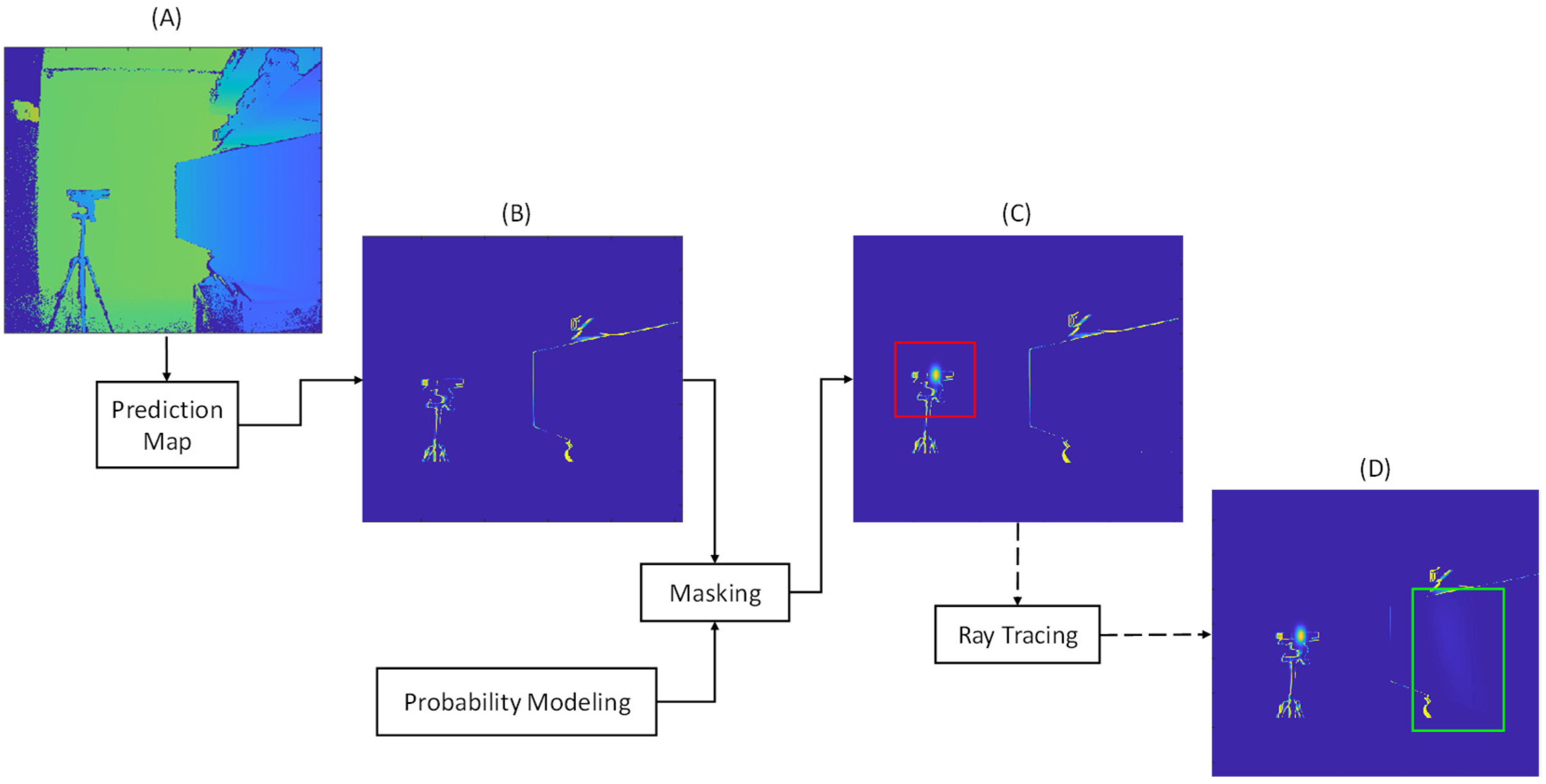
2. Methodology
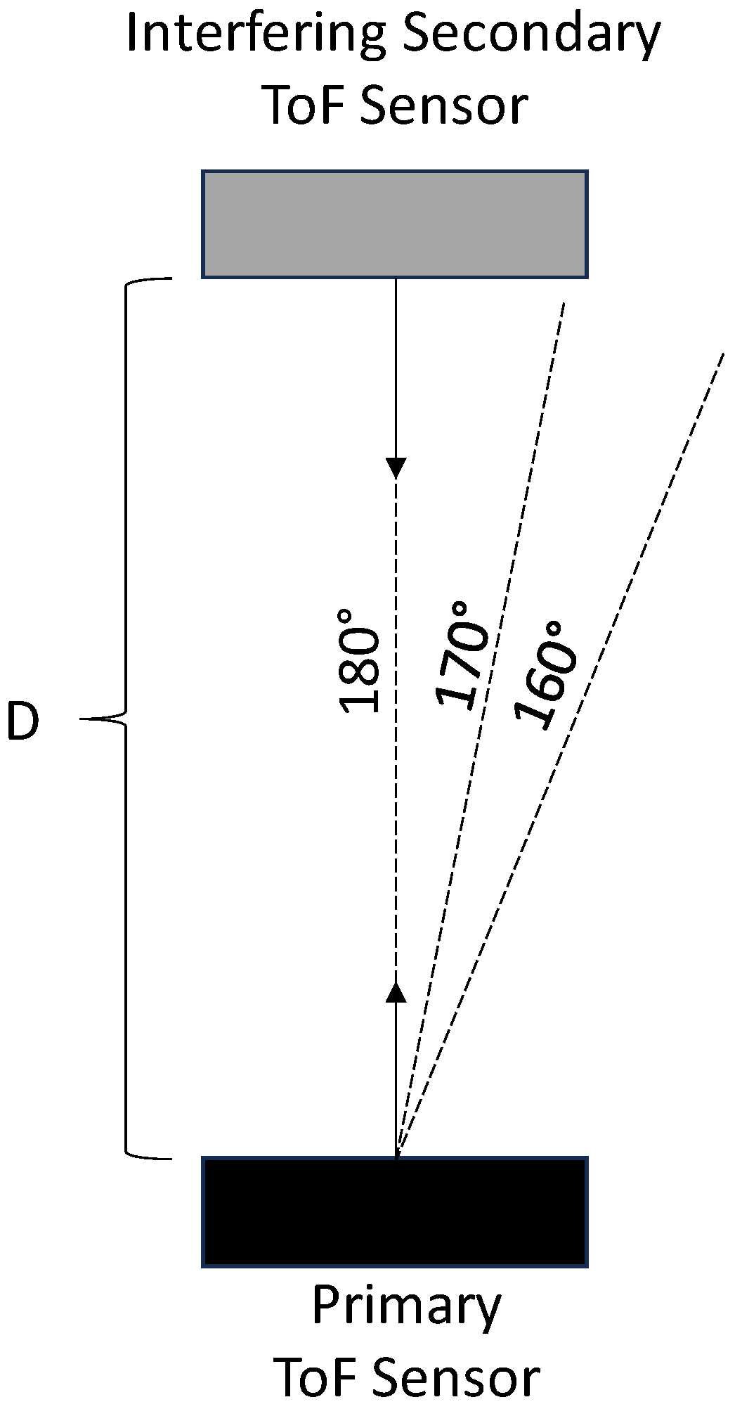
2.1. Multicamera Interference
2.2. Probability Model
2.3. Masking
2.4. Ray Tracing
2.5. Generating Depth Map with Synthetic Multicamera Interference
3. Experiments
3.1. Hardware Configuration
3.2. Performance Metrics
3.3. Direct Interference Experimental Results
3.4. Indirect Interference Experiment Results
3.5. Combined Direct and Indirect Interference Experiment Results
3.6. Non-Zero-Value Pixel Experiment Results
4. Conclusions
Author Contributions
Funding
Institutional Review Board Statement
Informed Consent Statement
Data Availability Statement
Acknowledgments
Conflicts of Interest
References
- Page, D.L.; Fougerolle, Y.; Koschan, A.F.; Gribok, A.; Abidi, M.A.; Gorsich, D.J.; Gerhart, G.R. SAFER vehicle inspection: A multimodal robotic sensing platform. In Unmanned Ground Vehicle Technology VI, Proceedings of the Defense and Security, Orlando, FL, USA, 12–16 April 2004; SPIE: Washington, DC, USA, 2004; Volume 5422, pp. 549–561. [Google Scholar]
- Chen, C.; Yang, B.; Song, S.; Tian, M.; Li, J.; Dai, W.; Fang, L. Calibrate Multiple Consumer RGB-D Cameras for Low-Cost and Efficient 3D Indoor Mapping. Remote Sens. 2018, 10, 328. [Google Scholar] [CrossRef]
- Rodriguez, B.; Zhang, X.; Rajan, D. Synthetically Generating Motion Blur in a Depth Map from Time-of-Flight Sensors. In Proceedings of the 2021 17th International Conference on Machine Vision and Applications (MVA), Aichi, Japan, 25–27 July 2021; pp. 1–5. [Google Scholar]
- Rodriguez, B.; Zhang, X.; Rajan, D. Probabilistic Modeling of Motion Blur for Time-of-Flight Sensors. Sensors 2022, 22, 1182. [Google Scholar] [CrossRef] [PubMed]
- Paredes, J.A.; Álvarez, F.J.; Aguilera, T.; Villadangos, J.M. 3D indoor positioning of UAVs with spread spectrum ultrasound and time-of-flight cameras. Sensors 2018, 18, 89. [Google Scholar] [CrossRef]
- Mentasti, S.; Pedersini, F. Controlling the Flight of a Drone and Its Camera for 3D Reconstruction of Large Objects. Sensors 2019, 19, 2333. [Google Scholar] [CrossRef] [PubMed]
- Jin, Y.-H.; Ko, K.-W.; Lee, W.-H. An Indoor Location-Based Positioning System Using Stereo Vision with the Drone Camera. Mob. Inf. Syst. 2018, 2018, 5160543. [Google Scholar] [CrossRef]
- Pascoal, R.; Santos, V.; Premebida, C.; Nunes, U. Simultaneous Segmentation and Superquadrics Fitting in Laser-Range Data. IEEE Trans. Veh. Technol. 2014, 64, 441–452. [Google Scholar] [CrossRef]
- Shen, S.; Mulgaonkar, Y.; Michael, N.; Kumar, V. Multi-Sensor Fusion for Robust Autonomous Flight in Indoor and Outdoor Environments with a Rotorcraft MAV. In Proceedings of the 2014 IEEE International Conference on Robotics and Automation (ICRA), Hong Kong, China, 31 May–7 June 2014; pp. 4974–4981. [Google Scholar]
- Chiodini, S.; Giubilato, R.; Pertile, M.; Debei, S. Retrieving Scale on Monocular Visual Odometry Using Low-Resolution Range Sensors. IEEE Trans. Instrum. Meas. 2020, 69, 5875–5889. [Google Scholar] [CrossRef]
- Correll, N.; Bekris, K.E.; Berenson, D.; Brock, O.; Causo, A.; Hauser, K.; Okada, K.; Rodriguez, A.; Romano, J.M.; Wurman, P.R. Analysis and Observations from the First Amazon Picking Challenge. IEEE Trans. Autom. Sci. Eng. 2016, 15, 172–188. [Google Scholar] [CrossRef]
- Corbato, C.H.; Bharatheesha, M.; Van Egmond, J.; Ju, J.; Wisse, M. Integrating Different Levels of Automation: Lessons from Winning the Amazon Robotics Challenge 2016. IEEE Trans. Ind. Inform. 2018, 14, 4916–4926. [Google Scholar] [CrossRef]
- Pardi, T.; Poggiani, M.; Luberto, E.; Raugi, A.; Garabini, M.; Persichini, R.; Catalano, M.G.; Grioli, G.; Bonilla, M.; Bicchi, A. A Soft Robotics Approach to Autonomous Warehouse Picking. In Advances on Robotic Item Picking; Springer: Cham, Switzerland, 2020; pp. 23–35. [Google Scholar]
- Shrestha, S.; Heide, F.; Heidrich, W.; Wetzstein, G. Computational imaging with multi-camera time-of-flight systems. ACM Trans. Graph. (ToG) 2016, 35, 1–11. [Google Scholar] [CrossRef]
- Volak, J.; Koniar, D.; Jabloncik, F.; Hargas, L.; Janisova, S. Interference artifacts suppression in systems with multiple depth cameras. In Proceedings of the 2019 42nd International Conference on Telecommunications and Signal Processing (TSP), Budapest, Hungary, 1–3 July 2019; IEEE: New York, NY, USA, 2019. [Google Scholar] [CrossRef]
- Volak, J.; Bajzik, J.; Janisova, S.; Koniar, D.; Hargas, L. Real-Time Interference Artifacts Suppression in Array of ToF Sensors. Sensors 2020, 20, 3701. [Google Scholar] [CrossRef]
- Li, L.; Xiang, S.; Yang, Y.; Yu, L. Multi-camera interference cancellation of time-of-flight (TOF) cameras. In Proceedings of the 2015 IEEE International Conference on Image Processing (ICIP), Quebec City, QC, Canada, 27–30 September 2015; IEEE: New York, NY, USA, 2015. [Google Scholar] [CrossRef]
- Wermke, F.; Meffert, B. Interference model of two time-of-flight cameras. In Proceedings of the 2019 IEEE SENSORS, Montreal, QC, Canada, 27–30 October 2019; IEEE: New York, NY, USA, 2019. [Google Scholar] [CrossRef]
- Castaneda, V.; Mateus, D.; Navab, N. Stereo time-of-flight with constructive interference. IEEE Trans. Pattern Anal. Mach. Intell. 2013, 36, 1402–1413. [Google Scholar] [CrossRef]
- Buttgen, B.; Lustenberger, F.; Seitz, P. Pseudonoise optical modulation for real-time 3-D imaging with minimum interference. IEEE Trans. Circuits Syst. I Regul. Pap. 2007, 54, 2109–2119. [Google Scholar] [CrossRef]
- Buttgen, B.; Seitz, P. Robust optical time-of-flight range imaging based on smart pixel structures. IEEE Trans. Circuits Syst. I Regul. Pap. 2008, 55, 1512–1525. [Google Scholar] [CrossRef]
- Luna, C.; Losada-Gutierrez, C.; Fuentes-Jimenez, D.; Fernandez-Rincon, A.; Mazo, M.; Macias-Guarasa, J. Robust people detection using depth information from an overhead time-of-flight camera. Expert Syst. Appl. 2017, 71, 240–256. [Google Scholar] [CrossRef]
- Horaud, R.; Hansard, M.; Evangelidis, G.; Ménier, C. An overview of depth cameras and range scanners based on time-of-flight technologies. Mach. Vis. Appl. 2016, 27, 1005–1020. [Google Scholar] [CrossRef]
- Mallick, T.; Das, P.; Majumdar, A. Characterizations of noise in Kinect depth images: A review. IEEE Sens. J. 2014, 14, 1731–1740. [Google Scholar] [CrossRef]
- Hansard, M.; Lee, S.; Choi, O.; Horaud, R. Time of Flight Cameras: Principles, Methods, and Applications; Springer Science & Business Media: New York, NY, USA, 2012. [Google Scholar]
- Han, J.; Moraga, C. The influence of the sigmoid function parameters on the speed of backpropagation learning. In International Workshop on Artificial Neural Networks; Springer: Berlin/Heidelberg, Germany, 1995. [Google Scholar] [CrossRef]
- Glassner, A. (Ed.) An Introduction to Ray Tracing; Morgan Kaufmann: Cambridge, MA, USA, 1989. [Google Scholar]
- Ray-Tracing: Generating Camera Rays. Available online: https://www.scratchapixel.com/lessons/3d-basic-rendering/ray-tracing-generating-camera-rays/generating-camera-rays.html (accessed on 13 March 2023).
- A Minimal Ray-Tracer: Rendering Simple Shapes (Spheres, Cube, Disk, Plane, etc.). Available online: https://www.scratchapixel.com/lessons/3d-basic-rendering/minimal-ray-tracer-rendering-simple-shapes/ray-plane-and-ray-disk-intersection.html (accessed on 13 March 2023).
- The Phong Model, Introduction to the Concepts of Shader, Reflection Models and BRDF. Available online: https://www.scratchapixel.com/lessons/3d-basic-rendering/phong-shader-BRDF/phong-illumination-models-brdf.html (accessed on 13 March 2023).
- Phong, B. Illumination for computer generated pictures. Seminal graphics: Pioneering efforts that shaped the field. Graph. Image Process. 1998, 95–101. [Google Scholar] [CrossRef]
- Sarbolandi, H.; Lefloch, D.; Kolb, A. Kinect range sensing: Structured-light versus Time-of-Flight Kinect. Comput. Vis. Image Underst. 2015, 139, 1–20. [Google Scholar] [CrossRef]
- Kolb, A.; Barth, E.; Koch, R.; Larsen, R. Time-of-Flight Cameras in Computer Graphics. Comput. Graph. Forum 2010, 29, 141–159. [Google Scholar] [CrossRef]
- OpenKinect. OpenKinect Project. Available online: https://openkinect.org/wiki/Main_Page (accessed on 25 November 2020).
- Cheng, A.; Harrison, H. Touch Projector. Available online: https://tinyurl.com/bx3pfsxt (accessed on 25 November 2020).
- MATLAB, version 9.9.0. 1467703 (R2020b); The MathWorks Inc.: Natick, MA, USA, 2020.
- Benro. Benro GD3WH 3-Way Geared Head. Available online: https://benrousa.com/benro-gd3wh-3-way-geared-head/ (accessed on 26 April 2021).
- DXL360/S V2 Digital Protractor User Guide. Available online: https://www.roeckle.com/WebRoot/Store13/Shops/62116134/5EB6/6EBD/9A39/4D35/9E28/0A0C/6D12/406A/DXL360S_v2-Dual_Axis_Digital_Protractors.pdf (accessed on 27 April 2021).
- Stasenko, S.; Kazantsev, V. Information Encoding in Bursting Spiking Neural Network Modulated by Astrocytes. Entropy 2023, 25, 745. [Google Scholar] [CrossRef]
- Sara, U.; Akter, M.; Uddin, M. Image quality assessment through FSIM, SSIM, MSE and PSNR—A comparative study. J. Comput. Commun. 2019, 7, 8–18. [Google Scholar] [CrossRef]
- Søgaard, J.; Krasula, L.; Shahid, M.; Temel, D.; Brunnström, K.; Razaak, M. Applicability of existing objective metrics of perceptual quality for adaptive video streaming. In Electronic Imaging, Image Quality and System Performance XIII; Society for Imaging Science and Technology: Springfield, VA, USA, 2016. [Google Scholar]
- Deshpande, R.; Ragha, L.; Sharma, S. Video quality assessment through PSNR estimation for different compression standards. Indones. J. Electr. Eng. Comput. Sci. 2018, 11, 918–924. [Google Scholar] [CrossRef]
- Huynh-Thu, Q.; Ghanbari, M. Scope of validity of PSNR in image/video quality assessment. Electron. Lett. 2008, 44, 800–801. [Google Scholar] [CrossRef]
- Hore, A.; Ziou, D. Image quality metrics: PSNR vs. SSIM. In Proceedings of the 2010 20th International Conference on Pattern Recognition, Istanbul, Turkey, 23–26 August 2010; pp. 2366–2369. [Google Scholar] [CrossRef]
- Lu, Y. The level weighted structural similarity loss: A step away from MSE. Proc. AAAI Conf. Artif. Intell. 2019, 33, 9989–9990. [Google Scholar] [CrossRef]


| Symbol | Description |
|---|---|
| The depth map in 2D matrix of pixels with dimensions | |
| The prediction map in 2D matrix of pixels with dimensions | |
| The probability map in 2D matrix of pixels with dimensions | |
| The sigmoid function probability of a pixel being a zero-value pixel | |
| The peak probability value for the sigmoid function | |
| The slope of the sigmoid function | |
| The location of the midpoint of the sigmoid function in pixels | |
| The origin and physical location of the primary ToF sensor | |
| The virtual physical location of a pixel of the primary ToF sensor | |
| The vector associated with a pixel of the ToF sensor | |
| The physical location of the interfering secondary ToF sensor | |
| The virtual physical location of a pixel of the interfering secondary ToF sensor | |
| The vector associated with a pixel of the interfering secondary ToF sensor | |
| The parametric distance between the interfering secondary ToF sensor and an intersection point on a target surface | |
| The physical location of an intersection point on a target surface for a pixel vector from the interfering secondary ToF sensor | |
| The parametric distance between the primary ToF sensor and an intersection point on a target surface | |
| The physical location of an intersection point on a target surface for a pixel vector from the primary ToF sensor | |
| The modified probability value for a pixel from the Phong model for specular reflection and diffusion | |
| The Phong model diffusion, specular reflection, and specular exponential coefficients | |
| , associated with the primary ToF sensor | |
| The physical location of a point on a target surface | |
| The surface normal of a target surface |
| Position Angle = 180° | Axis 1 | Axis 2 | ||||
| Distance: | A | B | C | A | B | C |
| 1.0 m | 1 | −0.3516 | 10.020 | 1 | −0.1912 | 13.870 |
| 1.2 m | 1 | −0.2312 | 9.382 | 1 | −0.2217 | 11.640 |
| 1.4 m | 1 | −0.1931 | 9.003 | 1 | −0.2249 | 9.961 |
| 1.6 m | 1 | −0.3300 | 7.328 | 1 | −0.2912 | 8.608 |
| Position Angle = 170° | Axis 1 | Axis 2 | ||||
| Distance: | A | B | C | A | B | C |
| 1.0 m | 1 | −0.2504 | 9.672 | 1 | −0.2004 | 12.170 |
| 1.2 m | 1 | −0.2489 | 8.188 | 1 | −0.2812 | 10.410 |
| 1.4 m | 1 | −0.3560 | 7.063 | 1 | −0.2869 | 9.596 |
| 1.6 m | 1 | −0.3691 | 6.824 | 1 | −0.2548 | 9.378 |
| Position Angle = 160° | Axis 1 | Axis 2 | ||||
| Distance: | A | B | C | A | B | C |
| 1.0 m | 1 | −0.2093 | 10.010 | 1 | −0.2081 | 14.190 |
| 1.2 m | 1 | −0.2560 | 8.302 | 1 | −0.2099 | 12.230 |
| 1.4 m | 1 | −0.3097 | 7.346 | 1 | −0.2649 | 10.370 |
| 1.6 m | 1 | −0.2288 | 7.103 | 1 | −0.1845 | 10.700 |
| Position Angle = 180° | |||
| Distance: | RMSE | PSNR (dB) | SSIM |
| 1.0 m | 0.0668 | 23.4984 | 0.8733 |
| 1.2 m | 0.0695 | 23.1541 | 0.9037 |
| 1.4 m | 0.0637 | 23.9189 | 0.8920 |
| 1.6 m | 0.0584 | 24.6660 | 0.9286 |
| Position Angle = 170° | |||
| Distance: | |||
| 1.0 m | 0.0564 | 24.9814 | 0.9079 |
| 1.2 m | 0.0534 | 25.4517 | 0.9084 |
| 1.4 m | 0.0547 | 25.2334 | 0.9147 |
| 1.6 m | 0.0672 | 23.4590 | 0.9084 |
| Position Angle = 160° | |||
| Distance: | |||
| 1.0 m | 0.0582 | 24.7000 | 0.9044 |
| 1.2 m | 0.0618 | 24.1834 | 0.8964 |
| 1.4 m | 0.0616 | 24.2029 | 0.9061 |
| 1.6 m | 0.0787 | 22.0837 | 0.8642 |
| Pivot Angle: | RMSE | PSNR (dB) | SSIM |
|---|---|---|---|
| 15° | 0.0496 | 26.0831 | 0.9440 |
| 20° | 0.0397 | 28.0190 | 0.9456 |
| 25° | 0.0227 | 32.8678 | 0.9462 |
| 30° | 0.0127 | 17.9422 | 0.7897 |
| Position Angle = 30° | ||||
| Distance: | 0.8 m | 1.0 m | 1.2 m | 1.4 m |
| Error: | 1.50 mm | 1.10 mm | 0.09 mm | 0.08 mm |
| Position Angle = 45° | ||||
| Distance: | 0.8 m | 1.0 m | 1.2 m | 1.4 m |
| Error: | 0.09 mm | 0.06 mm | 0.06 mm | 0.04 mm |
| Position Angle = 60° | ||||
| Distance: | 0.8 m | 1.0 m | 1.2 m | 1.4 m |
| Error: | 3.00 mm | 0.07 mm | 0.06 mm | 0.05 mm |
Disclaimer/Publisher’s Note: The statements, opinions and data contained in all publications are solely those of the individual author(s) and contributor(s) and not of MDPI and/or the editor(s). MDPI and/or the editor(s) disclaim responsibility for any injury to people or property resulting from any ideas, methods, instructions or products referred to in the content. |
© 2023 by the authors. Licensee MDPI, Basel, Switzerland. This article is an open access article distributed under the terms and conditions of the Creative Commons Attribution (CC BY) license (https://creativecommons.org/licenses/by/4.0/).
Share and Cite
Rodriguez, B.; Zhang, X.; Rajan, D. Probabilistic Modeling of Multicamera Interference for Time-of-Flight Sensors. Sensors 2023, 23, 8047. https://doi.org/10.3390/s23198047
Rodriguez B, Zhang X, Rajan D. Probabilistic Modeling of Multicamera Interference for Time-of-Flight Sensors. Sensors. 2023; 23(19):8047. https://doi.org/10.3390/s23198047
Chicago/Turabian StyleRodriguez, Bryan, Xinxiang Zhang, and Dinesh Rajan. 2023. "Probabilistic Modeling of Multicamera Interference for Time-of-Flight Sensors" Sensors 23, no. 19: 8047. https://doi.org/10.3390/s23198047
APA StyleRodriguez, B., Zhang, X., & Rajan, D. (2023). Probabilistic Modeling of Multicamera Interference for Time-of-Flight Sensors. Sensors, 23(19), 8047. https://doi.org/10.3390/s23198047