Abstract
Piezoelectric vibration sensors (PVSs) are widely applied to vibration detection in aerospace engines due to their small size, high sensitivity, and high-temperature resistance. The precise prediction of their remaining useful life (RUL) under high temperatures is crucial for their maintenance. Notably, digital twins (DTs) provide enormous data from both physical structures and virtual models, which have potential in RUL predictions. Therefore, this work establishes a DT framework containing six modules for sensitivity degradation detection and assessment on the foundation of a five-dimensional DT model. In line with the sensitivity degradation mechanism at high temperatures, a DT-based RUL prediction was performed. Specifically, the PVS sensitivity degradation was described by the Wiener–Arrhenius accelerated degradation model based on the acceleration factor constant principle. Next, an error correction method for the degradation model was proposed using real-time data. Moreover, parameter updates were conducted using a Bayesian method, based on which the RUL was predicted using the first hitting time. Extensive experiments on distinguishing PVS samples demonstrate that our model achieves satisfying performance, which significantly reduces the prediction error to 8 h. A case study was also conducted to provide high RUL prediction accuracy, which further validates the effectiveness of our model in practical use.
1. Introduction
Aeroengines for aircraft must balance requirements of high power, lightweight, safety, reliability, and continuity of service [1]. While working in harsh environments, the high-speed rotation inevitably causes vibration and, thus, component degradation. Therefore, detecting and reducing vibration are highlighted. Nevertheless, considering the complexity of internal combustion, the elimination of vibration based on the working principle of aeroengines remains challenging [2]. Therefore, only when the vibration of an aeroengine is measured in real-time can the safety of an aircraft be maintained to the greatest extent [3]. The exploitation of piezoelectric vibration sensors (PVSs) provides one approach to this challenge, due to the stability of their long-term operation under high-temperature conditions [4]. As an example, the CFM56 turbofan engine in the Boeing 737 uses PVSs to identify working states in every individual rotational cycle [5]. Studies are ongoing that aim to develop PVS-based methods for aeroengine condition monitoring.
PVSs are highly significant, and improvements in their reliability are paramount [6,7]. Despite advances in the optimization of their materials and structure, the risk of PVS failure due to the effect of thermo-mechanical coupling, restricted to aeroengine working conditions, still exists [8,9]. As a result, remaining useful life (RUL) prediction, on the basis of PVS degradation assessments, was proposed [10]. Current RUL prediction approaches are generally carried out based on either physical failure patterns or data-driven models. With respect to the degradation of PVSs, they have two main limitations. First, the stress distribution in working PVSs is so complex that the application of the physical failure model fails to perform its working state precisely [11]. Second, in line with the confidentiality principle, the onboard data for PVS malfunction characterization is currently inaccessible. For this reason, accurate data-driven PVS degradation modeling remains absent.
More recently, advances in DT gave rise to opportunities to develop RUL prediction methods. Theoretically, a DT is a digital representation of a physical structure that comprises the selected elements and dynamics within its lifespan, which bridges the gap between the virtual and the real world [12,13]. Based on real-time interactions between virtual models and physical structures, the degradation of a target system, especially a sensing device, can be derived and evaluated effectively. Recently, Feng et al. developed a DT-driven intelligent method to assess gear surface degradation under harsh conditions [14]. Jafari and Khadim et al. devised a DT-based state-estimation method to model the dynamics of hydraulically actuated machinery [15]. Byun proposed a DT framework for battery-state prediction, which improves the accuracy of battery management [16]. Don et al. used vibration data for the fatigue-life prognosis of a vertical oil well drill string [17]. Accordingly, by modeling the mechanical structure, working principle, and degradation mechanism, a DT methodology is capable of digitizing complicated electromechanical equipment [18]. Despite the complex working conditions of PVSs, a DT solution can be applied to RUL predictions.
The use of DT in PVS degradation models is, however, still limited because of the primary challenge of establishing high-fidelity physical and virtual twins. Each PVS, which consists of multiple components, has multiple properties that vary under different conditions. A DT model cannot be built until synchrony between the physical structure and the digital model is achieved. Furthermore, an accurate RUL prediction approach is also expected. The operational process inevitably deteriorates the status of a PVS, and the available information has to be specifically adapted and used to complete the degradation assessment.
The objective of this work is to propose a PVS-specific DT method for the task of RUL prediction. We focus here on establishing a precise DT model to characterize the environment and state of a PVS. Our method aims to predict the RUL in a novel way by using the data of both working and testing conditions.
The contribution of this work is threefold and summarized as follows:
A novel DT framework is designed and deployed based on the working principle of PVSs. The scheme paves the way for DT-based modeling of similar devices.
A RUL prediction is performed using both historical degradation data and real-time degradation data, and provides accurate RUL prediction results for the PVS.
Experiments are conducted to validate the working performance on a set of PVS samples. The experimental results show that our method is superior in RUL prediction tasks under different conditions.
2. Prerequisite
2.1. PVS-Specific DT
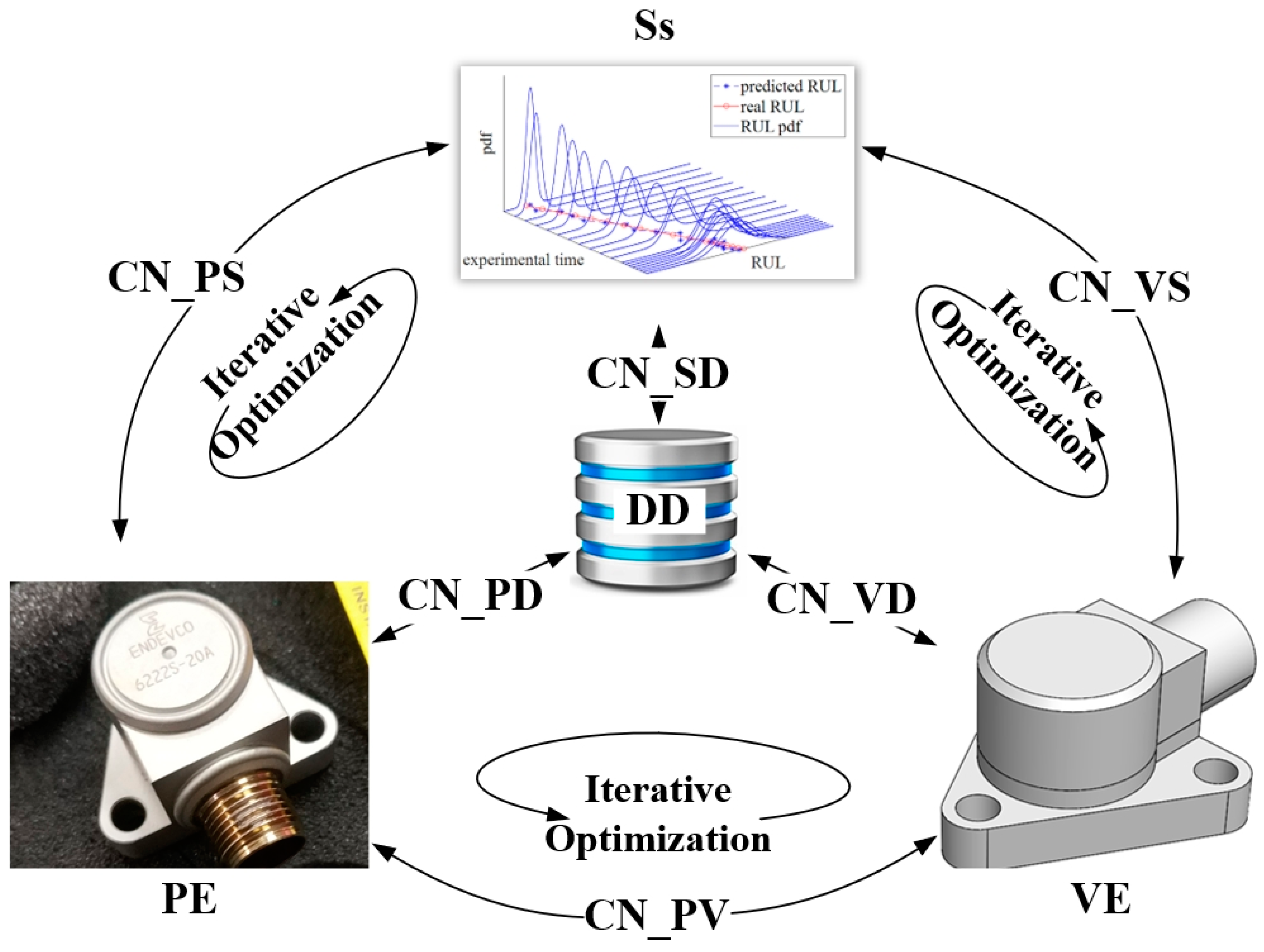
During the task of vibration detection [19], a PVS is capable of converting vibrations into an electrical signal via the piezoelectric effect. Similar to a collection of sensing devices [20,21,22], a PVS has a complex structure and harsh working conditions. In this work, a PVS-specific DT framework is established based on a five-dimensional DT architecture. The standard five-dimensional DT model was originally proposed by Tao et al. for the description of complex systems [23,24]. The architecture of a typical five-dimension DT model is presented in Figure 1. A five-dimensional DT model covers not only the physical entities, virtual entities, and connections between them, but also the data and services; see Equation (1) [25].
where is the five-dimension DT model; represents the physical entity; is the virtual equipment; indicates the services for PE and VE; refers to DT data; and is the connection among other parts.
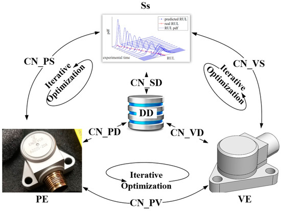
Figure 1.
Architecture of five-dimension DT model.
More details of the PVS-specific DT model are presented below.
2.1.1. Physical Entity (PE)
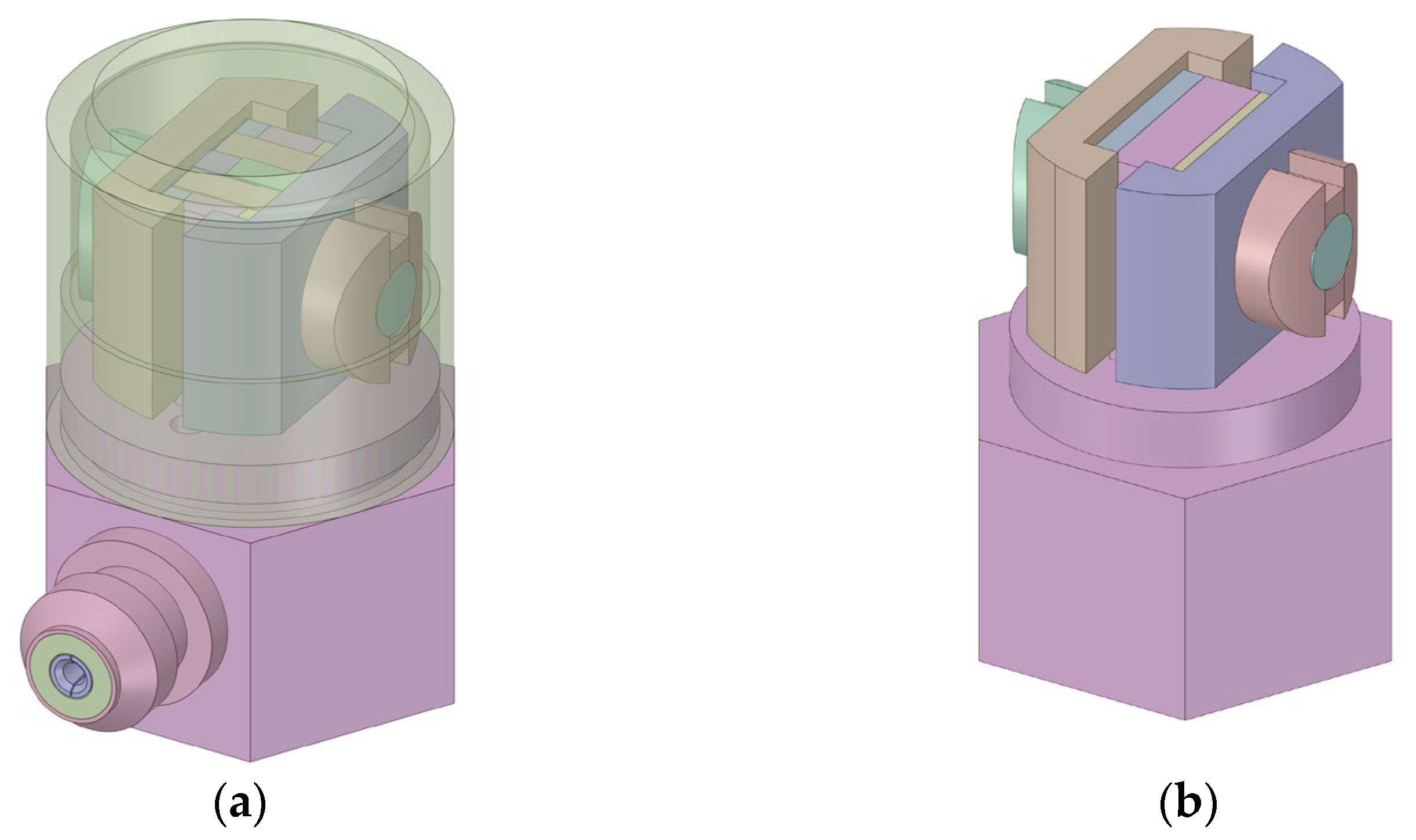
The PE of the PVS-specific DT model contains the body of the PVS, its components, and the attached measuring devices [23]. Generally, the PVS can be categorized as a shear type and a compression type, which are respectively subjected to shear stress and compressive stress. Figure 2 shows the structure of both types, which consist of similar components but have distinguishing mechanical characteristics. For both types, a PVS is composed of a casing, a base, a connector, two mass blocks, a pre-load screw-pair, two piezoelectric strips, two conducting strips, and an insulating strip. The pre-load is applied to the mass block, the piezoelectric strip, and the conducting strip, which are assembled with the pre-load screw-pair. Notably, the pre-load direction of the compression-type PVS is consistent with the sensitive direction, while that of the shear type is vertical to the sensitive direction. In addition, the measuring device is used for the PVS test, which contains a charge amplifier, signal acquisition equipment, calibration equipment, and temperature sensing elements.
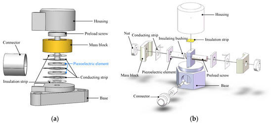
Figure 2.
The main structure types of PVSs: (a) shear-type PVS and (b) compression-type PVS.
2.1.2. Virtual Equipment (VE)
The VE is a high-fidelity digital model of PE, which reproduces geometries, physical properties, behaviors, and rules of PE in the virtual world [23]. In this work, the VE of a PVS is subdivided into three models as follows
where is the vibration–electrical conversion model, is the simulation model for mechanical and thermal stress characterization, and is the RUL prediction model.
Vibration–Electrical Conversion Model : The critical function of a PVS is vibration–electrical signal conversion. We use sensitivity to describe the relationship between output and input, as presented in Equation (3).
where represents the PVS sensitivity with the dimension of , is the output charge () at time , and is the input vibrating acceleration () at time .
Precisely, the vibration is sensed via charge signals and converted into electrical voltages using a charge amplifier. Then, with filters applied, a sinusoidal waveform is obtained.
where is the half peak of the output voltage () at time and is the conversion factor of the charge amplifier ().
Substituting Equation (3) into Equation (4), the vibrating acceleration is computed as:
Aiming at measuring the PVS sensitivity, a set of vibration signals are sent to two PVSs, i.e., a measurement standard PVS and a target PVS. According to Equation (5), for both PVSs, we have:
which can be transformed into:
where , , and are parameters of the measurement standard, while and can be measured during testing. The sensitivity of the target PVS is thus determined.
Simulation Model with simplified structure: As pointed out in the Introduction, the working environment of a PVS is severe, which results in complex mechanical and thermal stress. The simulation model is performed using finite element analysis (FEA) to reproduce the working status of a PVS. The natural frequency is exploited to demonstrate the vibration property. Notably, the simulation model is built based on structure modeling. We shall thus investigate the significance of each component and simplify the structure of PVS to facilitate the simulation.
Using the simulation analysis shown in Appendix A, the simplified structure of a shear-type PVS is derived and presented in Figure 3. A comparison between the simplified structure and the original compression PVS is given in Figure 4.
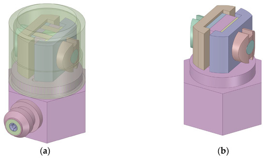
Figure 3.
Structure of a shear-type PVS used in the simulation model: (a) original and (b) simplified.
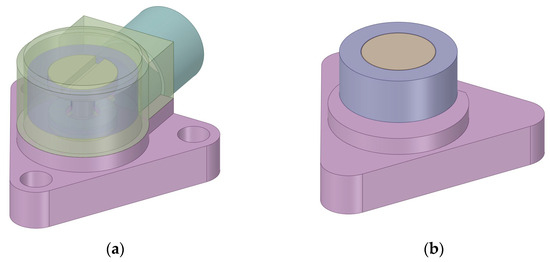
Figure 4.
Structure of the compression PVS used in the simulation model: (a) original and (b) simplified.
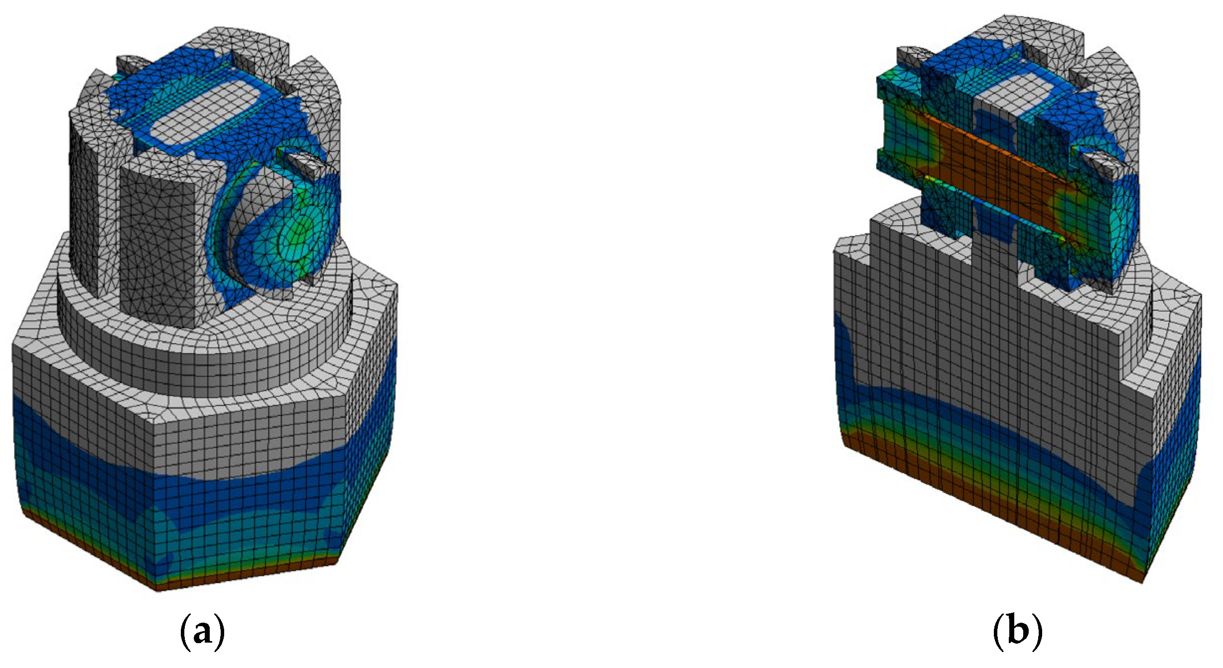
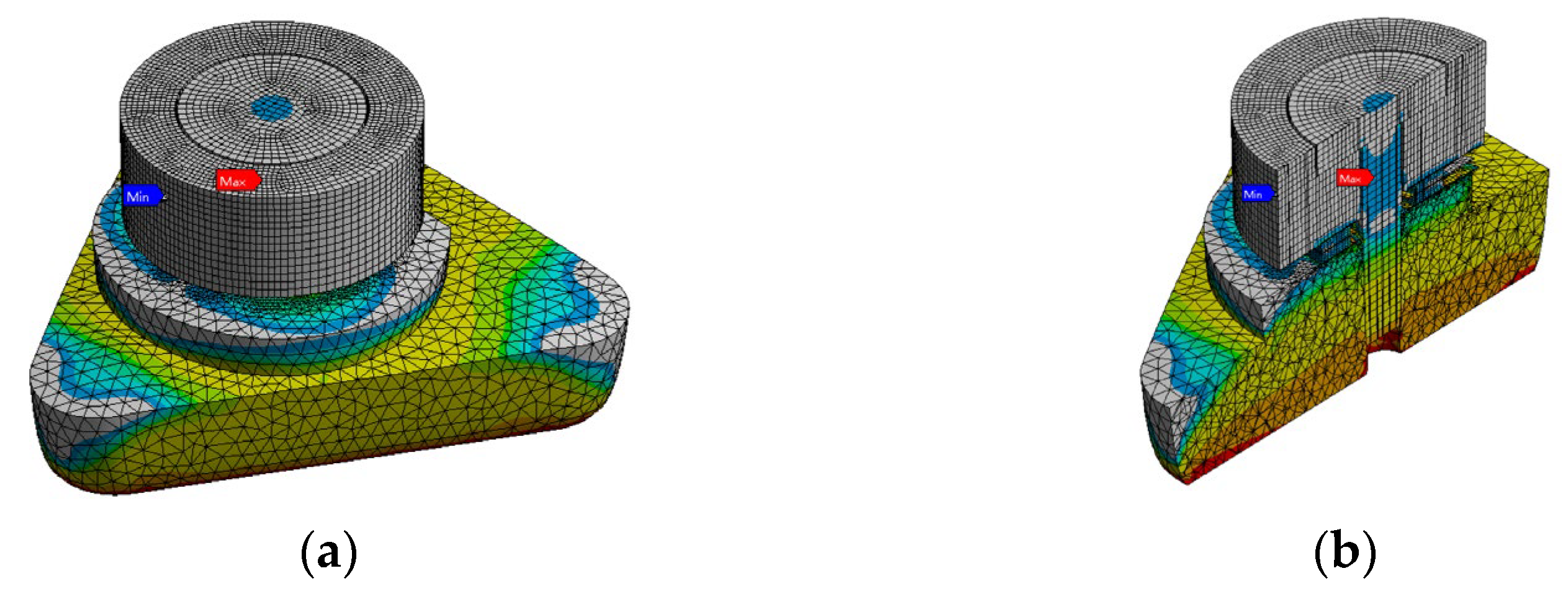
Using a simplified structure, a more efficient stress model is thus built for simulation. With respect to natural-frequency-based simulation, primary attention is paid to the stress simulation of piezoelectric elements. Considering that the stress of piezoelectric sheets is transmitted from the pre-load structure to its surfaces, we perform a more fine-grained meshing on the contact surfaces, which aims to maintain consistency on both sides. Furthermore, considering the working environment and the PVS thermal conductivity, the simulation temperature is set within the range of 423.15 K and 493.15 K. Examples of simulation outcomes for both shear PVS and compression PVS at the temperature of 473.15 K are presented in Figure 5 and Figure 6.

Figure 5.
Stress distribution simulation results for shear PVS: (a) overall view and (b) sectional view.

Figure 6.
Stress distribution simulation results for compression PVS: (a) overall view and (b) sectional view.
RUL Prediction Model : The RUL prediction model is composed of a degradation unit, an accelerated degradation unit, and a life prediction unit.
The degradation of PVS is characterized by a stochastic process. For one thing, sensitivity degradation is performed in a non-monotonic and non-linear fashion, which is affected by thermal stresses and varies for every single PVS. For another, in the context of PVS RUL prediction, a large amount of sensitivity degradation data is unavailable, especially for consistent working conditions. For this reason, a stochastic process, with remarkable statistical properties and mathematical fitting, is used not just to describe a non-monotonic and non-linear trend but also to address the issue of a small sample [26,27]. A non-linear Wiener stochastic process is used to describe PVS sensitivity degradation.
Furthermore, accelerated degradation denotes the relation between performance deterioration and applied stress. Following the idea of [28], accelerated degradation carried out in a stochastic process is capable of resolving inconsistent degradation under different thermal stress conditions. The Arrhenius model, which relates to thermal stress modeling, is used. The acceleration factor constant principle (AFCP) is applied to the accelerated degradation modeling design and parameter determination. In such a manner, a Wiener–Arrhenius sensitivity accelerated degradation process is also developed.
Parameters of both units can be finetuned in line with real-time sensitivity degradation with PVS calibration. All degradation data are analyzed to obtain a degradation mechanism, which is applied to PVS RUL prediction. The degradation data generation and RUL prediction are conducted in the framework of Python 3.9.0. The approaches for each process are depicted in detail in Section 4.
2.1.3. Services (Ss)
Following the idea of Tao et al., Ss involves the optimization of PE whilst adjusting VE to sustain its performance with PE [23]. With respect to the PVS-specific DT model, Ss contains external device control and operation, model management and application, data storage and processing, visualization, etc.
2.1.4. DT Data (DD)
DD contain the data from PE, VE, and Ss domain-specific knowledge as well as their fusion [23]. PE data concerns data on design, operation, and testing. More specifically, test data come from both historical tests and real-time tests of PVS. VE data relate to the model establishment, simulation, and computation. Ss data are collected during all service procedures. The fusion data is the integration of all the above data.
2.1.5. Connections (CNs)
A CN is devised for the interconnection of all other parts, based on which six bidirectional connections, i.e., Ss and DD, PE and DD, VE and DD, PE and Ss, VE and Ss, and PE and VE, are respectively built [23]. In RUL prediction, the connection between PE and DD sets a foundation for state monitoring. The interaction among various connecting parts is utilized to recall historical PVS data, identify current degradation, and obtain real-time processing results. In certain cases, human intervention is also involved with the connection, especially for PE adjustment and system initialization.
2.2. Failure Modes of PVS
An abnormality that characterizes sensor failure is abnormal output, which is also true for the failure of a PVS. A vibration is delivered from the base to the pre-loaded structure and further reaches the piezoelectric strip. The electrical charges are thus generated and sent out via a signal transmission wire. In this way, a sensor malfunction results wherever a problem arises. In general, failure modes of PVS contain structure damage, electrical faults, and sensitivity out of tolerance. Currently, the widely used PVSs are made of stainless steel and tungsten of high rigidity and stability, which are capable of resisting mechanical destruction. Moreover, the reliability of electrical components can be established with design assurance and processing assurance. By contrast, sensitivity degradation plays a pivotal role in RUL prediction results. Considering that a PVS is a piezoelectric-based sensing device, piezoelectric crystals tend to degrade under the condition of intensive stress. Recent publications reveal crack diffusion and phase transitions of piezoelectric elements caused by stress application [29,30,31]. Furthermore, owing to the disparity in the thermal expansion coefficient, a high environmental temperature also leads to a stress increase in a PVS.
As an example, a shear-type PVS works under high-temperature conditions for hundreds of hours, which results in sensitivity out of tolerance. After disassembling components, cracks on a piezoelectric strip are observed. Either a piezoelectric element malfunction or a pre-load manner can induce this failure. For this reason, the sensitivity has to be calibrated in time, based on which the degradation trend can be documented for working state analysis.
3. Methodology
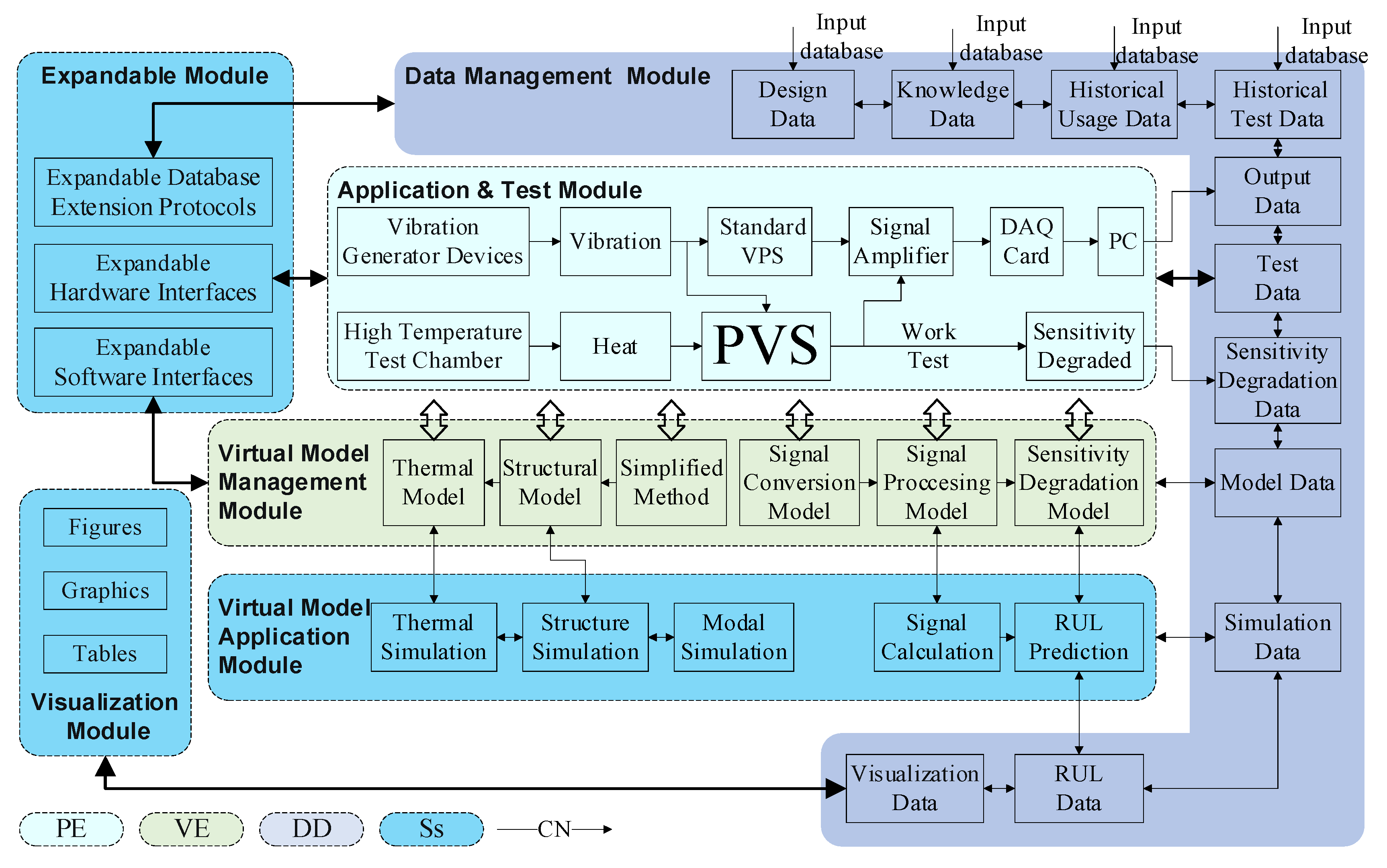
Aiming at predicting the RUL of PVS, a DT-driven sensitivity degradation assessment framework is established. On the one hand, this framework involves all five dimensions in the proposed PVS-specific DT model. On the other hand, the RUL prediction method has six basic modules that present the real-time PVS status, deal with both physical and virtual working conditions, diagnose sensitivity degradation, and provide users with prediction results. The architecture of the proposed method is shown in Figure 7. Each module in this method is described in detail below.
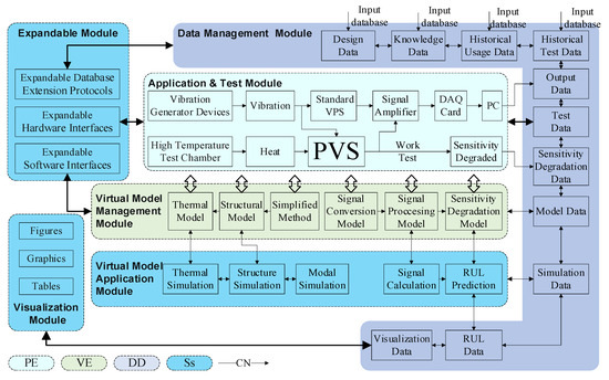
Figure 7.
The architecture of a DT for RUL prediction.
Application and test module: The application and test module mainly contain the PE setup for PVS working and testing and the VE application for modeling and simulation, together with Ss, DD, and CN generated and utilized during operation. The PVS sensitivity measurement is carried out in the application and test module. This module concerns a target PVS, measurement devices, environmental devices, and the sensitivity degradation test scheme. For the PVS test, a measurement standard, a charge amplifier, a DAQ card, and a host computer are used as measurement devices. In addition, the environmental devices consist of a vibration exciter, a power amplifier, a waveform generator for vibration signal generation, and a high-temperature chamber for simulating severe working environments.
Virtual model management module: The virtual model refers to all models in VE, i.e., a vibration–electrical conversion model, a simulation model, and a degradation model. The virtual model management module is designed as an auxiliary to the application and test modules, which provides a more accurate description of PE in virtual space for RUL prediction.
Virtual model application module: This module relates to Ss and CN and bridges the gap among PE, VE, and DD. Specifically, not only the thermal, structural, and modal simulations but also the data computations are incorporated in the virtual model application module. More details of the RUL prediction algorithm are presented in Section 4.
Data management module: The data management module supports the interactions among different modules. In the proposed method, the measurement and sensitivity degradation data are collected in the application and test modules; the model information is conveyed from the virtual model management module, and the simulation and prediction results are generated in the virtual model application module. All data are stored in the database of DD.
Expandable module: The expandable module is responsible for the expansion of PE devices, VE models, Ss protocols, and DD datasets. The method upgrade is also performed in this module.
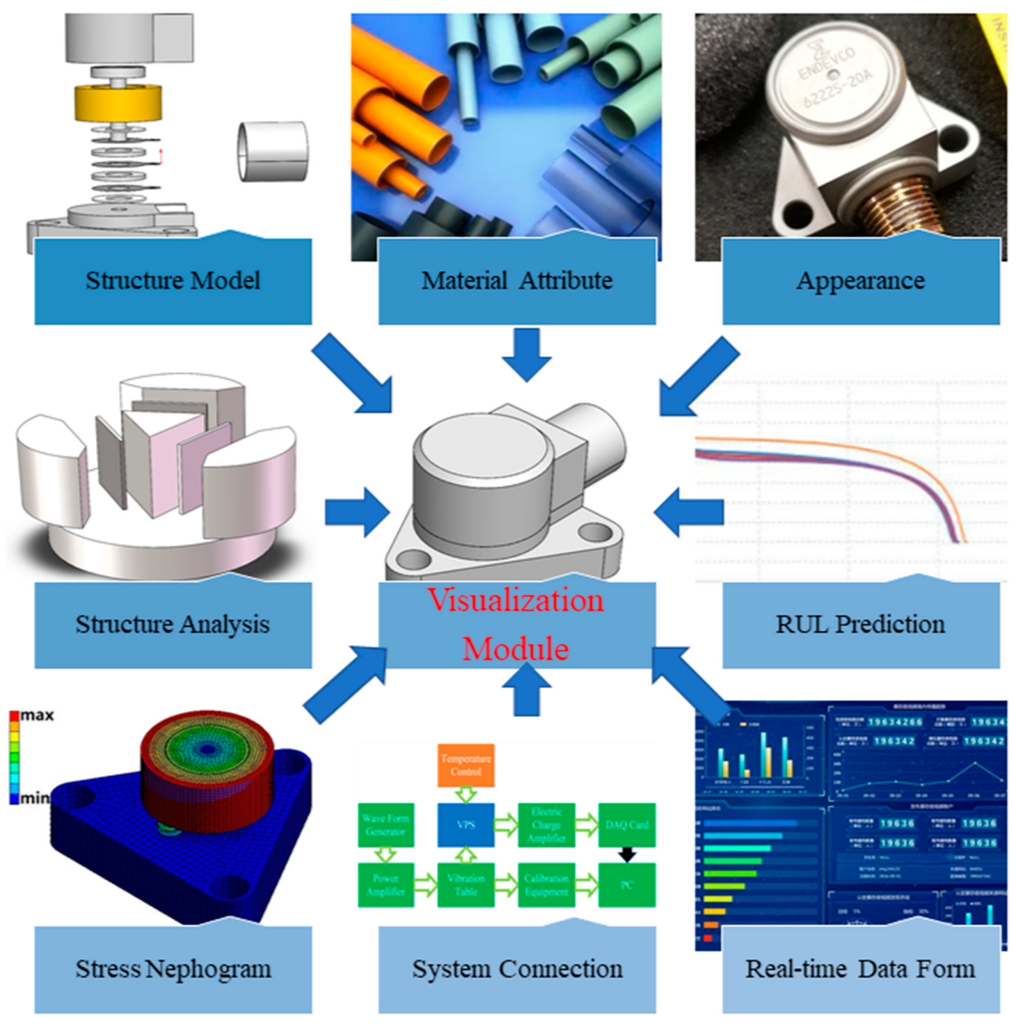
Visualization module: The visualization module is one branch of Ss that illustrates the information of each module. The interface of the visualization module is shown in Figure 8.

Figure 8.
Interface of the visualization module.
4. RUL Prediction Algorithm
In the virtual model application module, two processing steps can be distinguished when performing RUL prediction: sensitivity degradation modeling and life prediction. Specifically, sensitivity degradation is further characterized by the acceleration factor constant principle (AFCP), while the life prediction is conducted using a dynamic correction mechanism.
4.1. Sensitivity Degradation Modeling
From the description above, PVS sensitivity degradation is generally influenced by thermal stresses under working conditions, which is defined as accelerated degradation. To start with, considering the randomness and individual differences in each sensing device, sensitivity degradation is performed in a stochastic process. A non-linear Wiener process is used to model non-monotonical and non-linear degradation data [27]. First, define the sensitivity degradation at time as:
and
With a power–time function , the stochastic sensitivity degradation process is transformed to:
where λ is a drift coefficient that denotes individual differences among the same batch samples; refers to the diffusion coefficient; is standard Brownian motion, and is used for time scaling. For each , the correlates to the normal distribution, i.e., .
With respect to the PVS in this work, degradation data are obtained from an accelerated degradation test. Let be the sensitivity degradation of the -th sample at the -th time under stress , with representing the specific observation time. We respectively derive the sensitivity degradation increment and the time increment as:
and
where , and .
For , the parameter set can be determined using maximum likelihood estimation (MLE). The estimation data are collected from the historical sensitivity degradation data on the PVS under the same working conditions. The likelihood function of MLE is written as:
The corresponding log-likelihood equation is expressed as:
Notably, the accelerated degradation test is conducted based on the assumption that the degradation model remains identical but the parameter values vary.
As an example, the cumulative distribution functions and are separately under the stress of and , respectively. As long as , the acceleration factor is defined as . Following the idea of Wang et al. [28], the acceleration factor relates to the stress level only if satisfies the following requirement:
In line with the non-linear Wiener process, this degradation mechanism is consistent and identical, which is determined by temperature variation under stress conditions. For this reason, the relationship between stress and its related parameters can be described using an acceleration model, i.e., the Arrhenius model [32,33]. Based on the constant acceleration factor, the Arrhenius equation for the degradation drift coefficient and diffusion coefficient is deduced as:
where , and are constants to be calculated. Substituting Equations (16) and (17) into Equation (10), the Wiener–Arrhenius accelerated degradation model of PVS sensitivity is expressed as:
As mentioned above, each correlates to the normal distribution as:
An unknown parameter set is thus established. Specifically, a likelihood function is developed by obtaining the degradation data for all thermal-stress conditions, which is:
The corresponding log-likelihood equation is:
with the settling of using MLE, the AFCP-based Wiener–Arrhenius accelerated sensitivity degradation process is established.
4.2. Dynamic Error Correction
It is worth noting that the use of historical data can lead to inaccuracy in the sensitivity degradation model due to data deviation and discrepancy. Aiming at improving the prediction accuracy, the dynamic correction of the proposed model, based on the real-time sensitivity of the DT, is highlighted.
Assume now that the accelerated degradation model is calibrated at time with temperature , the degradation data at time is predicted using Equation (18). The predicted value in line with mathematical expectation can be:
where .
Moreover, the error between the predicted data and the measured data from time to is defined as:
The error function is derived by modeling the error sequence . According to the physical property of predicted error, four error models can be adapted to the dynamic calibration, as listed in Table 1.

Table 1.
Error Prediction Models [34].
Distinctively, the error correction model is selected based on AIC (Akaike information criterion). We use the AIC value to weigh the model fitting effect and model complexity, which is computed as [35,36]
where stands for the logarithmic maximum likelihood function, and represents the number of unsettled parameters. The smaller the AIC value, the better the model fits the prediction error.
The selected error model is used as a supplementary to Equation (18). The calibrated sensitivity degradation from to under thermal stress is given as:
where refers to the sensitivity degradation amount at time t under thermal stress . Along with the degradation process, the error correction is dynamically performed based on the DT data. As such, a more precise accelerated sensitivity degradation model is available using dynamic calibration.
4.3. Parameter Updating Using the Bayesian Method
The parameters of the original sensitivity degradation model are updated using the Bayesian method [37]. Substituting Equations (16) and (17) into Equation (25), accelerated sensitivity degradation is rewritten as:
where , of correlates to , and . The posterior distribution of the parameters obtained using the Bayesian method is:
where is the joint prior distribution of and with .
According to the conjugate property of the normal distribution, the joint posterior distribution of and yields a bivariate normal distribution:
Conforming to the probability density function model of the bivariate normal distribution, we have:
Combining Equations (25) and (27), the posterior distribution parameters of and in the error correction degradation model at time under are expressed as . In addition, the hyperparameters in the joint prior distribution can be determined using the expectation maximum (ME) method, whose optimal estimation is .
4.4. RUL Prediction
With respect to the sensitivity degradation of PVS, the lifetime is the first hitting time (FHT) of failure threshold , i.e.,
Theoretically, RUL is defined as the span from a certain time to the time that the degradation amount first rises to the failure threshold. Under such thermal stress , the RUL at time derived from the corrected model is:
The probability density function (PDF) of the lifetime can be simplified as [38]:
The degradation process under the current stress conditions is denoted as:
with
The time for to first reach is the RUL, which is given by:
Subsequently, the remaining life is obtained using the total probability theorem:
whose specific solution method is found in reference [39].
The point estimation of remaining life is found by computing the median of Equation (25) [40], which is:
For a constant , the confidence interval of the remaining life at time is given as , which satisfies:
5. Results and Discussion
5.1. Experiments Setup
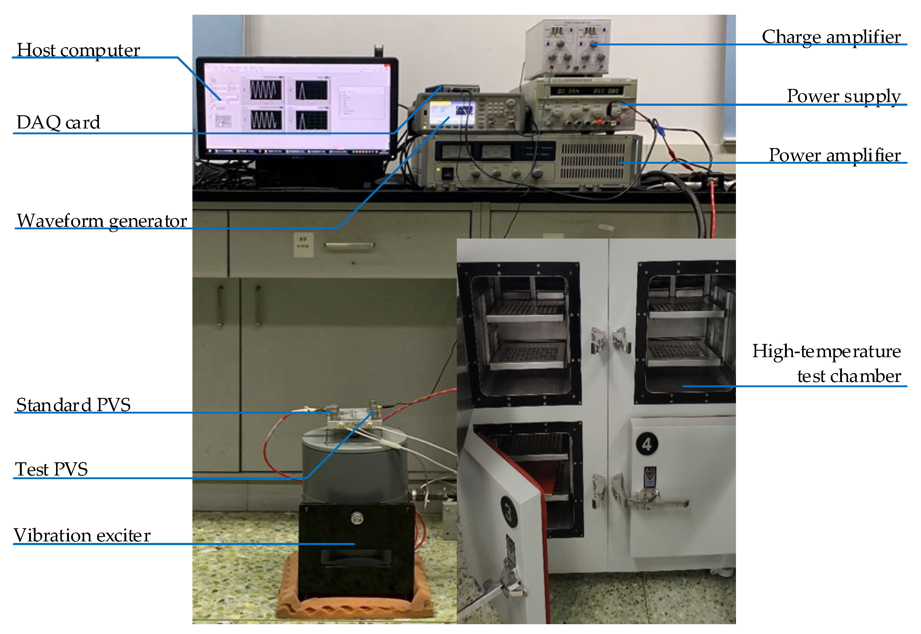
To validate the DT model of a PVS during the task of sensitivity degradation, a verification platform is established. A photograph of the test rig is shown in Figure 9.
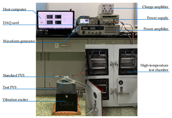
Figure 9.
Experimental platform.
During this test, a test PVS and a standard PVS are embedded in a vibration exciter for sensitivity degradation monitoring. The vibration signals are transformed through a charge amplifier, detected using a data acquisition (DAQ) card, and recorded with a host computer. We use a power supply as the electric source of the experimental system and a waveform generator for system debugging. In addition, a high-temperature test chamber is used to simulate the thermal stress condition. The specifications of each piece of equipment are given in Table 2.
Table 2.
Test equipment specifications.
Eight PVSs are randomly selected from the same batch and divided into four groups, namely, A, B, C, and D, for the sensitivity degradation test, which are labeled as (A1, A2), (B1, B2), (C1, C2), and (D1, D2), respectively. Aiming at revealing the effectiveness of our approach, the individual variation between the two samples in the same group is neglectable. The test procedures for all groups are presented as follows:
- All PVSs are placed in the high-temperature test chamber and heated at a fixed rate;
- The PVSs are removed from the high-temperature test chamber with a fixed cooling rate and embedded on the vibration exciter;
- The acceleration is set at 100 Hz and 10 g, and the test PVSs’ function and sensitivity are set;
- As long as a malfunction or sensitivity degradation reaches 20%, the test is terminated.
Notably, the temperature varies for different PVS groups, as listed in Table 3.
Table 3.
Test temperature.
5.2. Experimental Results
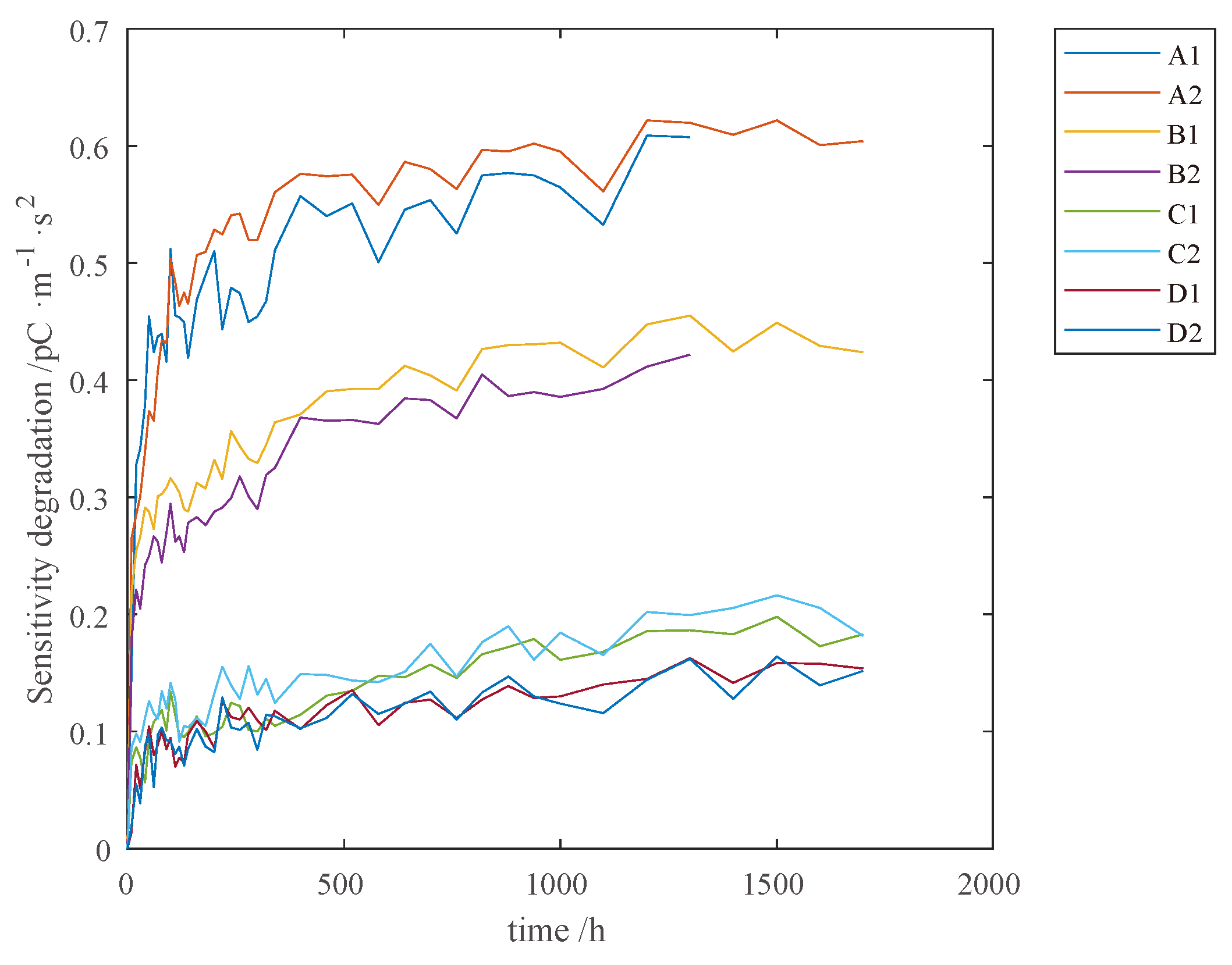
The sensitivity degradation of distinctive PVSs is presented in Figure 10. The X-axis represents the test time, whilst the Y-axis stands for the variation in sensitivity. For each test sample, the degradation of sensitivity is performed in a non-monotonic process. By contrast, the degradation curves for PVSs in the same group are similar to each other due to the identical conditions during the test. One can observe that the higher the temperature, the faster the degradation rate, and thus, a greater degradation amount is accumulated.

Figure 10.
Sensitivity degradation of PVS samples.
5.3. Model Fitting and Verification
5.3.1. Sensitivity Degradation Model Test
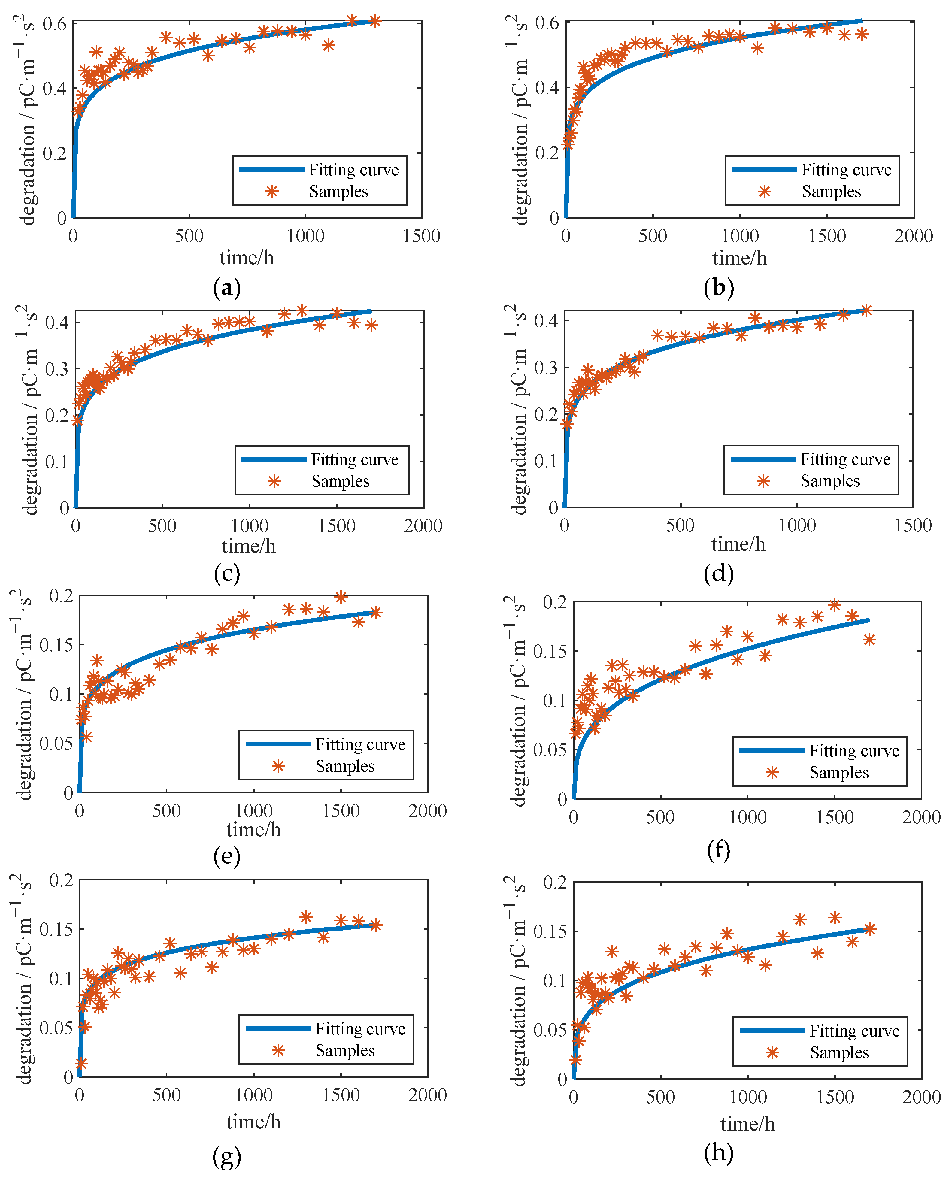
As pointed out in the sensitivity degradation modeling, the degradation process is characterized by three parameters, i.e., , and . In line with the MLE method, the parameter fitting results at four diversified temperatures are listed in Table 4. We also report the sensitivity degradation trajectories in Figure 11.
Table 4.
Sensitivity Degradation Model Parameter Fitting.
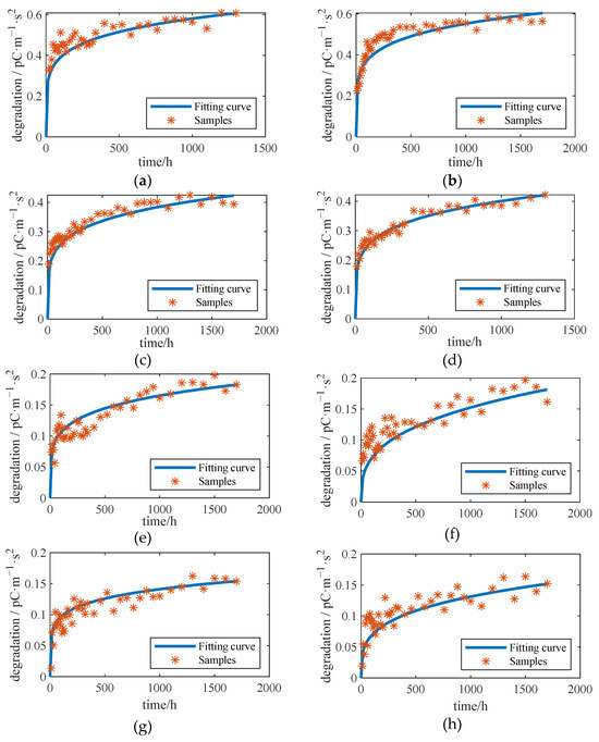
Figure 11.
Sensitivity Degradation Model Fitting Results: (a) sample A1, (b) sample A2, (c) sample B1, (d) sample B2, (e) sample C1, (f) sample C2, (g) sample D1 and (h) sample D2.
For each sample, we have where and . Only if the fitting result is identical to this distribution can the degradation model be recognized as suitable. Accordingly, the hypothesis of is transformed into . Then, the K-S test is applied to investigate the standard normal distribution hypothesis. All the test p-values for the degradation samples exceed 0.05 (Table 5). The hypothesis at this stage is not rejected, confirming the feasibility of the proposed sensitivity degradation model.
Table 5.
Sensitivity degradation model verification based on the K-S test.
Furthermore, the accelerated degradation is described using the parameter set , and , which conforms to:
Given that the degradation process is distinguished for each sample, the estimated values of the degradation parameters are randomly distributed even at the same stress level. The resolution of Equation (36) is transformed into the significance test of with and with , respectively, and then an analysis of variance (ANOVA) is used. If the p-value from the ANOVA is smaller than 0.05, these two items are significantly different, and vice versa. Assuming that the parameters of the two samples fail to satisfy Equation (36), their degradation mechanisms are distinct. In this way, the degradation data under at least one stress condition is unfounded and cannot be applied to parameter estimation in the accelerated degradation model. As shown in Table 6, a temperature of 423.15 K is used for the hypothesis test against the degradation model under other conditions, respectively. The p-values calculated in the ANOVA analysis are reported.
Table 6.
ANOVA-calculated p-values of parameters under different conditions.
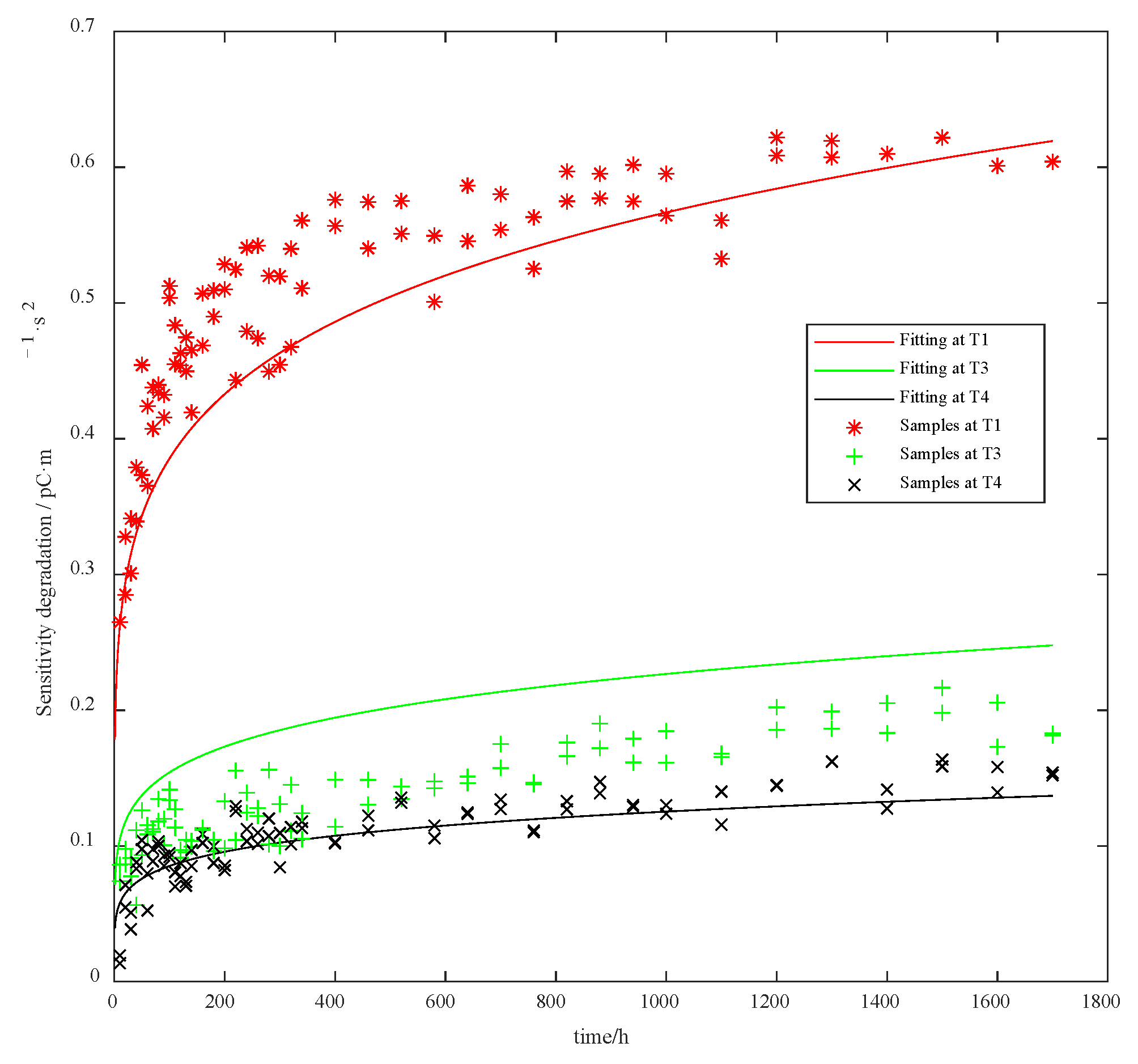
One can observe that the p-value between the parameters T2 and T4 is smaller than 0.04, indicating their degradation mechanisms are distinguished. With respect to the accelerated degradation model, the degradation data for T2 are removed. We thus use the three sets of data for parameter estimation. The Wiener–Arrhenius accelerated degradation model established from the estimated parameters is derived as follows:
with and , and the fitting results are shown in Figure 12.
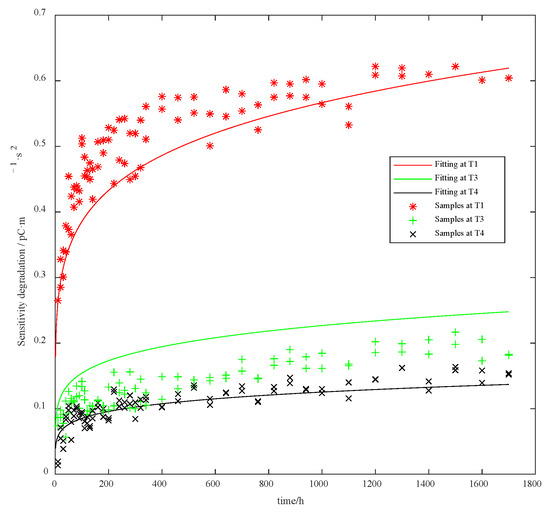
Figure 12.
PVS sensitivity accelerated degradation model fitting results.
According to Figure 12, our model generally covers the distribution of the given samples.
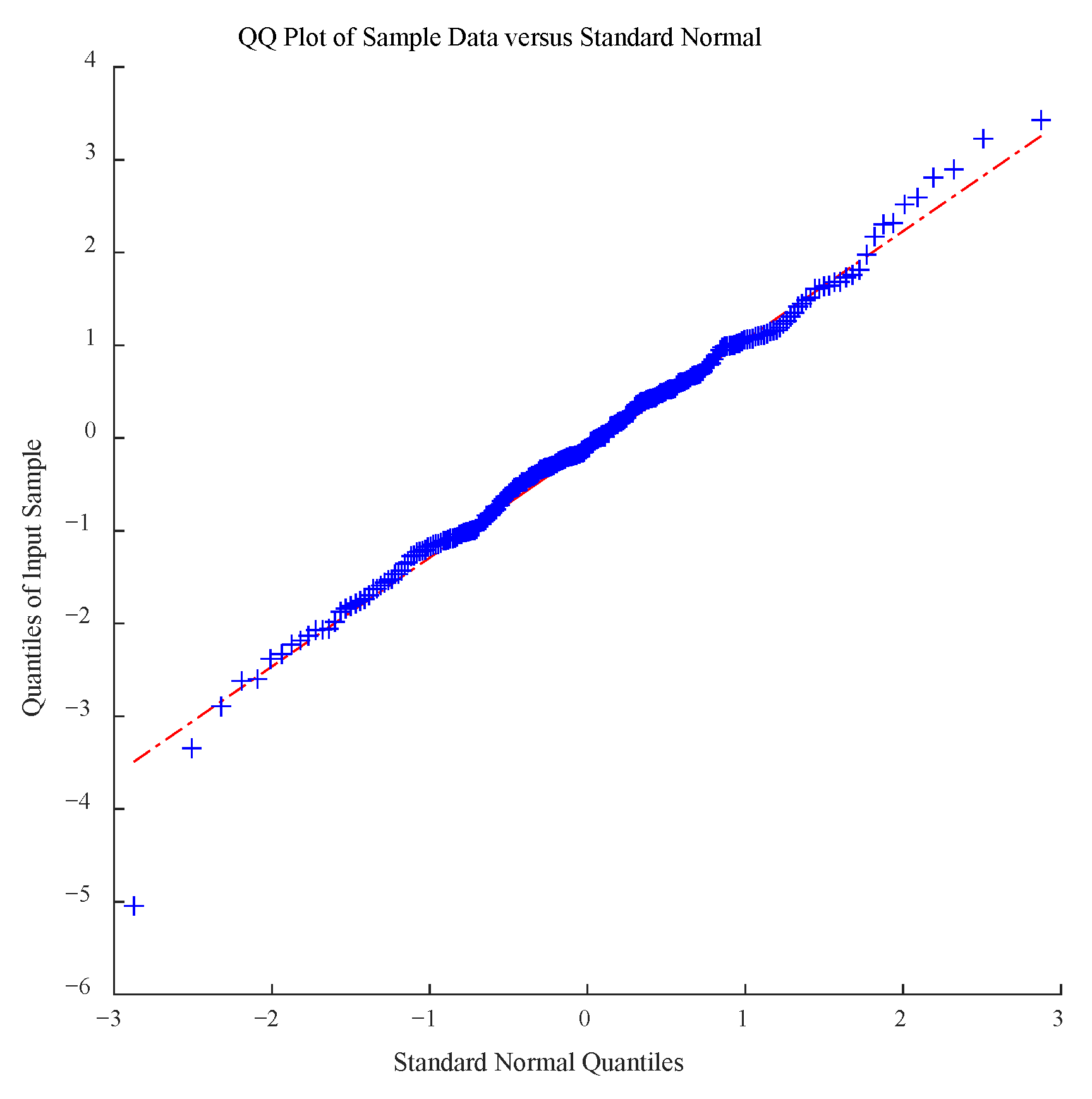
Likewise, for the sample in the accelerated degradation model, we have , which can be transformed into . Subsequently, the K-S test can be applied to verify the standard normal distribution of samples and, thus, the validity of the model.
The p-value of the K-S test is 0.0822, which is greater than 0.05, indicating that the model is suitable for describing accelerated sensitivity degradation. The degradation data tested using QQ-plot are shown in Figure 13.
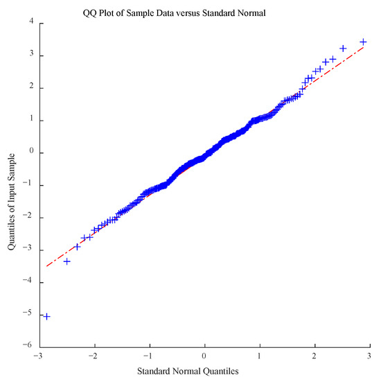
Figure 13.
QQ-plot test results for the standard normal distribution.
5.3.2. Dynamic Error Correction Analysis
The degradation test of sample E from the sample set is conducted at a temperature of 493.15 K. Based on the accelerated degradation model in Equation (40), we have:
As presented in Equation (22), the degradation process of sample E can be modeled to predict the degradation data and the error . Specifically, the first 100 h of data are used for error prediction while the model is corrected at the 100th h. According to Table 7, we obtain the AIC values of the error models in Table 1. The computation of each AIC value is given in Appendix B.
Table 7.
AIC value of four error models.
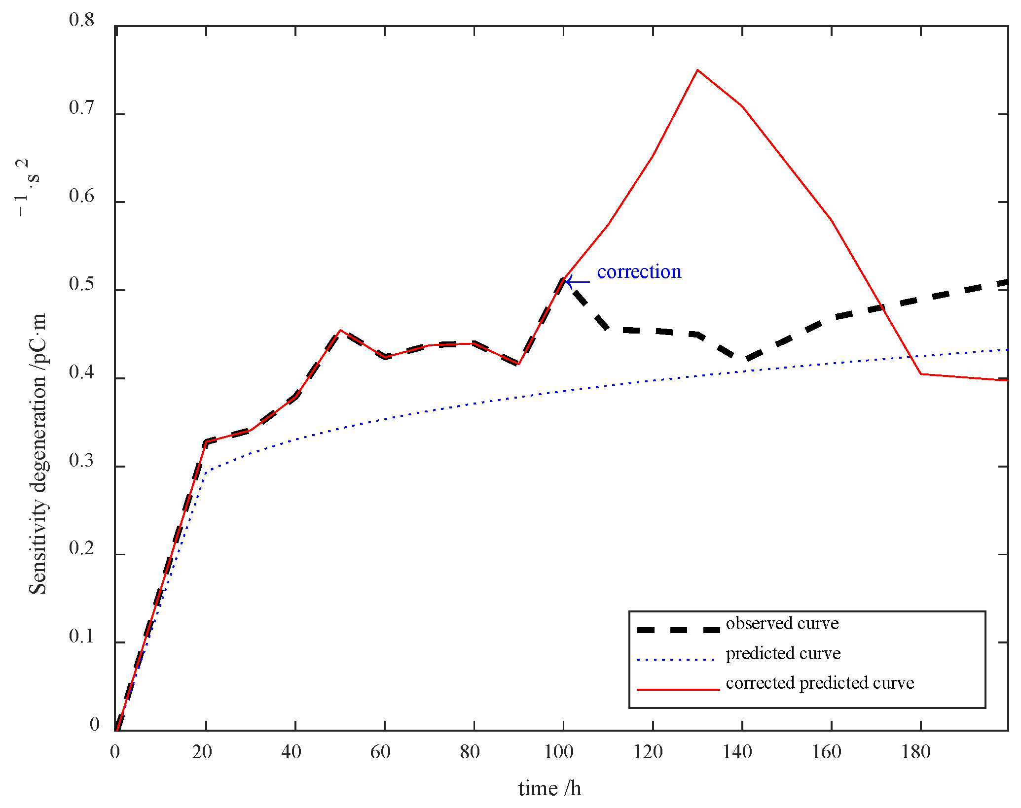
Based on AIC, M4 is selected for error fitting, which is:
where .
The revised sensitivity degradation error prediction is shown in Figure 14, which reveals the effectiveness of the AIC-based error correction scheme.
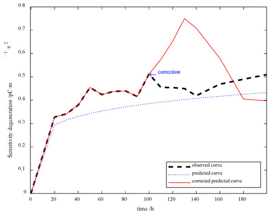
Figure 14.
Revised sensitivity degradation prediction outcomes.
Notwithstanding, the predicted error continues to increase after the first time model correction. For this reason, the 100 to 200 h degradation data are applied to correct the error at the 200th h, and so is that at the 300th h. In this experiment, three time error corrections were carried out, whose results are shown in Figure 15.
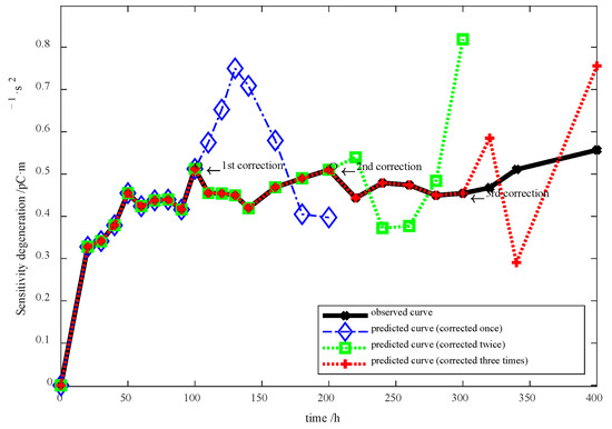
Figure 15.
Sensitivity degradation prediction outcomes with different time error corrections.
5.3.3. RUL Prediction Results
With respect to sample E, we can compute its degradation drift coefficient and diffusion coefficient using Equations (16) and (17) as and . The first 100 h of real-time degradation data are used for error correction. The parameters of the revised sensitivity degradation model are presented in Table 8.
Table 8.
Parameters of the revised sensitivity degradation model.
In line with Equation (35), the revised sensitivity degradation model satisfies:
Let , , , and , . Then, Equation (43) is converted to:
Substituting Equation (44) into Equation (36), we have:
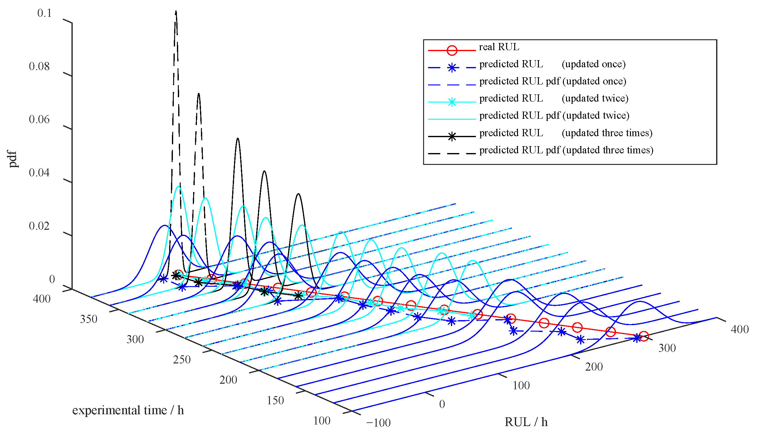
The estimation of remaining life is computed as . The 95% confidence interval for the predicted RUL at the 100th h is (230, 350) h, consistent with the measured 300th h RUL. The probability density function for the predicted RUL is shown in Figure 16. The probability density function narrows over time, indicating that the uncertainty in the RUL prediction results declines. In addition, with the increasing error correction times, an even higher RUL prediction accuracy is achieved. After three time error corrections, the prediction of RUL at the 300th h is 92 h, with a 95% confidence interval of (83, 104) h, which approaches the measured RUL of 100 h. In contrast, the RUL prediction outcome without error correction is 343 h at the 300th h, which has a considerable gap compared with the measured RUL of 100 h. In this way, it is reasonable to expect better-predicting performance of our model, as is the case.
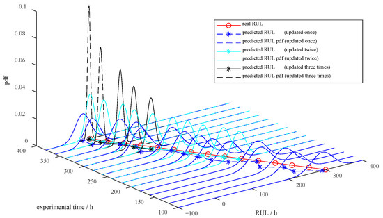
Figure 16.
RUL prediction results with different times of model updates using real-time data.
5.4. Case Study
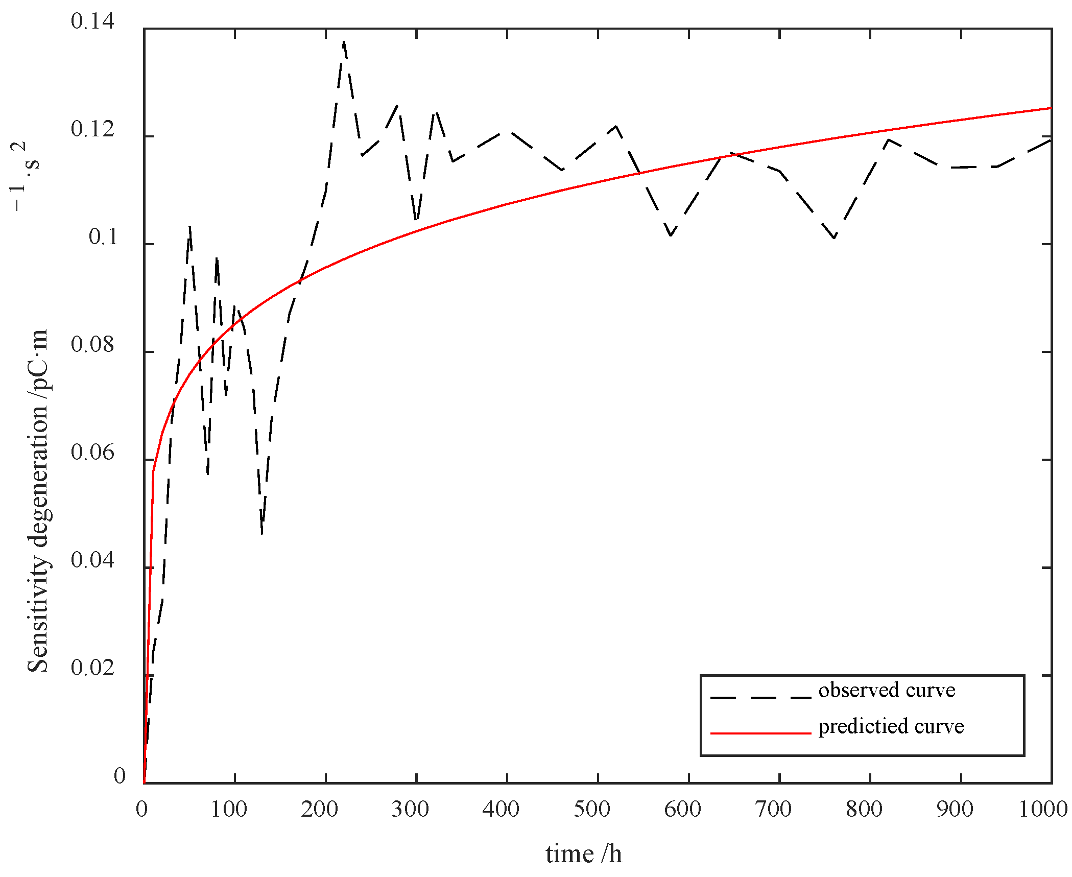
In line with the aforementioned procedures, a DT model of a PVS is established for RUL prediction. A set of PVS samples works at a temperature of 423.15 K, aiming at simulating the accelerated degradation process. Their working parameters can be sent to the DT model. Key parameters are obtained from the historical degradation data in the DT model, as listed in Table 9. A comparison of the predicted result and the observed result is shown in Figure 17.
Table 9.
Sensitivity degradation model parameters.
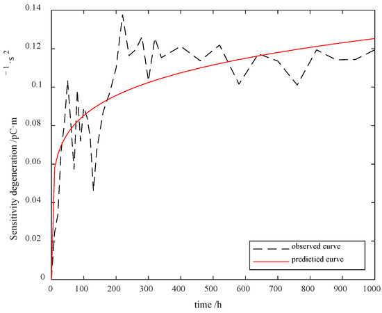
Figure 17.
RUL prediction results compared with the observed results.
The randomness of individual sensitivity degradation challenges precisely describes the degradation process with the basic prediction model. For this reason, the model modification is performed every 200 h by applying the DT real-time data to the sensitivity degradation analysis. The AIC values of the four error models are reported in Table 10.
Table 10.
AIC value of four error models.
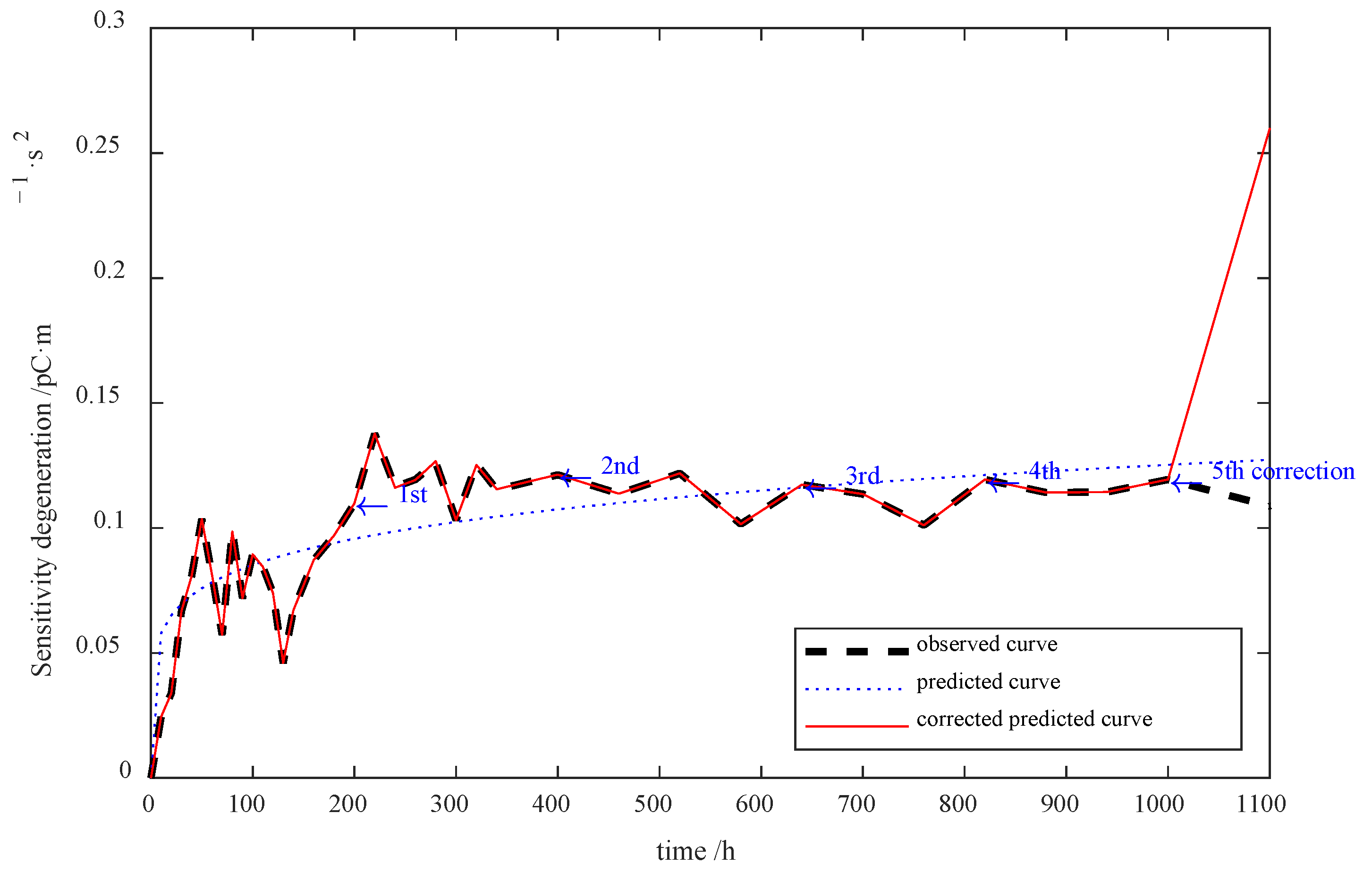
The error model with the smallest AIC is used for error correction each time. Figure 18 shows the revised sensitivity degradation prediction results.
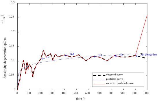
Figure 18.
Sensitivity degradation of sample E.
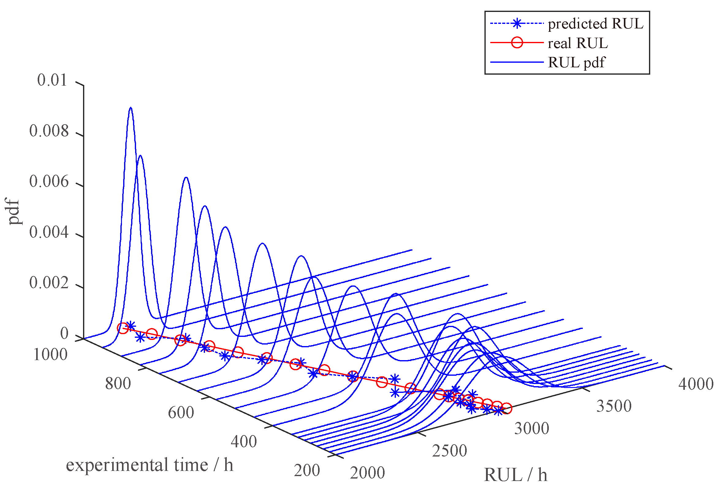
In such a manner, the model is further modified using the real-time data from DT. We obtain the 95% confidence interval for the RUL as (183.4, 214.7) h with the test processing set to 1000 h. The prediction is typically consistent with the observed RUL of 200 h in this experiment. The pdf of the RUL is illustrated in Figure 19. One can observe that the longer the interaction time with DT, the smaller the variance in the RUL prediction. As a result, the RUL prediction accuracy is substantially increased.
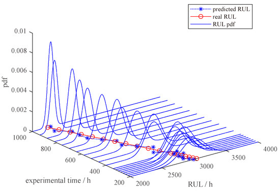
Figure 19.
PVS RUL prediction results for sample E.
5.5. Discussion
In summary, the experimental results show that the proposed DT framework has distinctiveness in sensitivity degradation modeling of working PVS. Sensitivity degradation data are detected and generated in line with the DT framework, which is further applied to characterize the degradation process of a PVS under severe conditions. Moreover, the DT-based RUL prediction algorithm shows its superiority according to the experimental results. A Wiener–Arrhenius accelerated degradation model is built and verified using historical data and then revised. In addition, dynamic error correction and parameter updating are performed based on real-time degradation data. Specifically, the prediction method can effectively identify the RUL of PVS samples with different working hours. With the application of error correction, the prediction accuracy can be further improved in practical use.
Considering the multiple processes from model establishment to RUL prediction, no state-of-the-art methods are available for comparison. However, we compared our approach with the model without error correction. The experimental results for real PVS samples substantially highlight the effectiveness of our RUL prediction algorithm with high accuracy.
6. Conclusions
In this paper, a DT framework for RUL prediction of a PVS is proposed. To start with, on the basis of a five-dimensional model, the establishment of the DT model in five dimensions is analyzed, with a focus on signal modeling, structure simplification, and RUL prediction in VE. Furthermore, six modules, together with their relationship within the DT framework, are depicted. In the scope of RUL prediction, an accelerated degradation model that exploits historical degradation data is built. In addition, methods for error correction and parameter adjustment of the degradation model are put forward. Experiments are carried out on PVS samples to predict the RUL based on real-time degradation data. The experimental results reveal that an accurate RUL prediction result can be achieved in practical use. The following conclusions can be drawn:
- (1)
- The DT framework comprehensively characterizes the structure and working principle of PVSs, precisely performing the sensitivity degradation process. Although onboard degradation data are absent, the operation data can be measured and generated based on the DT model, which is further applied to RUL prediction.
- (2)
- Considering the high-temperature condition, a Wiener–Arrhenius accelerated degradation model is built using historical degradation data from DT. The proposed model is optimized with error correction using the AIC criterion and parameter updating using the Bayesian method, based on which the RUL is thus computed.
- (3)
- Experiments on real PVS samples demonstrate the technical efficacy of our model. A RUL prediction is carried out with the integration of real-time degradation data. Compared with the measured RUL, the prediction result is obtained with a high accuracy.
Author Contributions
Conceptualization, C.G.; methodology, C.F. and C.G.; software, C.F.; validation, C.F. and C.G.; formal analysis, C.G.; investigation, C.F.; resources, C.G.; data curation, C.F.; writing—original draft preparation, C.F.; writing—review and editing, C.G. and W.Z.; visualization, C.F.; supervision, C.G. and W.Z.; project administration, C.G.; funding acquisition, C.G. All authors have read and agreed to the published version of the manuscript.
Funding
This research was funded by the equipment research project in advance Grant No. 41402040301 and research fund NO.2021-0048/YZQT0003.
Institutional Review Board Statement
Not applicable.
Informed Consent Statement
Not applicable.
Data Availability Statement
The data are available from the authors upon request.
Conflicts of Interest
The authors declare no conflict of interest.
Appendix A
Appendix A.1. Structure of a Simplified Shear PVS
In practice, a vibration is delivered from the base to the piezoelectric strip and reaches the mass block, which sets the foundation for further analysis. In this way, these three components are preserved with only the structural details simplified. For model optimization, the modal analysis of a shear-type PVS is carried out by setting a threshold of natural frequency offset less than 1%, as listed in Table A1.
Table A1.
Component simplification of a shear-type PVS.
Table A1.
Component simplification of a shear-type PVS.
| Simplified Components | Natural Frequency/Hz | Deviation/% |
|---|---|---|
| - | 7158.0 | - |
| Insulation strip | 7158.8 | 0.01 |
| Insulation sleeve | 7165.7 | 0.11 |
| Conducting strip | 7219.2 | 0.85 |
| Connector | 7157.1 | −0.01 |
| Cover | 7158.1 | 0.00 |
| Nut | 7034.6 | −1.72 |
| Bolt | 7386.7 | 3.20 |
| Insulation strip, insulation sleeve, conducting strip, connector and cover | 7226.9 | 0.96 |
According to the modal analysis results, components with smaller sizes and masses make minor contributions to the natural frequency, conforming to the mechanics of materials theory. One can observe that five types of components are maintained in a shear-type PVS, which are a base, piezoelectric strips, mass blocks, nuts, and a pre-load screw. The structural details of these components, especially the mounting, connecting, and wiring fixtures, are further analyzed for simplification, as listed in Table A2. With the preservation of the nut assembly fixture, the simplified structure of a shear-type PVS is confirmed.
Table A2.
Assembly details of a simplified a shear-type PVS.
Table A2.
Assembly details of a simplified a shear-type PVS.
| Simplified Structure | Natural Frequency/Hz | Deviation/% |
|---|---|---|
| - | 7158.0 | - |
| Base wiring hole | 7161.6 | 0.05 |
| Connector–base connection | 7154.4 | −0.05 |
| Base mounting hole | 7134.0 | −0.34 |
| Housing–base connection | 7155.9 | −0.03 |
| Nut chamfer and wedge cut | 6982.4 | −2.45 |
| Base wiring hole, connector–base connection, base mounting hole, and housing–base connection | 7128.2 | −0.42 |
Appendix A.2. Structure of a Simplified Compression-type PVS
Likewise, we obtain a simplified structure of compression-type PVS by retaining the base, the piezoelectric strips, the conducting strips, the seismic mass, and the pre-load screw (Table A3) while ablating the assembly details (Table A4).
Table A3.
Component simplification of a compression-type PVS.
Table A3.
Component simplification of a compression-type PVS.
| Simplified Components | Natural Frequency/Hz | Deviation/% |
|---|---|---|
| - | 13,253 | - |
| Connector | 13,236 | −0.13 |
| Housing | 13,252 | −0.01 |
| Insulation strip | 13,253 | 0.00 |
| Conducting strip | 19,542 | 47.45 |
| Connector, housing, and insulation strip | 13,227 | −0.20 |
Table A4.
Assembly details of a simplified compression-type PVS.
Table A4.
Assembly details of a simplified compression-type PVS.
| Simplified Structure | Natural Frequency/Hz | Deviation/% |
|---|---|---|
| - | 13,253 | - |
| Base mounting hole | 13,237 | −0.12 |
| Connector–base connection | 13,236 | −0.13 |
| Screw mounting hole | 13,236 | −0.13 |
| Bottom mounting hole, connector–base connection, and screw mounting hole | 13,237 | −0.12 |
Appendix B
Appendix B.1. Error Model 1
For with , we have . The log-likelihood function is established as:
The values of , and are computed using MLE. The outcome of is derived from Equation (24).
Appendix B.2. Error Model 2
For with , we have . The log-likelihood function is established as:
The values of , and are computed using MLE. The outcome of is derived from Equation (24).
Appendix B.3. Error Model 3
For with , we have . The log-likelihood function is established as:
The values of , and , , …, are computed using MLE at different positive integers . The outcomes of the with different are derived from Equation (24), the maximum of which is taken as .
Appendix B.4. Error Model 4
For with , we have . The log-likelihood function is established as:
The values of , , , , …, , , , …, and , , …, are computed using MLE at different positive integers . The outcomes of the with different are derived from Equation (24), the maximum of which is taken as .
References
- Xia, C.J.; Zhan, Y.Y.; Tan, Y.; Wu, W.Q. Research on Forecasting Aeroengine Vibration Signals Based on the MAE Model. IEEE Access 2022, 10, 110676–110688. [Google Scholar] [CrossRef]
- Xiong, M.L.; Wang, H.W.; Fu, Q.; Xu, Y. Digital twin-driven aero-engine intelligent predictive maintenance. Int. J. Adv. Manuf. Technol. 2021, 114, 3751–3761. [Google Scholar] [CrossRef]
- Zhang, C.Q.; Cui, L.F.; Zhang, Q.Z.; Jin, Y.; Han, X.X.; Shi, Y. Online Anomaly Detection for Aeroengine Gas Path Based on Piecewise Linear Representation and Support Vector Data Description. IEEE Sens. J. 2022, 22, 22808–22816. [Google Scholar] [CrossRef]
- Yu, F.P.; Hou, S.; Zhao, X.; Zhang, S.J. High-Temperature Piezoelectric Crystals ReCa4O(BO3)(3): A Review. IEEE Trans. Ultrason. Ferroelectr. Freq. Control 2014, 61, 1344–1356. [Google Scholar] [CrossRef]
- How Vibration Informs the Maintenance of Aircraft Engines. Available online: https://www.aerospacetestinginternational.com/features/how-vibration-data-informs-the-maintenance-of-aircraft-engines.html (accessed on 8 January 2023).
- Trivedi, S.; Ganesh, R.H.; Shen, T.; Huang, P.W.; Li, S.S. Piezoelectric MEMS Vibration Sensor Module for Machining Quality Prediction. In Proceedings of the IEEE Sensors Conference, Virtual, 25–28 October 2020; Electr Network. IEEE: Piscataway, NJ, USA, 2020. [Google Scholar]
- Yuan, Y.; Liu, X.F.; Ding, S.T.; Pan, B.C. Fault Detection and Location System for Diagnosis of Multiple Faults in Aeroengines. IEEE Access 2017, 5, 17671–17677. [Google Scholar] [CrossRef]
- Jiang, C.; Liu, X.L.; Yu, F.P.; Zhang, S.J.; Fang, H.R.; Cheng, X.F.; Zhao, X. High-temperature Vibration Sensor Based on Ba2TiSi2O8 Piezoelectric Crystal With Ultra-Stable Sensing Performance up to 650 degrees C. IEEE Trans. Ind. Electron. 2021, 68, 12850–12859. [Google Scholar] [CrossRef]
- Wei, H.F.; Geng, W.P.; Bi, K.X.; Li, T.; Li, X.M.; Qiao, X.J.; Shi, Y.K.; Zhang, H.Y.; Zhao, C.Q.; Xue, G.; et al. High-Performance Piezoelectric-Type MEMS Vibration Sensor Based on LiNbO3 Single-Crystal Cantilever Beams. Micromachines 2022, 13, 329. [Google Scholar] [CrossRef]
- Liu, Y.; Sun, B. Remaining Useful Life Prediction of MEMS Sensors Used in Automotive Under Random Vibration Loading. In Proceedings of the 59th Annual Reliability and Maintainability Symposium (RAMS), Orlando, FL, USA, 28–31 January 2013; IEEE: Orlando, FL, USA, 2013. [Google Scholar]
- Jiang, C.; Jiang, R.H.; He, W.; He, J.N. Comparative Experiments of Optical Fiber Sensor and Piezoelectric Sensor based on Vibration Detection. In Proceedings of the 4th IEEE International Conference on Frontiers of Sensors Technologies (ICFST), Electr Network, Shanghai, China, 6–9 November 2020; IEEE: Piscataway, NJ, USA, 2020; pp. 17–20. [Google Scholar]
- Rainer, S.; Thomas, D. Digital Twin. In CIRP Encyclopedia of Production Engineering, 1st ed.; Springer: Heidelberg, Berlin, 2019. [Google Scholar]
- Hartmann, D.; Van der Auweraer, H. Digital Twins. In Progress in Industrial Mathematics: Success Stories, 9th ed., Proceedings of the International Congress on Industrial and Applied Mathematics (ICIAM), Univ Valencia, Valencia, Spain, 15–19 July 2019; Springer International Publishing Ag: Univ Valencia: Valencia, Spain, 2019; pp. 3–17. [Google Scholar]
- Feng, K.; Ji, J.C.; Zhang, Y.C.; Ni, Q.; Liu, Z.; Beer, M. Digital twin-driven intelligent assessment of gear surface degradation. Mech. Syst. Signal Proc. 2023, 186, 109896. [Google Scholar] [CrossRef]
- Khadim, Q.; Hagh, Y.S.; Pyrhonen, L.; Jaiswal, S.; Zhidchenko, V.; Kurvinen, E.; Sopanen, J.; Mikkola, A.; Handroos, H. State Estimation in a Hydraulically Actuated Log Crane Using Unscented Kalman Filter. IEEE Access 2022, 10, 62863–62878. [Google Scholar] [CrossRef]
- Jafari, S.; Byun, Y.C. Prediction of the Battery State Using the Digital Twin Framework Based on the Battery Management System. IEEE Access 2022, 10, 124685–124696. [Google Scholar] [CrossRef]
- Don, M.G.; Rideout, G. A Digital Twinning Methodology for Vibration Prediction and Fatigue Life Prognosis of Vertical Oil Well Drillstrings. IEEE Access 2023, 11, 62892–62905. [Google Scholar] [CrossRef]
- Zhuang, C.B.; Liu, J.H.; Xiong, H. Digital twin-based smart production management and control framework for the complex product assembly shop-floor. Int. J. Adv. Manuf. Technol. 2018, 96, 1149–1163. [Google Scholar] [CrossRef]
- Kon, S.; Horowitz, R. A High-Resolution MEMS Piezoelectric Strain Sensor for Structural Vibration Detection. IEEE Sens. J. 2008, 8, 2027–2035. [Google Scholar] [CrossRef]
- Joseph, J.; Ma, B.; Khuri-Yakub, B.T. Applications of Capacitive Micromachined Ultrasonic Transducers: A Comprehensive Review. IEEE Trans. Ultrason. Ferroelectr. Freq. Control 2022, 69, 456–467. [Google Scholar] [CrossRef] [PubMed]
- Ahmad, N.; Ghazilla, R.A.R.; Khairi, N.M.; Kasi, V.J.I.C. Reviews on Various Inertial Measurement Unit (IMU). Sens. Appl. 2013, 1, 256–262. [Google Scholar]
- Roy, K.; Lee, J.E.Y.; Lee, C. Thin-film PMUTs: A review of over 40 years of research. Microsyst. Nanoeng. 2023, 9, 17. [Google Scholar] [CrossRef] [PubMed]
- Tao, F.; Zhang, M.; Liu, Y.S.; Nee, A.Y.C. Digital twin driven prognostics and health management for complex equipment. CIRP Ann.-Manuf. Technol. 2018, 67, 169–172. [Google Scholar] [CrossRef]
- Tao, F.; Liu, W.; Zhang, M.; Hu, T.; Qi, Q.; Zhang, H.; Sui, F.; Wang, T. Five-dimension digital twin model and its ten applications. Comput. Integr. Manuf. Syst. 2019, 25, 1–18. [Google Scholar]
- Wu, C.L.; Chen, T.; Li, Z.B.; Liu, W. A function-oriented optimising approach for smart product service systems at the conceptual design stage: A perspective from the digital twin framework. J. Clean Prod. 2021, 297, 126597. [Google Scholar] [CrossRef]
- Si, X.S.; Wang, W.B.; Hu, C.H.; Zhou, D.H. Remaining useful life estimation—A review on the statistical data driven approaches. Eur. J. Oper. Res. 2011, 213, 1–14. [Google Scholar] [CrossRef]
- Guida, M.; Pulcini, G. The inverse Gamma process: A family of continuous stochastic models for describing state-dependent deterioration phenomena. Reliab. Eng. Syst. Saf. 2013, 120, 72–79. [Google Scholar] [CrossRef]
- Wang, H.W.; Kang, R. Modeling of degradation data via wiener stochastic process based on acceleration factor constant principle. Appl. Math. Model. 2020, 84, 19–35. [Google Scholar] [CrossRef]
- Yang, J.; Zhou, Y.T.; Ma, H.L.; Ding, S.H.; Li, X. The fracture behavior of two asymmetrical limited permeable cracks emanating from an elliptical hole in one-dimensional hexagonal quasicrystals with piezoelectric effect. Int. J. Solids Struct. 2017, 108, 175–185. [Google Scholar] [CrossRef]
- Wang, Y.J.; Gao, C.F.; Song, H.P. The anti-plane solution for the edge cracks originating from an arbitrary hole in a piezoelectric material. Mech. Res. Commun. 2015, 65, 17–23. [Google Scholar] [CrossRef]
- Wang, Z.B.; Zhou, W.Y.; Xiao, Z.J.; Yao, Q.R.; Xia, X.G.; Mei, J.; Zhang, D.; Chen, P.H.; Li, S.Q.; Wang, Y.C.; et al. A High-Temperature Accelerometer with Excellent Performance Based on the Improved Graphene Aerogel. ACS Appl. Mater. Interfaces 2023, 15, 19337–19348. [Google Scholar] [CrossRef]
- Kittaneh, O. On the Theory of the Arrhenius-Normal Model with Applications to the Life Distribution of Lithium-Ion Batteries. Batteries 2023, 9, 55. [Google Scholar] [CrossRef]
- Kong, J.Z.; Wang, D.; Yan, T.T.; Zhu, J.Z.; Zhang, X. Accelerated Stress Factors Based Nonlinear Wiener Process Model for Lithium-Ion Battery Prognostics. IEEE Trans. Ind. Electron. 2022, 69, 11665–11674. [Google Scholar] [CrossRef]
- Ren, C.; Li, H.; Li, T.; Zhang, J.; Si, X. Remaining Useful Life Prediction Method for Equipment with Dynamic Calibration of Degradation Model. Acta Aeronaut. Astronaut. Sin. 2023. preprint. [Google Scholar] [CrossRef]
- Hu, Y.; Wangz, S.; Huang, J.; Takyi-Aninakwa, P.; Chen, X. A Novel Seasonal Autoregressive Integrated Moving Average Method for the Accurate Lithium-ion Battery Residual Life Prediction. Int. J. Electrochem. Sci. 2022, 17, 220555. [Google Scholar] [CrossRef]
- Nguyen, K.T.P.; Fouladirad, M.; Grall, A. Model selection for degradation modeling and prognosis with health monitoring data. Reliab. Eng. Syst. Saf. 2018, 169, 105–116. [Google Scholar] [CrossRef]
- Yu, Y.; Si, X.S.; Hu, C.H.; Zheng, J.F.; Zhang, J.X. Online remaining-useful-life estimation with a Bayesian-updated expectation-conditional-maximization algorithm and a modified Bayesian-model-averaging method. Sci. China Inf. Sci. 2021, 64, 112205. [Google Scholar] [CrossRef]
- Hong, P.; Si, X.S.; Hu, C.H.; Zhang, J.X.; Du, D.B.; Pang, Z.N.; Zhang, S.F. Prognostics based on the generalized diffusion process with parameters updated by a sequential Bayesian method. Sci. China Inf. Sci. 2022, 65, 17. [Google Scholar]
- Wang, Z.Q.; Hu, C.H.; Wang, W.B.; Si, X.S. An Additive Wiener Process-Based Prognostic Model for Hybrid Deteriorating Systems. IEEE Trans. Reliab. 2014, 63, 208–222. [Google Scholar] [CrossRef]
- Hu, C.H.; Pei, H.; Si, X.S.; Du, D.B.; Pang, Z.N.; Wang, X. A Prognostic Model Based on DBN and Diffusion Process for Degrading Bearing. IEEE Trans. Ind. Electron. 2020, 67, 8767–8777. [Google Scholar] [CrossRef]


Disclaimer/Publisher’s Note: The statements, opinions and data contained in all publications are solely those of the individual author(s) and contributor(s) and not of MDPI and/or the editor(s). MDPI and/or the editor(s) disclaim responsibility for any injury to people or property resulting from any ideas, methods, instructions or products referred to in the content. |
© 2023 by the authors. Licensee MDPI, Basel, Switzerland. This article is an open access article distributed under the terms and conditions of the Creative Commons Attribution (CC BY) license (https://creativecommons.org/licenses/by/4.0/).