
An Enhanced RIME Optimizer with Horizontal and Vertical Crossover for Discriminating Microseismic and Blasting Signals in Deep Mines

 ,
, 

 and
and 
Abstract
:1. Introduction
- Through examining and analyzing the RIME algorithm, this paper proposes a novel method called CCRIME, which is based on vertical and horizontal crossover. The introduction of CCRIME not only enhances the quality of the solutions found but also improves the overall search capabilities.
- To enhance the classification capabilities of the FKNN model, a binary version of CCRIME was created through the use of the binary transformation method. This approach aimed to optimize the important parameters inside the FKNN model. The CCRIME-FKNN model, which is optimized for CCRIME, is an abbreviation for the CCRIME-optimized FKNN model.
- The performance of CCRIME, an optimization method based on swarm intelligence, was evaluated using 30 benchmark functions from IEEE CEC2017. The results of this study demonstrated that CCRIME exhibits exceptional performance across several perspectives, establishing it as a highly effective algorithm.
- This study utilized microseismic and blasting images to extract and select appropriate features. Through the application of CCRIME-FKNN, the identification of microseismic and blasting events was successfully achieved, resulting in a high level of accuracy.
2. Related Work
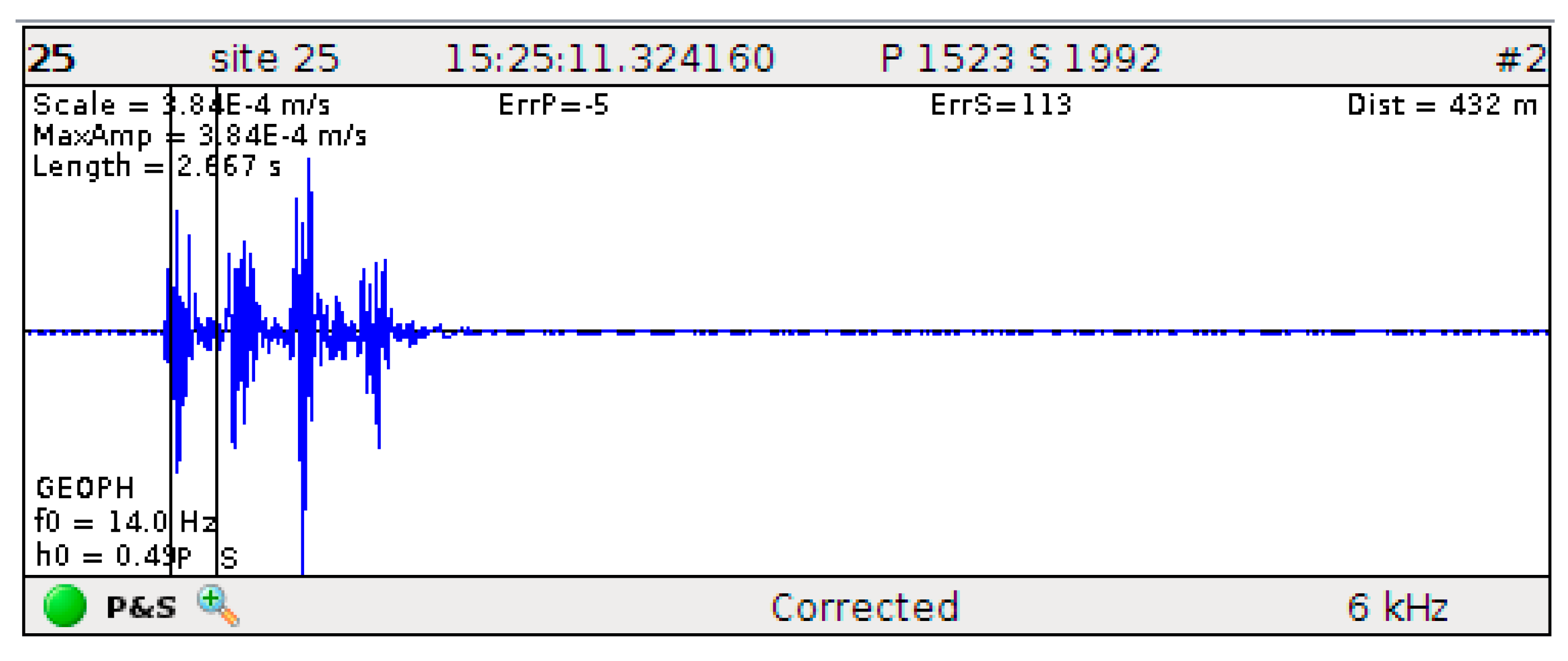
2.1. Data Description
2.2. Microseismicity and Blasting
3. The Proposed CCRIME
3.1. An Overview of RIME
3.2. Horizontal and Vertical Crossover Search
3.3. The Proposed CCRIME
| Algorithm 1 Pseudocode of CCRIME |
| Initialize the population of rime |
| Calculate the fitness of each agent |
| Select the optimal agent |
| While < |
| Update the particle capture probability |
| If |
| Update rime agent location by Equation (10) |
| End If |
| If |
| Cross-updating between agents by Equation (14) |
| End If |
| If |
| Replace with |
| If |
| Replace with |
| End If |
| End If |
| Perform horizontal crossover search and vertical crossover search |
| End While |
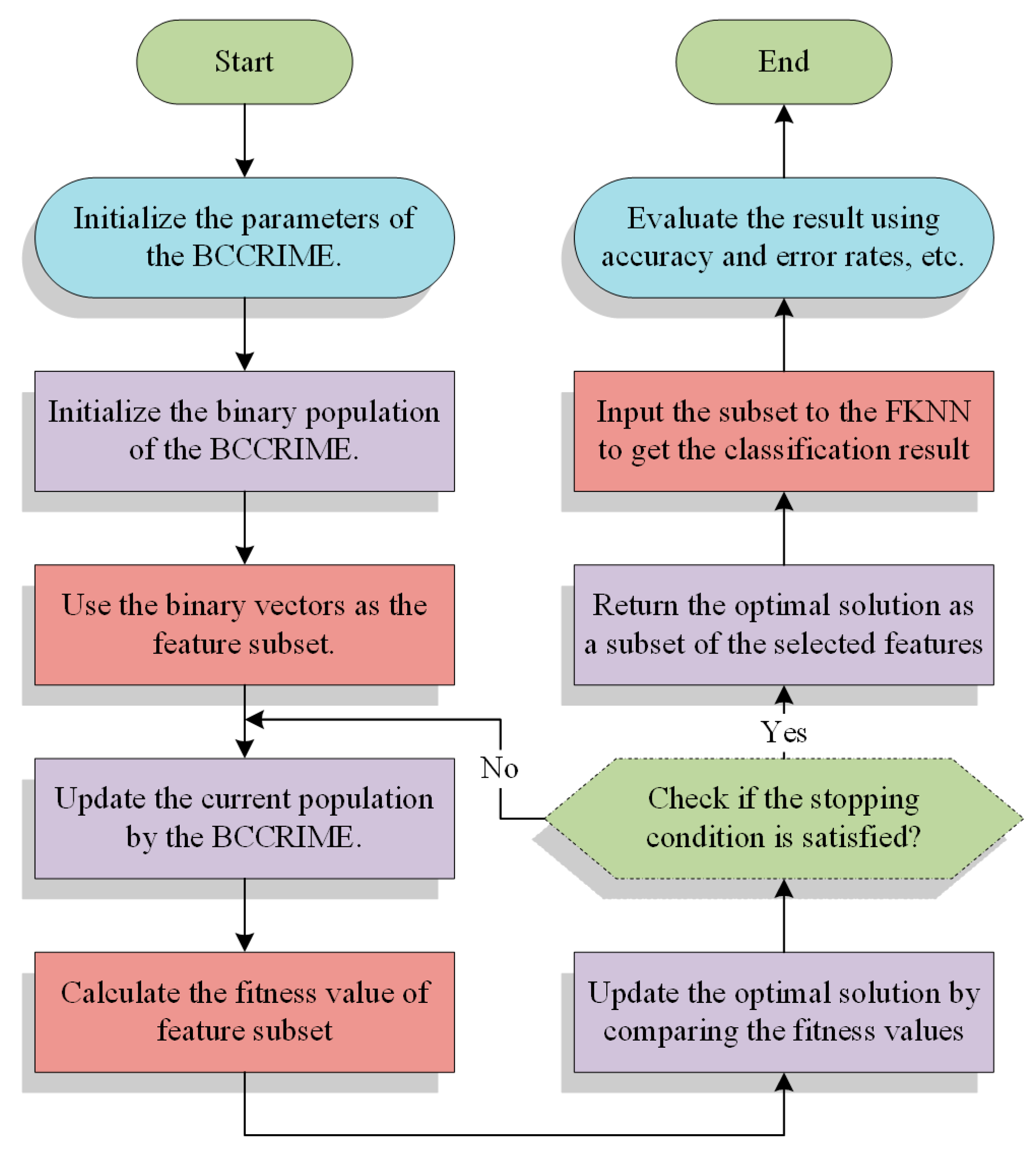
4. The Proposed CCRIME-FKNN Model
4.1. Binary Transformation Method
4.2. Feature Extraction Method
4.3. Fuzzy k-Nearest Neighbor
4.4. The Proposed CCRIME-FKNN Model
5. Experiments, Results, and Analysis
5.1. Benchmark Function Validation
5.1.1. Experimental Setup
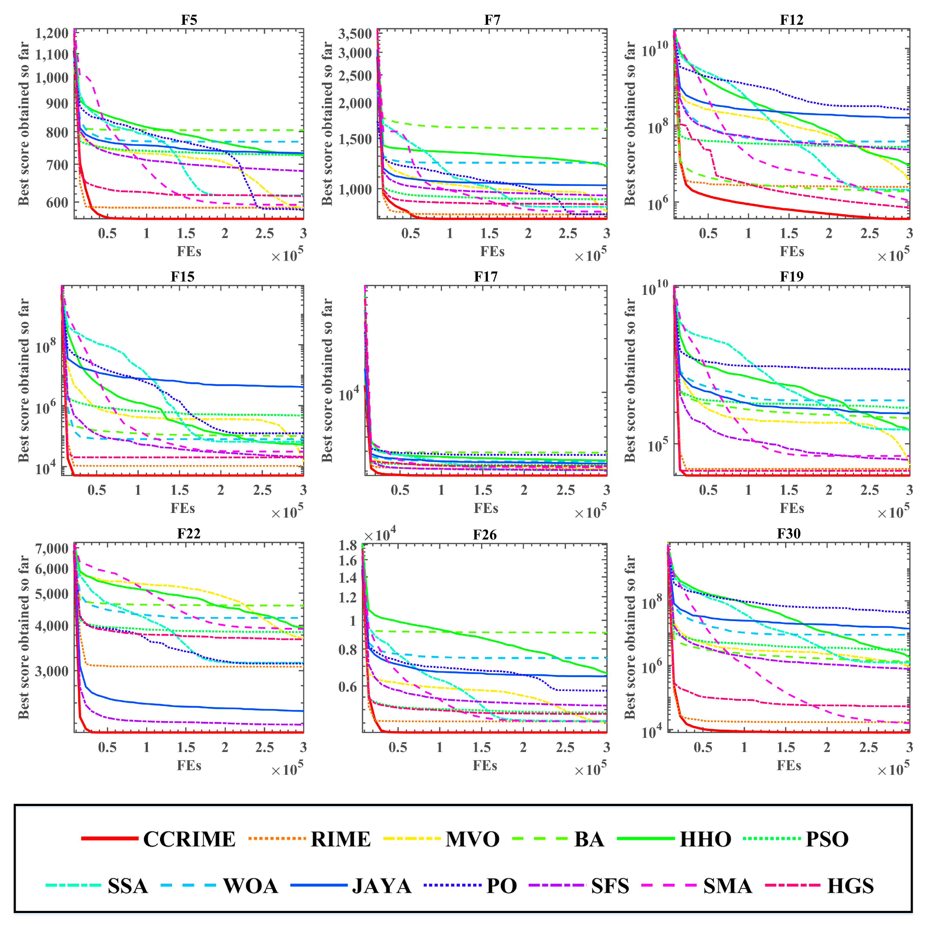
5.1.2. Comparison with Basic Algorithms
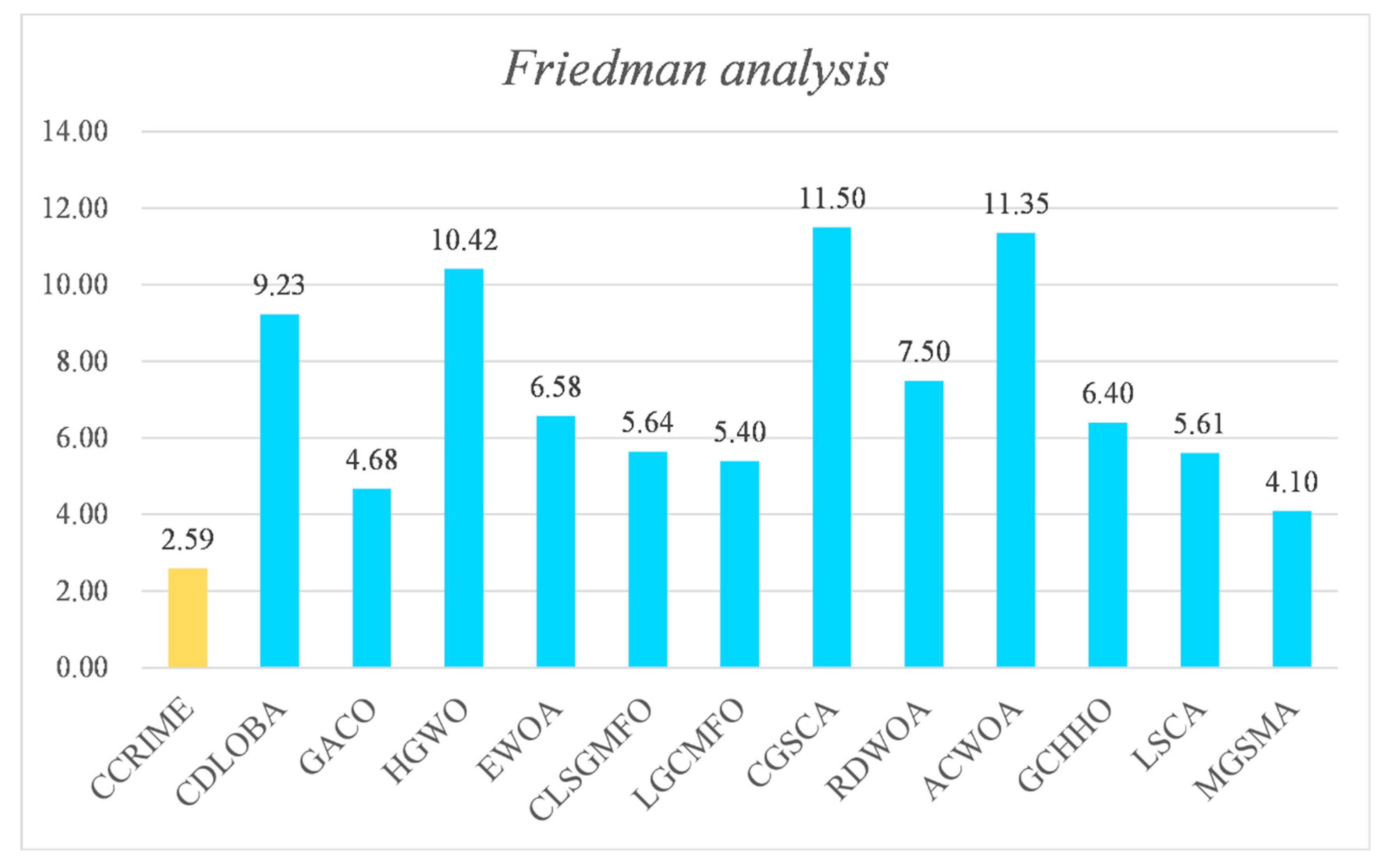
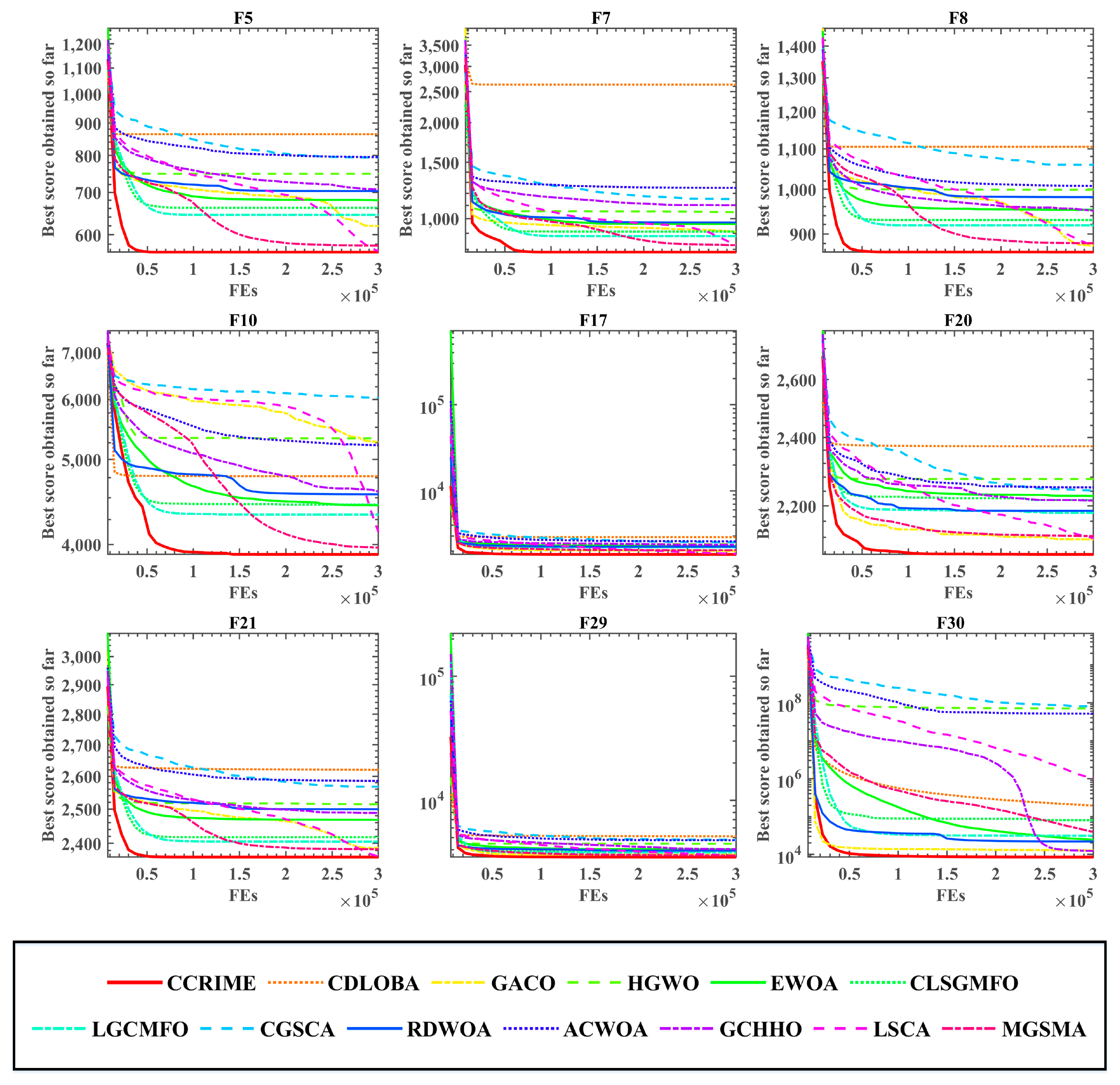
5.1.3. Comparison with State-of-the-Art Variants
5.2. Feature Selection Experiments
5.2.1. Experimental Setup
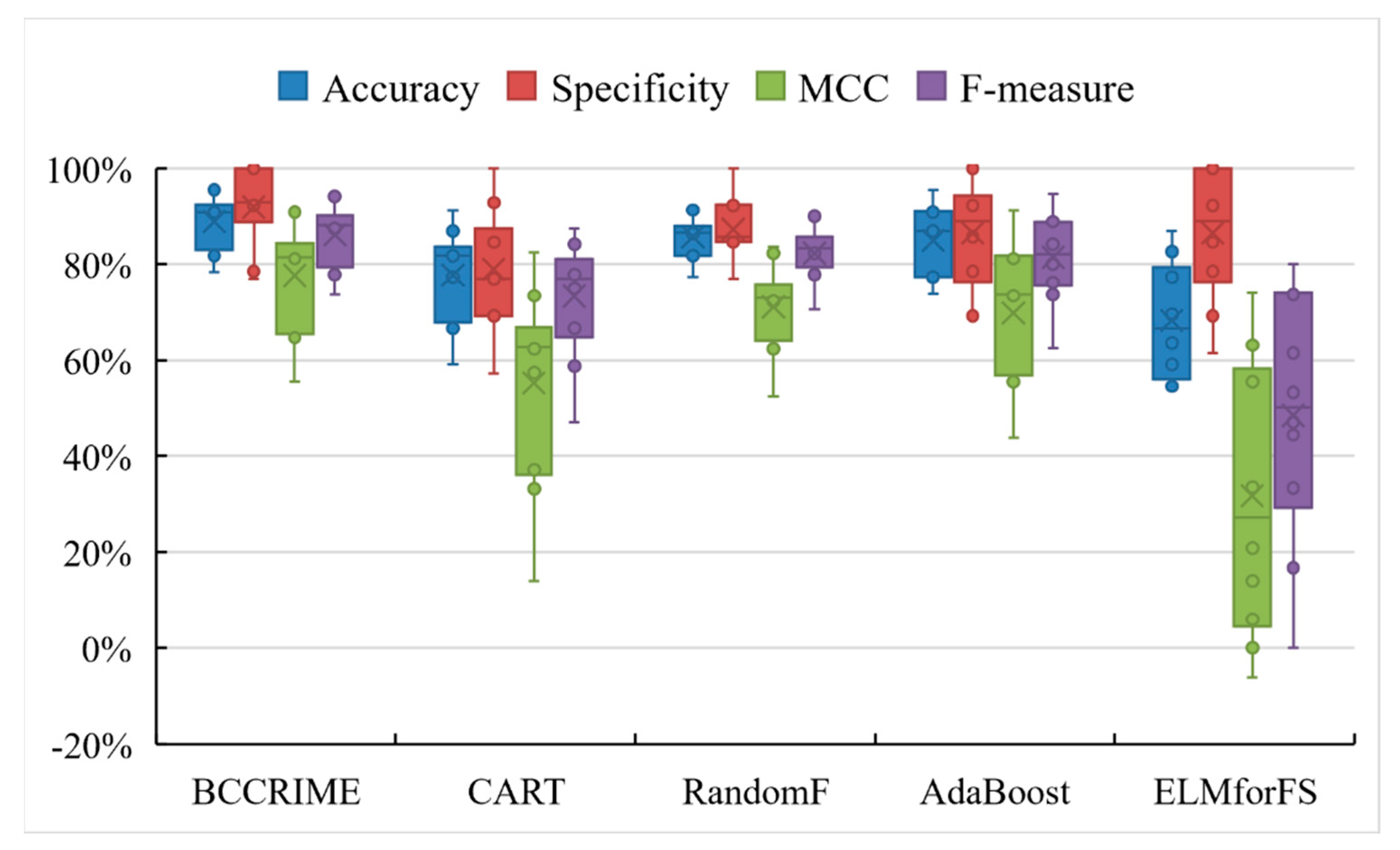
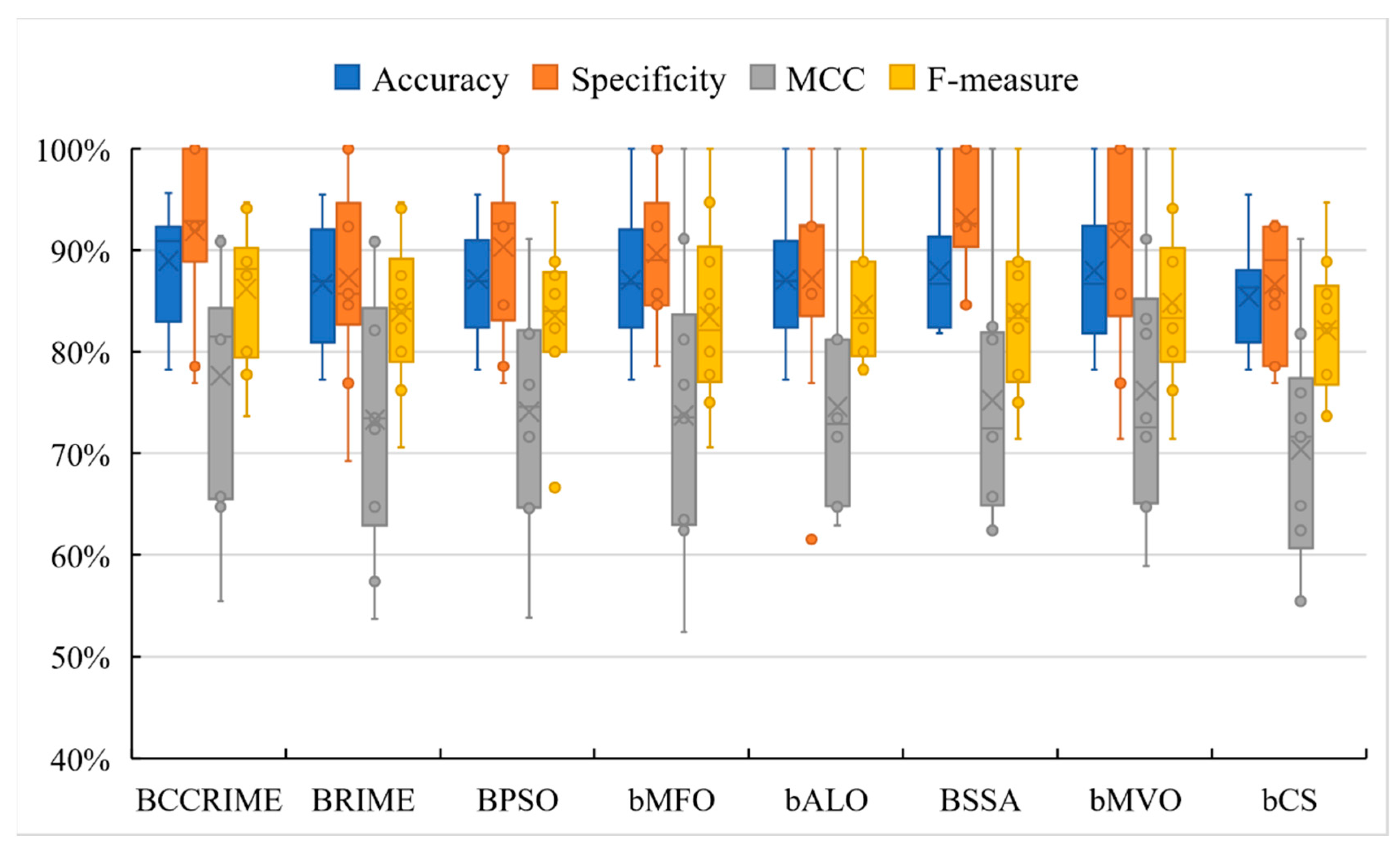
5.2.2. Microseismic and Blast Dataset Experiment
6. Conclusions and Future Directions
Author Contributions
Funding
Data Availability Statement
Acknowledgments
Conflicts of Interest
Appendix A

| F1 | F2 | F3 | ||||
| AVG | STD | AVG | STD | AVG | STD | |
| CCRIME | 4.2352 × 10³ | 4.7608 × 10³ | 2.1640 × 10² | 3.5195 × 101 | 3.0911 × 10² | 5.3019 × 100 |
| RIME | 8.9768 × 10³ | 5.8909 × 10³ | 1.1918 × 10³ | 1.6094 × 10³ | 3.0186 × 10² | 9.5716 × 10⁻¹ |
| MVO | 1.2080 × 10⁴ | 6.8991 × 10³ | 9.2436 × 10² | 1.2608 × 10³ | 3.0037 × 10² | 1.5597 × 10⁻¹ |
| BA | 5.3849 × 10⁵ | 3.6639 × 10⁵ | 2.0000 × 10² | 1.3410 × 10⁻⁴ | 3.0009 × 10² | 8.3596 × 10⁻² |
| HHO | 1.0454 × 10⁷ | 2.0591 × 10⁶ | 6.3435 × 10¹¹ | 1.0304 × 10¹² | 4.9178 × 10³ | 1.8832 × 10³ |
| PSO | 1.3465 × 10⁸ | 1.7454 × 10⁷ | 4.2792 × 10¹³ | 4.5075 × 10¹³ | 6.4025 × 10² | 5.2610 × 101 |
| SSA | 3.9871 × 10³ | 4.9271 × 10³ | 2.0535 × 10² | 1.8872 × 101 | 3.0000 × 10² | 1.0612 × 10⁻⁸ |
| WOA | 3.3518 × 10⁶ | 2.2122 × 10⁶ | 6.8389 × 10²¹ | 2.8707 × 10²² | 1.6825 × 10⁵ | 5.5436 × 10⁴ |
| JAYA | 5.4373 × 10⁹ | 1.0080 × 10⁹ | 2.7325 × 1031 | 1.2670 × 1032 | 4.2467 × 10⁴ | 8.1926 × 10³ |
| PO | 3.7297 × 10⁷ | 8.5935 × 10⁷ | 2.2738 × 1038 | 1.0759 × 1039 | 5.1376 × 10⁴ | 1.1204 × 10⁴ |
| SFS | 2.4036 × 10⁸ | 2.9173 × 10⁸ | 1.1897 × 1024 | 6.4968 × 1024 | 2.5396 × 10⁴ | 7.9311 × 10³ |
| SMA | 7.7115 × 10³ | 7.9786 × 10³ | 2.0000 × 10² | 4.5202 × 10⁻³ | 3.0002 × 10² | 1.7494 × 10⁻² |
| HGS | 5.9547 × 10³ | 3.7800 × 10³ | 2.4649 × 10² | 1.1641 × 101 | 1.5381 × 10³ | 3.5435 × 10³ |
| F4 | F5 | F6 | ||||
| AVG | STD | AVG | STD | AVG | STD | |
| CCRIME | 4.8159 × 10² | 2.2211 × 101 | 5.6016 × 10² | 1.5706 × 101 | 6.0000 × 10² | 4.5903 × 10⁻⁷ |
| RIME | 4.9089 × 10² | 2.3365 × 101 | 5.8617 × 10² | 2.0042 × 101 | 6.0031 × 10² | 2.3598 × 10⁻¹ |
| MVO | 4.8857 × 10² | 3.6765 × 100 | 5.8572 × 10² | 2.8558 × 101 | 6.0790 × 10² | 6.4185 × 100 |
| BA | 4.7796 × 10² | 3.2553 × 101 | 8.0505 × 10² | 4.8012 × 101 | 6.7252 × 10² | 8.1846 × 100 |
| HHO | 5.2696 × 10² | 3.7392 × 101 | 7.2639 × 10² | 3.9574 × 101 | 6.6215 × 10² | 5.2602 × 100 |
| PSO | 4.7087 × 10² | 2.9010 × 101 | 7.2702 × 10² | 3.5931 × 101 | 6.5308 × 10² | 1.5342 × 101 |
| SSA | 4.8848 × 10² | 2.3276 × 101 | 6.1671 × 10² | 3.6354 × 101 | 6.2735 × 10² | 7.2336 × 100 |
| WOA | 5.5205 × 10² | 3.8969 × 101 | 7.6790 × 10² | 5.3069 × 101 | 6.6996 × 10² | 8.9938 × 100 |
| JAYA | 7.6986 × 10² | 5.6320 × 101 | 7.3242 × 10² | 1.4973 × 101 | 6.2064 × 10² | 2.0354 × 100 |
| PO | 5.1868 × 10² | 1.5551 × 10² | 5.8202 × 10² | 5.0596 × 101 | 6.1731 × 10² | 2.1509 × 101 |
| SFS | 6.2382 × 10² | 8.9232 × 101 | 6.8124 × 10² | 4.0719 × 101 | 6.2350 × 10² | 9.7230 × 100 |
| SMA | 4.8708 × 10² | 5.3709 × 100 | 5.9261 × 10² | 2.7473 × 101 | 6.0108 × 10² | 7.0865 × 10⁻¹ |
| HGS | 4.8118 × 10² | 2.1795 × 101 | 6.1429 × 10² | 3.0497 × 101 | 6.0159 × 10² | 3.0552 × 100 |
| F7 | F8 | F9 | ||||
| AVG | STD | AVG | STD | AVG | STD | |
| CCRIME | 7.8480 × 10² | 1.5077 × 101 | 8.6683 × 10² | 1.7838 × 101 | 9.1086 × 10² | 2.7764 × 101 |
| RIME | 8.1285 × 10² | 1.9469 × 101 | 8.8054 × 10² | 2.6002 × 101 | 1.3026 × 10³ | 4.1007 × 10² |
| MVO | 8.3459 × 10² | 3.6224 × 101 | 8.9459 × 10² | 2.8450 × 101 | 1.8553 × 10³ | 1.8613 × 10³ |
| BA | 1.6226 × 10³ | 1.7681 × 10² | 1.0674 × 10³ | 5.5317 × 101 | 1.4521 × 10⁴ | 4.7355 × 10³ |
| HHO | 1.2007 × 10³ | 7.4765 × 101 | 9.5793 × 10² | 2.0453 × 101 | 6.4783 × 10³ | 7.8248 × 10² |
| PSO | 9.1867 × 10² | 1.6189 × 101 | 9.9796 × 10² | 2.2256 × 101 | 5.4552 × 10³ | 2.4482 × 10³ |
| SSA | 8.6523 × 10² | 3.9952 × 101 | 9.0912 × 10² | 2.7688 × 101 | 2.6213 × 10³ | 1.0113 × 10³ |
| WOA | 1.2327 × 10³ | 7.4548 × 101 | 1.0119 × 10³ | 4.3306 × 101 | 8.2725 × 10³ | 2.9747 × 10³ |
| JAYA | 1.0282 × 10³ | 1.7143 × 101 | 1.0290 × 10³ | 1.3246 × 101 | 2.9391 × 10³ | 5.2085 × 10² |
| PO | 8.1384 × 10² | 1.8313 × 101 | 9.2549 × 10² | 6.5905 × 101 | 3.4627 × 10³ | 1.1328 × 10³ |
| SFS | 9.4721 × 10² | 4.9220 × 101 | 9.4509 × 10² | 2.9632 × 101 | 3.4738 × 10³ | 1.1552 × 10³ |
| SMA | 8.3175 × 10² | 2.8146 × 101 | 8.9092 × 10² | 2.9294 × 101 | 2.3501 × 10³ | 1.3994 × 10³ |
| HGS | 8.8299 × 10² | 3.4544 × 101 | 9.2650 × 10² | 2.1175 × 101 | 3.6304 × 10³ | 1.0597 × 10³ |
| F10 | F11 | F12 | ||||
| AVG | STD | AVG | STD | AVG | STD | |
| CCRIME | 4.1045 × 10³ | 5.9985 × 10² | 1.1552 × 10³ | 2.1785 × 101 | 3.6782 × 10⁵ | 2.8825 × 10⁵ |
| RIME | 3.6573 × 10³ | 4.5199 × 10² | 1.1735 × 10³ | 3.4298 × 101 | 2.4857 × 10⁶ | 2.1008 × 10⁶ |
| MVO | 4.3025 × 10³ | 6.7601 × 10² | 1.2623 × 10³ | 5.5179 × 101 | 3.5501 × 10⁶ | 2.8495 × 10⁶ |
| BA | 5.6097 × 10³ | 7.4497 × 10² | 1.3274 × 10³ | 8.3832 × 101 | 1.8731 × 10⁶ | 1.4604 × 10⁶ |
| HHO | 5.4742 × 10³ | 7.5731 × 10² | 1.2357 × 10³ | 4.0220 × 101 | 8.9462 × 10⁶ | 5.1257 × 10⁶ |
| PSO | 5.9792 × 10³ | 5.0901 × 10² | 1.2867 × 10³ | 3.5054 × 101 | 2.7076 × 10⁷ | 1.0591 × 10⁷ |
| SSA | 4.6895 × 10³ | 6.4525 × 10² | 1.2572 × 10³ | 5.0625 × 101 | 2.1004 × 10⁶ | 1.7153 × 10⁶ |
| WOA | 6.3111 × 10³ | 8.8011 × 10² | 1.4670 × 10³ | 8.4714 × 101 | 3.7797 × 10⁷ | 2.7709 × 10⁷ |
| JAYA | 8.0555 × 10³ | 2.6052 × 10² | 1.9427 × 10³ | 1.6547 × 10² | 1.5809 × 10⁸ | 5.0242 × 10⁷ |
| PO | 4.4613 × 10³ | 1.1401 × 10³ | 1.3041 × 10³ | 4.7553 × 10² | 2.5781 × 10⁸ | 5.5878 × 10⁸ |
| SFS | 5.6953 × 10³ | 6.0136 × 10² | 1.3524 × 10³ | 6.1781 × 101 | 2.3275 × 10⁷ | 1.6640 × 10⁷ |
| SMA | 4.2151 × 10³ | 6.4265 × 10² | 1.2266 × 10³ | 5.0459 × 101 | 1.0666 × 10⁶ | 8.7671 × 10⁵ |
| HGS | 3.8801 × 10³ | 3.7826 × 10² | 1.2254 × 10³ | 3.3054 × 101 | 7.1680 × 10⁵ | 6.1027 × 10⁵ |
| F13 | F14 | F15 | ||||
| AVG | STD | AVG | STD | AVG | STD | |
| CCRIME | 1.5556 × 10⁴ | 1.4199 × 10⁴ | 1.5925 × 10⁴ | 1.6541 × 10⁴ | 5.0471 × 10³ | 5.0119 × 10³ |
| RIME | 1.5035 × 10⁴ | 1.7138 × 10⁴ | 1.2460 × 10⁴ | 9.4411 × 10³ | 1.0450 × 10⁴ | 9.6709 × 10³ |
| MVO | 9.4989 × 10⁴ | 6.0163 × 10⁴ | 7.5535 × 10³ | 5.5593 × 10³ | 1.4348 × 10⁴ | 1.3115 × 10⁴ |
| BA | 3.4185 × 10⁵ | 1.0445 × 10⁵ | 5.9855 × 10³ | 3.1012 × 10³ | 1.0087 × 10⁵ | 5.8172 × 10⁴ |
| HHO | 3.4512 × 10⁵ | 1.6145 × 10⁵ | 3.8293 × 10⁴ | 5.4199 × 10⁴ | 5.2613 × 10⁴ | 3.1858 × 10⁴ |
| PSO | 4.2939 × 10⁶ | 1.4517 × 10⁶ | 9.7861 × 10³ | 5.8728 × 10³ | 4.7090 × 10⁵ | 2.1419 × 10⁵ |
| SSA | 1.3604 × 10⁵ | 1.0059 × 10⁵ | 5.3642 × 10³ | 3.9091 × 10³ | 6.4894 × 10⁴ | 3.9840 × 10⁴ |
| WOA | 1.4138 × 10⁵ | 9.5296 × 10⁴ | 8.6245 × 10⁵ | 8.7017 × 10⁵ | 7.9425 × 10⁴ | 5.8177 × 10⁴ |
| JAYA | 6.4069 × 10⁶ | 4.6682 × 10⁶ | 7.2025 × 10⁴ | 3.3109 × 10⁴ | 4.0494 × 10⁶ | 3.1648 × 10⁶ |
| PO | 2.4867 × 10⁸ | 4.1083 × 10⁸ | 4.2708 × 10⁵ | 4.0938 × 10⁵ | 1.2277 × 10⁵ | 6.1289 × 10⁵ |
| SFS | 4.9386 × 10⁵ | 2.8899 × 10⁵ | 4.6489 × 10⁴ | 3.8792 × 10⁴ | 2.0956 × 10⁴ | 1.1440 × 10⁴ |
| SMA | 4.0304 × 10⁴ | 2.7035 × 10⁴ | 3.5754 × 10⁴ | 1.1732 × 10⁴ | 3.0833 × 10⁴ | 1.3257 × 10⁴ |
| HGS | 2.7342 × 10⁴ | 2.6194 × 10⁴ | 4.5396 × 10⁴ | 3.4197 × 10⁴ | 2.0004 × 10⁴ | 1.5963 × 10⁴ |
| F16 | F17 | F18 | ||||
| AVG | STD | AVG | STD | AVG | STD | |
| CCRIME | 2.2136 × 10³ | 2.5078 × 10² | 1.8206 × 10³ | 5.9286 × 101 | 1.0194 × 10⁵ | 7.4067 × 10⁴ |
| RIME | 2.3114 × 10³ | 2.6071 × 10² | 2.0797 × 10³ | 1.6901 × 10² | 2.5958 × 10⁵ | 1.9356 × 10⁵ |
| MVO | 2.4394 × 10³ | 2.5265 × 10² | 2.0807 × 10³ | 1.7179 × 10² | 1.5999 × 10⁵ | 1.0959 × 10⁵ |
| BA | 3.5780 × 10³ | 4.0794 × 10² | 2.9109 × 10³ | 3.6237 × 10² | 1.7767 × 10⁵ | 1.4956 × 10⁵ |
| HHO | 3.1501 × 10³ | 4.2626 × 10² | 2.4808 × 10³ | 2.9478 × 10² | 1.0207 × 10⁶ | 1.1682 × 10⁶ |
| PSO | 2.8850 × 10³ | 2.6918 × 10² | 2.2511 × 10³ | 1.8126 × 10² | 1.8792 × 10⁵ | 1.1956 × 10⁵ |
| SSA | 2.4204 × 10³ | 2.7047 × 10² | 2.0334 × 10³ | 1.6308 × 10² | 1.5527 × 10⁵ | 9.9610 × 10⁴ |
| WOA | 3.6317 × 10³ | 4.7076 × 10² | 2.4345 × 10³ | 2.2944 × 10² | 2.9139 × 10⁶ | 2.9975 × 10⁶ |
| JAYA | 3.4847 × 10³ | 1.4418 × 10² | 2.3268 × 10³ | 9.4815 × 101 | 1.6687 × 10⁶ | 7.4539 × 10⁵ |
| PO | 3.1960 × 10³ | 6.9761 × 10² | 2.7776 × 10³ | 2.1281 × 10² | 4.4167 × 10⁶ | 6.9188 × 10⁶ |
| SFS | 2.6619 × 10³ | 3.5815 × 10² | 2.0352 × 10³ | 1.2525 × 10² | 8.2484 × 10⁵ | 6.7687 × 10⁵ |
| SMA | 2.4119 × 10³ | 3.1437 × 10² | 2.1563 × 10³ | 1.9440 × 10² | 3.6249 × 10⁵ | 3.5788 × 10⁵ |
| HGS | 2.7071 × 10³ | 2.8874 × 10² | 2.2062 × 10³ | 2.1884 × 10² | 1.9029 × 10⁵ | 1.6169 × 10⁵ |
| F19 | F20 | F21 | ||||
| AVG | STD | AVG | STD | AVG | STD | |
| CCRIME | 9.5736 × 10³ | 1.0082 × 10⁴ | 2.1692 × 10³ | 1.0123 × 10² | 2.3578 × 10³ | 1.3366 × 101 |
| RIME | 1.5689 × 10⁴ | 1.3709 × 10⁴ | 2.3715 × 10³ | 1.4845 × 10² | 2.3895 × 10³ | 2.2081 × 101 |
| MVO | 2.0597 × 10⁴ | 1.7907 × 10⁴ | 2.3264 × 10³ | 1.3923 × 10² | 2.3893 × 10³ | 2.3475 × 101 |
| BA | 6.5008 × 10⁵ | 1.9533 × 10⁵ | 2.8926 × 10³ | 1.9027 × 10² | 2.6432 × 10³ | 6.9212 × 101 |
| HHO | 2.6299 × 10⁵ | 1.8066 × 10⁵ | 2.6595 × 10³ | 1.7370 × 10² | 2.5271 × 10³ | 4.6083 × 101 |
| PSO | 1.4020 × 10⁶ | 7.3947 × 10⁵ | 2.6821 × 10³ | 1.4144 × 10² | 2.5329 × 10³ | 3.7926 × 101 |
| SSA | 2.8477 × 10⁵ | 1.2392 × 10⁵ | 2.3643 × 10³ | 1.1834 × 10² | 2.4076 × 10³ | 2.8586 × 101 |
| WOA | 2.4239 × 10⁶ | 2.0654 × 10⁶ | 2.7622 × 10³ | 1.8807 × 10² | 2.5863 × 10³ | 6.6913 × 101 |
| JAYA | 9.1962 × 10⁵ | 1.0108 × 10⁶ | 2.5928 × 10³ | 8.4174 × 101 | 2.5196 × 10³ | 1.2270 × 101 |
| PO | 2.3313 × 10⁷ | 3.6420 × 10⁷ | 2.7411 × 10³ | 1.7903 × 10² | 2.3656 × 10³ | 2.1137 × 101 |
| SFS | 3.0252 × 10⁴ | 2.4268 × 10⁴ | 2.3835 × 10³ | 1.3154 × 10² | 2.4383 × 10³ | 2.6660 × 101 |
| SMA | 4.0426 × 10⁴ | 1.9482 × 10⁴ | 2.4319 × 10³ | 1.9788 × 10² | 2.3835 × 10³ | 2.2863 × 101 |
| HGS | 1.3613 × 10⁴ | 1.3642 × 10⁴ | 2.5060 × 10³ | 1.9690 × 10² | 2.4220 × 10³ | 3.6591 × 101 |
| F22 | F23 | F24 | ||||
| AVG | STD | AVG | STD | AVG | STD | |
| CCRIME | 2.3000 × 10³ | 2.9252 × 10⁻¹³ | 2.7118 × 10³ | 1.5448 × 101 | 2.8903 × 10³ | 2.3188 × 101 |
| RIME | 4.1442 × 10³ | 1.4998 × 10³ | 2.7371 × 10³ | 2.3874 × 101 | 2.9404 × 10³ | 3.0717 × 101 |
| MVO | 5.3506 × 10³ | 1.2360 × 10³ | 2.7356 × 10³ | 2.7037 × 101 | 2.8965 × 10³ | 2.1527 × 101 |
| BA | 7.1667 × 10³ | 6.4661 × 10² | 3.3318 × 10³ | 1.6747 × 10² | 3.3301 × 10³ | 1.4862 × 10² |
| HHO | 5.8838 × 10³ | 2.4256 × 10³ | 3.1616 × 10³ | 1.1375 × 10² | 3.4562 × 10³ | 1.3046 × 10² |
| PSO | 5.6505 × 10³ | 2.5817 × 10³ | 3.1309 × 10³ | 1.3014 × 10² | 3.1925 × 10³ | 8.7834 × 101 |
| SSA | 4.2964 × 10³ | 2.0629 × 10³ | 2.7496 × 10³ | 2.3815 × 101 | 2.9154 × 10³ | 3.3122 × 101 |
| WOA | 6.4126 × 10³ | 2.0489 × 10³ | 3.0203 × 10³ | 8.6712 × 101 | 3.1479 × 10³ | 8.8336 × 101 |
| JAYA | 2.7871 × 10³ | 7.7640 × 101 | 2.9759 × 10³ | 2.7951 × 101 | 3.1246 × 10³ | 2.3540 × 101 |
| PO | 4.2630 × 10³ | 1.3865 × 10³ | 2.8868 × 10³ | 1.2524 × 10² | 3.2995 × 10³ | 8.3349 × 101 |
| SFS | 2.4666 × 10³ | 1.0963 × 10² | 2.8647 × 10³ | 4.6289 × 101 | 3.0356 × 10³ | 4.5109 × 101 |
| SMA | 5.8160 × 10³ | 8.7287 × 10² | 2.7456 × 10³ | 2.5447 × 101 | 2.9211 × 10³ | 2.4033 × 101 |
| HGS | 5.2952 × 10³ | 1.1299 × 10³ | 2.7719 × 10³ | 3.8856 × 101 | 3.0209 × 10³ | 4.8575 × 101 |
| F25 | F26 | F27 | ||||
| AVG | STD | AVG | STD | AVG | STD | |
| CCRIME | 2.8871 × 10³ | 1.9408 × 100 | 4.1816 × 10³ | 3.0686 × 10² | 3.2146 × 10³ | 7.6152 × 100 |
| RIME | 2.8927 × 10³ | 1.5237 × 101 | 4.5570 × 10³ | 5.3615 × 10² | 3.2242 × 10³ | 1.2182 × 101 |
| MVO | 2.8887 × 10³ | 1.0184 × 101 | 4.5202 × 10³ | 4.1884 × 10² | 3.2133 × 10³ | 1.2663 × 101 |
| BA | 2.9108 × 10³ | 2.2000 × 101 | 9.0807 × 10³ | 2.8195 × 10³ | 3.4683 × 10³ | 1.6138 × 10² |
| HHO | 2.9114 × 10³ | 2.1235 × 101 | 6.6312 × 10³ | 1.8435 × 10³ | 3.3578 × 10³ | 1.5524 × 10² |
| PSO | 2.8996 × 10³ | 2.1281 × 101 | 4.8801 × 10³ | 1.9824 × 10³ | 3.2021 × 10³ | 1.0908 × 10² |
| SSA | 2.8972 × 10³ | 2.1530 × 101 | 4.5765 × 10³ | 7.5915 × 10² | 3.2319 × 10³ | 1.4168 × 101 |
| WOA | 2.9527 × 10³ | 3.2256 × 101 | 7.4628 × 10³ | 1.4801 × 10³ | 3.3319 × 10³ | 6.3936 × 101 |
| JAYA | 2.9703 × 10³ | 2.4551 × 101 | 6.4704 × 10³ | 1.0823 × 10³ | 3.3443 × 10³ | 2.6258 × 101 |
| PO | 2.8954 × 10³ | 1.1156 × 101 | 5.7900 × 10³ | 1.4064 × 10³ | 3.3742 × 10³ | 7.0381 × 101 |
| SFS | 2.9618 × 10³ | 2.3297 × 101 | 5.1548 × 10³ | 1.2769 × 10³ | 3.3221 × 10³ | 3.2351 × 101 |
| SMA | 2.8882 × 10³ | 6.9775 × 100 | 4.5521 × 10³ | 2.3921 × 10² | 3.2142 × 10³ | 1.1031 × 101 |
| HGS | 2.8893 × 10³ | 1.1222 × 101 | 4.8307 × 10³ | 6.3208 × 10² | 3.2267 × 10³ | 1.3656 × 101 |
| F28 | F29 | F30 | ||||
| AVG | STD | AVG | STD | AVG | STD | |
| CCRIME | 3.1889 × 10³ | 4.3821 × 101 | 3.5239 × 10³ | 1.3486 × 10² | 8.1509 × 10³ | 3.1391 × 10³ |
| RIME | 3.2232 × 10³ | 3.1430 × 101 | 3.6854 × 10³ | 1.5061 × 10² | 1.7204 × 10⁴ | 1.1755 × 10⁴ |
| MVO | 3.2059 × 10³ | 4.2508 × 101 | 3.7721 × 10³ | 1.8749 × 10² | 8.9953 × 10⁵ | 7.5090 × 10⁵ |
| BA | 3.1333 × 10³ | 5.1445 × 101 | 4.8474 × 10³ | 3.8282 × 10² | 1.3214 × 10⁶ | 9.9215 × 10⁵ |
| HHO | 3.2534 × 10³ | 2.8765 × 101 | 4.4460 × 10³ | 3.1369 × 10² | 1.7637 × 10⁶ | 8.4530 × 10⁵ |
| PSO | 3.2477 × 10³ | 2.1766 × 101 | 4.2880 × 10³ | 2.5551 × 10² | 3.0728 × 10⁶ | 1.0512 × 10⁶ |
| SSA | 3.1958 × 10³ | 6.5395 × 101 | 3.8934 × 10³ | 2.3205 × 10² | 1.2307 × 10⁶ | 7.7586 × 10⁵ |
| WOA | 3.2992 × 10³ | 3.0927 × 101 | 4.7666 × 10³ | 3.9102 × 10² | 8.9236 × 10⁶ | 6.4166 × 10⁶ |
| JAYA | 3.5656 × 10³ | 5.4568 × 101 | 4.5121 × 10³ | 1.3845 × 10² | 1.3755 × 10⁷ | 4.3802 × 10⁶ |
| PO | 3.8115 × 10³ | 5.3452 × 10² | 4.5510 × 10³ | 3.5897 × 10² | 4.4642 × 10⁷ | 7.7357 × 10⁷ |
| SFS | 3.3704 × 10³ | 4.8728 × 101 | 4.0549 × 10³ | 2.4728 × 10² | 7.6159 × 10⁵ | 5.3012 × 10⁵ |
| SMA | 3.2411 × 10³ | 4.1023 × 101 | 3.7588 × 10³ | 1.5385 × 10² | 1.5936 × 10⁴ | 4.8792 × 10³ |
| HGS | 3.2060 × 10³ | 3.9670 × 101 | 3.7887 × 10³ | 2.1151 × 10² | 5.3275 × 10⁴ | 9.6043 × 10⁴ |
| F1 | F2 | F3 | ||||
| AVG | STD | AVG | STD | AVG | STD | |
| CCRMIME | 2.9771 × 10³ | 3.8917 × 10³ | 2.5406 × 10² | 1.9078 × 10² | 3.0759 × 10² | 4.0478 × 100 |
| CDLOBA | 5.5074 × 10³ | 5.6453 × 10³ | 3.8938 × 10¹³ | 2.1254 × 10¹⁴ | 8.1427 × 10² | 1.2827 × 10³ |
| GACO | 8.3026 × 10³ | 7.2579 × 10³ | 6.8740 × 10¹¹ | 2.1754 × 10¹² | 1.0466 × 10³ | 9.7701 × 10² |
| HGWO | 7.9888 × 10⁹ | 1.5486 × 10⁹ | 1.1912 × 1034 | 4.0275 × 1034 | 7.8849 × 10⁴ | 5.8962 × 10³ |
| EWOA | 4.7411 × 10³ | 5.9455 × 10³ | 1.4645 × 10¹³ | 6.7222 × 10¹³ | 2.8210 × 10³ | 1.9165 × 10³ |
| CLSGMFO | 6.0602 × 10³ | 6.6649 × 10³ | 7.8325 × 10¹² | 2.6801 × 10¹³ | 3.6090 × 10³ | 2.5337 × 10³ |
| LGCMFO | 7.7790 × 10³ | 7.6606 × 10³ | 3.6873 × 10¹² | 7.8929 × 10¹² | 7.3198 × 10³ | 3.1921 × 10³ |
| CGSCA | 1.4432 × 10¹⁰ | 2.4865 × 10⁹ | 3.2546 × 1035 | 1.0980 × 1036 | 4.2376 × 10⁴ | 7.5248 × 10³ |
| RDWOA | 7.1219 × 10⁶ | 1.1871 × 10⁷ | 1.1044 × 10¹⁶ | 3.2277 × 10¹⁶ | 2.0186 × 10⁴ | 8.1217 × 10³ |
| ACWOA | 5.9692 × 10⁹ | 2.4554 × 10⁹ | 5.2797 × 1033 | 1.5160 × 1034 | 4.9167 × 10⁴ | 1.0378 × 10⁴ |
| GCHHO | 2.7602 × 10³ | 3.4855 × 10³ | 2.2403 × 10⁷ | 1.0442 × 10⁸ | 5.7462 × 10² | 2.3346 × 10² |
| LSCA | 7.8562 × 10⁷ | 1.1356 × 10⁸ | 5.5566 × 10²³ | 2.1222 × 1024 | 6.1157 × 10³ | 2.5955 × 10³ |
| MGSMA | 5.9801 × 10³ | 5.7166 × 10³ | 2.8944 × 10² | 2.8045 × 10² | 3.0006 × 10² | 2.2915 × 10⁻² |
| F4 | F5 | F6 | ||||
| AVG | STD | AVG | STD | AVG | STD | |
| CCRMIME | 4.8076 × 10² | 2.5159 × 101 | 5.6346 × 10² | 1.7012 × 101 | 6.0000 × 10² | 3.1492 × 10⁻⁴ |
| CDLOBA | 4.7172 × 10² | 3.7479 × 101 | 8.6452 × 10² | 7.2789 × 101 | 6.6989 × 10² | 8.7201 × 100 |
| GACO | 4.8384 × 10² | 1.7228 × 101 | 6.1940 × 10² | 6.7666 × 101 | 6.0055 × 10² | 7.1058 × 10⁻¹ |
| HGWO | 9.1588 × 10² | 7.9238 × 101 | 7.4874 × 10² | 1.5709 × 101 | 6.3615 × 10² | 3.3548 × 100 |
| EWOA | 4.9190 × 10² | 3.5247 × 101 | 6.7997 × 10² | 4.2813 × 101 | 6.1813 × 10² | 8.3166 × 100 |
| CLSGMFO | 4.9381 × 10² | 3.0035 × 101 | 6.6178 × 10² | 3.1982 × 101 | 6.1748 × 10² | 7.9104 × 100 |
| LGCMFO | 4.9227 × 10² | 2.6894 × 101 | 6.4510 × 10² | 3.7981 × 101 | 6.1269 × 10² | 8.5660 × 100 |
| CGSCA | 1.6769 × 10³ | 2.9093 × 10² | 7.9477 × 10² | 1.7393 × 101 | 6.5242 × 10² | 6.9915 × 100 |
| RDWOA | 5.1466 × 10² | 2.3748 × 101 | 7.0341 × 10² | 5.7872 × 101 | 6.1446 × 10² | 6.1420 × 100 |
| ACWOA | 1.2930 × 10³ | 5.6474 × 10² | 7.9527 × 10² | 2.5487 × 101 | 6.6905 × 10² | 6.6192 × 100 |
| GCHHO | 4.9563 × 10² | 2.6817 × 101 | 7.0812 × 10² | 3.2537 × 101 | 6.5106 × 10² | 6.7242 × 100 |
| LSCA | 5.1775 × 10² | 2.9188 × 101 | 5.6561 × 10² | 1.6692 × 101 | 6.0525 × 10² | 1.0405 × 100 |
| MGSMA | 4.9273 × 10² | 1.2200 × 101 | 5.7690 × 10² | 1.9233 × 101 | 6.0234 × 10² | 1.2835 × 100 |
| F7 | F8 | F9 | ||||
| AVG | STD | AVG | STD | AVG | STD | |
| CCRMIME | 7.8507 × 10² | 1.4574 × 101 | 8.6245 × 10² | 1.5059 × 101 | 9.0321 × 10² | 4.8120 × 100 |
| CDLOBA | 2.6311 × 10³ | 2.8591 × 10² | 1.1049 × 10³ | 5.7198 × 101 | 9.7052 × 10³ | 2.2021 × 10³ |
| GACO | 9.0893 × 10² | 3.4676 × 101 | 8.7577 × 10² | 6.0635 × 101 | 9.3424 × 10² | 4.6311 × 101 |
| HGWO | 1.0481 × 10³ | 2.0918 × 101 | 9.9848 × 10² | 1.4387 × 101 | 3.4898 × 10³ | 4.5305 × 10² |
| EWOA | 9.6225 × 10² | 8.1269 × 101 | 9.5290 × 10² | 2.8131 × 101 | 4.9629 × 10³ | 1.5459 × 10³ |
| CLSGMFO | 9.0992 × 10² | 6.7021 × 101 | 9.3012 × 10² | 2.9225 × 101 | 3.4950 × 10³ | 1.1974 × 10³ |
| LGCMFO | 8.8148 × 10² | 5.0390 × 101 | 9.1856 × 10² | 2.6165 × 101 | 3.3518 × 10³ | 1.2290 × 10³ |
| CGSCA | 1.1520 × 10³ | 3.5148 × 101 | 1.0593 × 10³ | 1.7754 × 101 | 6.2451 × 10³ | 1.3031 × 10³ |
| RDWOA | 9.7258 × 10² | 6.3834 × 101 | 9.8154 × 10² | 4.0161 × 101 | 4.8079 × 10³ | 1.6862 × 10³ |
| ACWOA | 1.2478 × 10³ | 5.2664 × 101 | 1.0078 × 10³ | 2.3374 × 101 | 7.4632 × 10³ | 1.1871 × 10³ |
| GCHHO | 1.1016 × 10³ | 9.2047 × 101 | 9.5053 × 10² | 2.6860 × 101 | 4.7696 × 10³ | 6.6516 × 10² |
| LSCA | 8.3007 × 10² | 1.8972 × 101 | 8.7683 × 10² | 1.5135 × 101 | 1.1749 × 10³ | 1.9735 × 10² |
| MGSMA | 8.2578 × 10² | 3.3544 × 101 | 8.8091 × 10² | 2.0732 × 101 | 1.1461 × 10³ | 6.7840 × 10² |
| F10 | F11 | F12 | ||||
| AVG | STD | AVG | STD | AVG | STD | |
| CCRMIME | 3.8117 × 10³ | 5.2835 × 10² | 1.1633 × 10³ | 2.8766 × 101 | 2.7691 × 10⁵ | 1.9984 × 10⁵ |
| CDLOBA | 5.5379 × 10³ | 5.7501 × 10² | 1.3083 × 10³ | 5.8515 × 101 | 4.4602 × 10⁵ | 3.1554 × 10⁵ |
| GACO | 6.5253 × 10³ | 1.9945 × 10³ | 1.2229 × 10³ | 4.8555 × 101 | 3.0329 × 10⁵ | 1.0720 × 10⁶ |
| HGWO | 6.6390 × 10³ | 4.2684 × 10² | 4.6482 × 10³ | 1.2339 × 10³ | 5.6026 × 10⁸ | 1.6895 × 10⁸ |
| EWOA | 4.8231 × 10³ | 4.7699 × 10² | 1.2233 × 10³ | 4.1341 × 101 | 2.1335 × 10⁶ | 1.4432 × 10⁶ |
| CLSGMFO | 4.8368 × 10³ | 5.6463 × 10² | 1.2365 × 10³ | 7.6741 × 101 | 7.0704 × 10⁵ | 7.4305 × 10⁵ |
| LGCMFO | 4.6106 × 10³ | 6.0161 × 10² | 1.2460 × 10³ | 6.7025 × 101 | 7.8606 × 10⁵ | 6.2101 × 10⁵ |
| CGSCA | 8.0676 × 10³ | 2.9599 × 10² | 2.3249 × 10³ | 3.1854 × 10² | 1.4256 × 10⁹ | 3.0369 × 10⁸ |
| RDWOA | 5.0815 × 10³ | 3.8035 × 10² | 1.2469 × 10³ | 3.7450 × 101 | 3.3508 × 10⁶ | 1.8090 × 10⁶ |
| ACWOA | 6.4246 × 10³ | 1.0186 × 10³ | 3.1402 × 10³ | 7.5725 × 10² | 7.2940 × 10⁸ | 6.5601 × 10⁸ |
| GCHHO | 5.1476 × 10³ | 6.7906 × 10² | 1.2513 × 10³ | 5.6921 × 101 | 8.8002 × 10⁵ | 6.4579 × 10⁵ |
| LSCA | 4.2380 × 10³ | 5.4411 × 10² | 1.2222 × 10³ | 2.9309 × 101 | 7.7729 × 10⁶ | 1.1618 × 10⁷ |
| MGSMA | 3.9371 × 10³ | 6.7970 × 10² | 1.2016 × 10³ | 4.2831 × 101 | 2.8029 × 10⁶ | 1.9721 × 10⁶ |
| F13 | F14 | F15 | ||||
| AVG | STD | AVG | STD | AVG | STD | |
| CCRMIME | 1.9203 × 10⁴ | 1.8060 × 10⁴ | 1.8427 × 10⁴ | 1.7300 × 10⁴ | 6.5933 × 10³ | 9.1034 × 10³ |
| CDLOBA | 1.4924 × 10⁵ | 1.2217 × 10⁵ | 5.4402 × 10³ | 3.6314 × 10³ | 1.3205 × 10⁵ | 7.8172 × 10⁴ |
| GACO | 2.8287 × 10⁴ | 2.2608 × 10⁴ | 4.2342 × 10⁴ | 3.0497 × 10⁴ | 1.8187 × 10⁴ | 1.4375 × 10⁴ |
| HGWO | 2.9173 × 10⁸ | 1.4361 × 10⁸ | 8.9393 × 10⁵ | 6.3664 × 10⁵ | 1.2588 × 10⁷ | 1.4146 × 10⁷ |
| EWOA | 1.8263 × 10⁴ | 1.8810 × 10⁴ | 4.7627 × 10⁴ | 3.5783 × 10⁴ | 1.4240 × 10⁴ | 1.2351 × 10⁴ |
| CLSGMFO | 2.0590 × 10⁵ | 8.1130 × 10⁵ | 4.7557 × 10⁴ | 4.4149 × 10⁴ | 9.9112 × 10³ | 1.1563 × 10⁴ |
| LGCMFO | 4.8387 × 10⁴ | 3.7624 × 10⁴ | 3.3747 × 10⁴ | 3.3235 × 10⁴ | 6.3294 × 10³ | 6.0796 × 10³ |
| CGSCA | 4.8903 × 10⁸ | 1.6879 × 10⁸ | 1.7939 × 10⁵ | 1.3243 × 10⁵ | 8.9434 × 10⁶ | 7.9523 × 10⁶ |
| RDWOA | 1.1308 × 10⁴ | 1.0248 × 10⁴ | 1.5974 × 10⁵ | 1.9727 × 10⁵ | 1.1445 × 10⁴ | 1.0108 × 10⁴ |
| ACWOA | 3.0391 × 10⁷ | 2.2999 × 10⁷ | 8.7553 × 10⁵ | 7.0608 × 10⁵ | 5.4222 × 10⁶ | 3.7688 × 10⁶ |
| GCHHO | 1.0167 × 10⁴ | 1.1361 × 10⁴ | 3.6069 × 10⁴ | 2.8784 × 10⁴ | 6.4598 × 10³ | 8.2371 × 10³ |
| LSCA | 2.2019 × 10⁵ | 3.1553 × 10⁵ | 4.3856 × 10⁴ | 2.8626 × 10⁴ | 5.2436 × 10⁴ | 2.5261 × 10⁴ |
| MGSMA | 4.8976 × 10⁴ | 2.3486 × 10⁴ | 9.5905 × 10³ | 5.9505 × 10³ | 1.2512 × 10⁴ | 1.2589 × 10⁴ |
| F16 | F17 | F18 | ||||
| AVG | STD | AVG | STD | AVG | STD | |
| CCRMIME | 2.1716 × 10³ | 2.3029 × 10² | 1.8274 × 10³ | 8.4514 × 101 | 1.2741 × 10⁵ | 7.8150 × 10⁴ |
| CDLOBA | 3.4241 × 10³ | 5.0212 × 10² | 2.8982 × 10³ | 3.7417 × 10² | 1.2717 × 10⁵ | 6.9361 × 10⁴ |
| GACO | 2.3329 × 10³ | 4.8979 × 10² | 2.0020 × 10³ | 1.7979 × 10² | 4.2048 × 10⁵ | 3.1105 × 10⁵ |
| HGWO | 3.4609 × 10³ | 1.7020 × 10² | 2.4012 × 10³ | 1.5799 × 10² | 1.8729 × 10⁶ | 1.7400 × 10⁶ |
| EWOA | 2.7465 × 10³ | 2.1533 × 10² | 2.2874 × 10³ | 1.8493 × 10² | 5.2977 × 10⁵ | 5.0531 × 10⁵ |
| CLSGMFO | 2.7489 × 10³ | 3.0724 × 10² | 2.2256 × 10³ | 2.5319 × 10² | 2.8972 × 10⁵ | 3.4577 × 10⁵ |
| LGCMFO | 2.7294 × 10³ | 3.3492 × 10² | 2.2124 × 10³ | 2.2146 × 10² | 2.1992 × 10⁵ | 1.6580 × 10⁵ |
| CGSCA | 3.7311 × 10³ | 2.3719 × 10² | 2.5298 × 10³ | 1.4165 × 10² | 3.4331 × 10⁶ | 2.0187 × 10⁶ |
| RDWOA | 2.7950 × 10³ | 3.4434 × 10² | 2.2498 × 10³ | 2.0527 × 10² | 5.5457 × 10⁵ | 4.0176 × 10⁵ |
| ACWOA | 3.9732 × 10³ | 3.7958 × 10² | 2.5963 × 10³ | 2.5811 × 10² | 2.2597 × 10⁶ | 2.3980 × 10⁶ |
| GCHHO | 2.7611 × 10³ | 2.5749 × 10² | 2.3727 × 10³ | 2.6181 × 10² | 3.0817 × 10⁵ | 3.8868 × 10⁵ |
| LSCA | 2.1555 × 10³ | 2.0794 × 10² | 1.8621 × 10³ | 7.9278 × 101 | 3.4819 × 10⁵ | 2.0724 × 10⁵ |
| MGSMA | 2.2591 × 10³ | 2.8176 × 10² | 2.0462 × 10³ | 1.9448 × 10² | 2.6570 × 10⁵ | 2.0806 × 10⁵ |
| F19 | F20 | F21 | ||||
| AVG | STD | AVG | STD | AVG | STD | |
| CCRMIME | 5.7654 × 10³ | 3.6009 × 10³ | 2.1974 × 10³ | 9.0494 × 101 | 2.3608 × 10³ | 1.6479 × 101 |
| CDLOBA | 6.4713 × 10⁴ | 1.9239 × 10⁴ | 2.9308 × 10³ | 2.0193 × 10² | 2.6199 × 10³ | 6.5362 × 101 |
| GACO | 2.1033 × 10⁴ | 1.9265 × 10⁴ | 2.2878 × 10³ | 1.7765 × 10² | 2.3864 × 10³ | 6.2962 × 101 |
| HGWO | 1.1124 × 10⁷ | 1.3201 × 10⁷ | 2.6869 × 10³ | 1.2288 × 10² | 2.5142 × 10³ | 1.3690 × 101 |
| EWOA | 1.2400 × 10⁴ | 1.3969 × 10⁴ | 2.5675 × 10³ | 2.0623 × 10² | 2.4683 × 10³ | 3.3169 × 101 |
| CLSGMFO | 8.8112 × 10³ | 1.0998 × 10⁴ | 2.5395 × 10³ | 1.9434 × 10² | 2.4174 × 10³ | 3.0286 × 101 |
| LGCMFO | 6.3336 × 10³ | 4.2901 × 10³ | 2.4549 × 10³ | 1.8338 × 10² | 2.4048 × 10³ | 4.9898 × 101 |
| CGSCA | 2.4060 × 10⁷ | 1.4414 × 10⁷ | 2.6037 × 10³ | 1.4489 × 10² | 2.5680 × 10³ | 1.4304 × 101 |
| RDWOA | 1.2841 × 10⁴ | 1.5447 × 10⁴ | 2.4676 × 10³ | 1.6746 × 10² | 2.4996 × 10³ | 5.3795 × 101 |
| ACWOA | 1.3257 × 10⁷ | 2.2435 × 10⁷ | 2.6273 × 10³ | 1.6787 × 10² | 2.5858 × 10³ | 3.5601 × 101 |
| GCHHO | 6.4727 × 10³ | 3.6347 × 10³ | 2.5354 × 10³ | 1.7368 × 10² | 2.4884 × 10³ | 3.1171 × 101 |
| LSCA | 9.9915 × 10⁴ | 1.8824 × 10⁵ | 2.2952 × 10³ | 1.2181 × 10² | 2.3628 × 10³ | 1.2373 × 101 |
| MGSMA | 1.8252 × 10⁴ | 1.8883 × 10⁴ | 2.3078 × 10³ | 1.6238 × 10² | 2.3828 × 10³ | 2.3238 × 101 |
| F22 | F23 | F24 | ||||
| AVG | STD | AVG | STD | AVG | STD | |
| CCRMIME | 2.3002 × 10³ | 7.5765 × 10⁻¹ | 2.7146 × 10³ | 1.8745 × 101 | 2.8912 × 10³ | 2.1952 × 101 |
| CDLOBA | 7.2180 × 10³ | 1.5423 × 10³ | 3.2169 × 10³ | 1.1733 × 10² | 3.2950 × 10³ | 1.3644 × 10² |
| GACO | 6.8353 × 10³ | 2.6363 × 10³ | 2.7251 × 10³ | 4.8884 × 101 | 2.9666 × 10³ | 6.5059 × 101 |
| HGWO | 3.2650 × 10³ | 2.7913 × 10² | 2.9044 × 10³ | 1.3808 × 101 | 3.0679 × 10³ | 2.3411 × 101 |
| EWOA | 5.3100 × 10³ | 1.7810 × 10³ | 2.8449 × 10³ | 5.3846 × 101 | 3.0390 × 10³ | 4.4861 × 101 |
| CLSGMFO | 2.3005 × 10³ | 1.3387 × 100 | 2.7926 × 10³ | 4.1302 × 101 | 2.9565 × 10³ | 3.6295 × 101 |
| LGCMFO | 2.3008 × 10³ | 1.3722 × 100 | 2.7723 × 10³ | 3.7745 × 101 | 2.9293 × 10³ | 2.4733 × 101 |
| CGSCA | 3.8366 × 10³ | 2.2173 × 10² | 2.9923 × 10³ | 2.8842 × 101 | 3.1492 × 10³ | 2.9612 × 101 |
| RDWOA | 6.1073 × 10³ | 1.3758 × 10³ | 2.8667 × 10³ | 4.8515 × 101 | 3.1539 × 10³ | 9.6235 × 101 |
| ACWOA | 5.0314 × 10³ | 2.3208 × 10³ | 3.0489 × 10³ | 8.3863 × 101 | 3.2190 × 10³ | 7.8071 × 101 |
| GCHHO | 3.9292 × 10³ | 2.0856 × 10³ | 2.9362 × 10³ | 6.4931 × 101 | 3.0966 × 10³ | 8.5676 × 101 |
| LSCA | 5.4429 × 10³ | 7.5623 × 10² | 2.7116 × 10³ | 1.4187 × 101 | 2.8746 × 10³ | 9.7497 × 100 |
| MGSMA | 4.1048 × 10³ | 1.6632 × 10³ | 2.7269 × 10³ | 2.1013 × 101 | 2.8979 × 10³ | 2.0308 × 101 |
| F25 | F26 | F27 | ||||
| AVG | STD | AVG | STD | AVG | STD | |
| CCRMIME | 2.8908 × 10³ | 1.0318 × 101 | 4.2227 × 10³ | 4.0093 × 10² | 3.2139 × 10³ | 8.3073 × 100 |
| CDLOBA | 2.9245 × 10³ | 3.4812 × 101 | 9.9323 × 10³ | 1.3851 × 10³ | 3.4762 × 10³ | 1.2027 × 10² |
| GACO | 2.8877 × 10³ | 1.5572 × 100 | 4.4404 × 10³ | 5.0299 × 10² | 3.2215 × 10³ | 1.1659 × 101 |
| HGWO | 3.0841 × 10³ | 3.1846 × 101 | 6.0578 × 10³ | 1.9583 × 10² | 3.3109 × 10³ | 2.4109 × 101 |
| EWOA | 2.9056 × 10³ | 2.2671 × 101 | 5.3412 × 10³ | 8.7735 × 10² | 3.2479 × 10³ | 2.2766 × 101 |
| CLSGMFO | 2.8937 × 10³ | 1.7510 × 101 | 4.0969 × 10³ | 1.3376 × 10³ | 3.3108 × 10³ | 7.3289 × 101 |
| LGCMFO | 2.8944 × 10³ | 1.6987 × 101 | 3.8900 × 10³ | 1.3627 × 10³ | 3.2882 × 10³ | 3.0538 × 101 |
| CGSCA | 3.2842 × 10³ | 1.2604 × 10² | 6.8564 × 10³ | 9.9596 × 10² | 3.3889 × 10³ | 4.4544 × 101 |
| RDWOA | 2.9097 × 10³ | 1.9742 × 101 | 5.6800 × 10³ | 1.0261 × 10³ | 3.2432 × 10³ | 1.8363 × 101 |
| ACWOA | 3.1722 × 10³ | 1.0847 × 10² | 7.4175 × 10³ | 1.0116 × 10³ | 3.4468 × 10³ | 9.1493 × 101 |
| GCHHO | 2.8994 × 10³ | 1.7365 × 101 | 5.5697 × 10³ | 1.3955 × 10³ | 3.2581 × 10³ | 2.4280 × 101 |
| LSCA | 2.9172 × 10³ | 1.6585 × 101 | 4.3309 × 10³ | 1.4284 × 10² | 3.2098 × 10³ | 5.6140 × 100 |
| MGSMA | 2.8886 × 10³ | 1.0030 × 101 | 4.2849 × 10³ | 4.5094 × 10² | 3.2096 × 10³ | 1.0493 × 101 |
| F28 | F29 | F30 | ||||
| AVG | STD | AVG | STD | AVG | STD | |
| CCRMIME | 3.1902 × 10³ | 5.4065 × 101 | 3.4875 × 10³ | 1.2193 × 10² | 8.5378 × 10³ | 3.7952 × 10³ |
| CDLOBA | 3.2266 × 10³ | 7.5174 × 101 | 5.1292 × 10³ | 6.2273 × 10² | 1.9462 × 10⁵ | 1.3876 × 10⁵ |
| GACO | 3.2140 × 10³ | 4.6149 × 101 | 3.6432 × 10³ | 1.8583 × 10² | 1.2848 × 10⁴ | 7.6514 × 10³ |
| HGWO | 3.6098 × 10³ | 3.5984 × 101 | 4.4660 × 10³ | 1.5490 × 10² | 7.0910 × 10⁷ | 3.7095 × 10⁷ |
| EWOA | 3.2222 × 10³ | 2.5979 × 101 | 4.0159 × 10³ | 2.4819 × 10² | 2.4362 × 10⁴ | 1.9051 × 10⁴ |
| CLSGMFO | 3.2272 × 10³ | 4.2567 × 101 | 3.8841 × 10³ | 2.3364 × 10² | 7.9959 × 10⁴ | 1.4662 × 10⁵ |
| LGCMFO | 3.2173 × 10³ | 2.5110 × 101 | 3.8060 × 10³ | 2.4541 × 10² | 3.1086 × 10⁴ | 7.0755 × 10⁴ |
| CGSCA | 3.9139 × 10³ | 1.4622 × 10² | 4.8157 × 10³ | 2.1270 × 10² | 8.0984 × 10⁷ | 2.5901 × 10⁷ |
| RDWOA | 3.2605 × 10³ | 2.4724 × 101 | 3.9396 × 10³ | 2.3394 × 10² | 2.2020 × 10⁴ | 2.0967 × 10⁴ |
| ACWOA | 3.7377 × 10³ | 1.9915 × 10² | 4.7696 × 10³ | 3.5580 × 10² | 5.1487 × 10⁷ | 2.7099 × 10⁷ |
| GCHHO | 3.2150 × 10³ | 2.1697 × 101 | 4.0339 × 10³ | 2.3675 × 10² | 1.2335 × 10⁴ | 5.3795 × 10³ |
| LSCA | 3.2587 × 10³ | 3.6188 × 101 | 3.5809 × 10³ | 8.9066 × 101 | 9.9897 × 10⁵ | 7.5200 × 10⁵ |
| MGSMA | 3.2219 × 10³ | 1.8604 × 101 | 3.5900 × 10³ | 1.4622 × 10² | 3.9460 × 10⁴ | 2.6819 × 10⁴ |
References
- Liu, W.; Zhou, H.; Zhang, S.; Zhao, C. Variable Parameter Creep Model Based on the Separation of Viscoelastic and Viscoplastic Deformations. Rock Mech. Rock Eng. 2023, 56, 4629–4645. [Google Scholar] [CrossRef]
- Xu, Z.; Li, X.; Li, J.; Xue, Y.; Jiang, S.; Liu, L.; Luo, Q.; Wu, K.; Zhang, N.; Feng, Y. Characteristics of source rocks and genetic origins of natural gas in deep formations, Gudian Depression, Songliao Basin, NE China. ACS Earth Space Chem. 2022, 6, 1750–1771. [Google Scholar] [CrossRef]
- Li, B.; Li, N.; Wang, E.; Li, X.; Zhang, Z.; Zhang, X.; Niu, Y. Discriminant Model of Coal Mining Microseismic and Blasting Signals Based on Waveform Characteristics. Shock Vib. 2017, 2017, 6059239. [Google Scholar] [CrossRef]
- Yin, H.; Zhang, G.; Wu, Q.; Yin, S.; Soltanian, M.R.; Thanh, H.V.; Dai, Z. A Deep Learning-Based Data-Driven Approach for Predicting Mining Water Inrush From Coal Seam Floor Using Microseismic Monitoring Data. IEEE Trans. Geosci. Remote Sens. 2023, 61, 4504815. [Google Scholar] [CrossRef]
- Kan, J.; Dou, L.; Li, J.; Song, S.; Zhou, K.; Cao, J.; Bai, J. Discrimination of microseismic events in coal mine using multifractal method and moment tensor inversion. Fractal Fract. 2022, 6, 361. [Google Scholar] [CrossRef]
- Xiong, H.; Zhang, Z.; Yang, J.; Yin, Z.Y.; Chen, X. Role of inherent anisotropy in infiltration mechanism of suffusion with irregular granular skeletons. Comput. Geotech. 2023, 162, 105692. [Google Scholar] [CrossRef]
- Zhao, J.; Wang, G.; Pan, J.-S.; Fan, T.; Lee, I. Density peaks clustering algorithm based on fuzzy and weighted shared neighbor for uneven density datasets. Pattern Recognit. 2023, 139, 109406. [Google Scholar] [CrossRef]
- Lu, D.; Yue, Y.; Hu, Z.; Xu, M.; Tong, Y.; Ma, H. Effective detection of Alzheimer’s disease by optimizing fuzzy K-nearest neighbors based on salp swarm algorithm. Comput. Biol. Med. 2023, 159, 106930. [Google Scholar] [CrossRef]
- Liu, C.; Chen, W.; Zhang, T. Wavelet-Hilbert transform based bidirectional least squares grey transform and modified binary grey wolf optimization for the identification of epileptic EEGs. Biocybern. Biomed. Eng. 2023, 43, 442–462. [Google Scholar] [CrossRef]
- Zhang, Q.; Huang, A.; Shao, L.; Wu, P.; Heidari, A.A.; Cai, Z.; Liang, G.; Chen, H.; Alotaibi, F.S.; Mafarja, M.; et al. A machine learning framework for identifying influenza pneumonia from bacterial pneumonia for medical decision making. J. Comput. Sci. 2022, 65, 101871. [Google Scholar] [CrossRef]
- Hu, J.; Liu, Y.; Heidari, A.A.; Bano, Y.; Ibrohimov, A.; Liang, G.; Chen, H.; Chen, X.; Zaguia, A.; Turabieh, H. An effective model for predicting serum albumin level in hemodialysis patients. Comput. Biol. Med. 2022, 140, 105054. [Google Scholar] [CrossRef] [PubMed]
- Xu, X.; Ding, S.; Wang, Y.; Wang, L.; Jia, W. A fast density peaks clustering algorithm with sparse search. Inf. Sci. 2021, 554, 61–83. [Google Scholar] [CrossRef]
- Wan, M.; Chen, X.; Zhan, T.; Xu, C.; Yang, G.; Zhou, H. Sparse fuzzy two-dimensional discriminant local preserving projection (SF2DDLPP) for robust image feature extraction. Inf. Sci. 2021, 563, 1–15. [Google Scholar] [CrossRef]
- Mohapatra, S.; Mohapatra, P. Fast random opposition-based learning Golden Jackal Optimization algorithm. Knowl.-Based Syst. 2023, 275, 110679. [Google Scholar] [CrossRef]
- Li, S.; Chen, H.; Chen, Y.; Xiong, Y.; Song, Z. Hybrid Method with Parallel-Factor Theory, a Support Vector Machine, and Particle Filter Optimization for Intelligent Machinery Failure Identification. Machines 2023, 11, 837. [Google Scholar] [CrossRef]
- Zhang, K.; Wang, Z.; Chen, G.; Zhang, L.; Yang, Y.; Yao, C.; Wang, J.; Yao, J. Training effective deep reinforcement learning agents for real-time life-cycle production optimization. J. Pet. Sci. Eng. 2022, 208, 109766. [Google Scholar] [CrossRef]
- Xing, J.; Zhao, H.; Chen, H.; Deng, R.; Xiao, L. Boosting Whale Optimizer with Quasi-Oppositional Learning and Gaussian Barebone for Feature Selection and COVID-19 Image Segmentation. J. Bionic Eng. 2023, 20, 797–818. [Google Scholar] [CrossRef]
- Yang, X.; Zhao, D.; Yu, F.; Heidari, A.A.; Bano, Y.; Ibrohimov, A.; Liu, Y.; Cai, Z.; Chen, H.; Chen, X. Boosted machine learning model for predicting intradialytic hypotension using serum biomarkers of nutrition. Comput. Biol. Med. 2022, 147, 105752. [Google Scholar] [CrossRef]
- Chen, J.; Cai, Z.; Chen, H.; Chen, X.; Escorcia-Gutierrez, J.; Mansour, R.F.; Ragab, M. Renal Pathology Images Segmentation Based on Improved Cuckoo Search with Diffusion Mechanism and Adaptive Beta-Hill Climbing. J. Bionic Eng. 2023, 20, 2240–2275. [Google Scholar] [CrossRef]
- Qi, A.; Zhao, D.; Yu, F.; Heidari, A.A.; Wu, Z.; Cai, Z.; Alenezi, F.; Mansour, R.F.; Chen, H.; Chen, M. Directional mutation and crossover boosted ant colony optimization with application to COVID-19 X-ray image segmentation. Comput. Biol. Med. 2022, 148, 105810. [Google Scholar] [CrossRef]
- Dong, R.; Sun, L.; Ma, L.; Heidari, A.A.; Zhou, X.; Chen, H. Boosting Kernel Search Optimizer with Slime Mould Foraging Behavior for Combined Economic Emission Dispatch Problems. J. Bionic Eng. 2023, 1–33. [Google Scholar] [CrossRef]
- Dong, R.; Chen, H.; Heidari, A.A.; Turabieh, H.; Mafarja, M.; Wang, S. Boosted kernel search: Framework, analysis and case studies on the economic emission dispatch problem. Knowl.-Based Syst. 2021, 233, 107529. [Google Scholar] [CrossRef]
- Deng, W.; Zhang, X.; Zhou, Y.; Liu, Y.; Zhou, X.; Chen, H.; Zhao, H. An enhanced fast non-dominated solution sorting genetic algorithm for multi-objective problems. Inf. Sci. 2022, 585, 441–453. [Google Scholar] [CrossRef]
- Hua, Y.; Liu, Q.; Hao, K.; Jin, Y. A Survey of Evolutionary Algorithms for Multi-Objective Optimization Problems With Irregular Pareto Fronts. IEEE/CAA J. Autom. Sin. 2021, 8, 303–318. [Google Scholar] [CrossRef]
- Wu, S.-H.; Zhan, Z.-H.; Zhang, J. SAFE: Scale-adaptive fitness evaluation method for expensive optimization problems. IEEE Trans. Evol. Comput. 2021, 25, 478–491. [Google Scholar] [CrossRef]
- Li, J.-Y.; Zhan, Z.-H.; Wang, C.; Jin, H.; Zhang, J. Boosting data-driven evolutionary algorithm with localized data generation. IEEE Trans. Evol. Comput. 2020, 24, 923–937. [Google Scholar] [CrossRef]
- Fan, C.; Hu, K.; Feng, S.; Ye, J.; Fan, E. Heronian mean operators of linguistic neutrosophic multisets and their multiple attribute decision-making methods. Int. J. Distrib. Sens. Netw. 2019, 15, 1550147719843059. [Google Scholar] [CrossRef]
- Cui, W.-H.; Ye, J. Logarithmic similarity measure of dynamic neutrosophic cubic sets and its application in medical diagnosis. Comput. Ind. 2019, 111, 198–206. [Google Scholar] [CrossRef]
- Fan, C.; Fan, E.; Hu, K. New form of single valued neutrosophic uncertain linguistic variables aggregation operators for decision-making. Cogn. Syst. Res. 2018, 52, 1045–1055. [Google Scholar] [CrossRef]
- Ye, J.; Cui, W. Modeling and stability analysis methods of neutrosophic transfer functions. Soft Comput. 2020, 24, 9039–9048. [Google Scholar] [CrossRef]
- Liu, J.; Wei, J.; Heidari, A.A.; Kuang, F.; Zhang, S.; Gui, W.; Chen, H.; Pan, Z. Chaotic simulated annealing multi-verse optimization enhanced kernel extreme learning machine for medical diagnosis. Comput. Biol. Med. 2022, 144, 105356. [Google Scholar] [CrossRef] [PubMed]
- Hu, J.; Han, z.; Heidari, A.A.; Shou, Y.; Ye, H.; Wang, L.; Huang, X.; Chen, H.; Chen, Y.; Wu, P. Detection of COVID-19 severity using blood gas analysis parameters and Harris hawks optimized extreme learning machine. Comput. Biol. Med. 2022, 142, 105166. [Google Scholar] [CrossRef] [PubMed]
- Su, H.; Zhao, D.; Heidari, A.A.; Liu, L.; Zhang, X.; Mafarja, M.; Chen, H. RIME: A physics-based optimization. Neurocomputing 2023, 532, 183–214. [Google Scholar] [CrossRef]
- Mirjalili, S.; Mirjalili, S.M.; Hatamlou, A. Multi-Verse Optimizer: A nature-inspired algorithm for global optimization. Neural Comput. Appl. 2016, 27, 495–513. [Google Scholar] [CrossRef]
- Yang, X.-S. A new metaheuristic bat-inspired algorithm. In Nature Inspired Cooperative Strategies for Optimization (NICSO 2010); Springer: Berlin/Heidelberg, Germany, 2010; pp. 65–74. [Google Scholar]
- Heidari, A.A.; Mirjalili, S.; Faris, H.; Aljarah, I.; Mafarja, M.; Chen, H. Harris hawks optimization: Algorithm and applications. Future Gener. Comput. Syst. 2019, 97, 849–872. [Google Scholar] [CrossRef]
- Kennedy, J.; Eberhart, R. Particle swarm optimization. In Proceedings of the ICNN’95—International Conference on Neural Networks, Perth, WA, Australia, 27 November–1 December 1995; Volume1944, pp. 1942–1948. [Google Scholar]
- Mirjalili, S.; Gandomi, A.H.; Mirjalili, S.Z.; Saremi, S.; Faris, H.; Mirjalili, S.M. Salp Swarm Algorithm: A bio-inspired optimizer for engineering design problems. Adv. Eng. Softw. 2017, 114, 163–191. [Google Scholar] [CrossRef]
- Mirjalili, S.; Lewis, A. The Whale Optimization Algorithm. Adv. Eng. Softw. 2016, 95, 51–67. [Google Scholar] [CrossRef]
- Ahmadianfar, I.; Asghar Heidari, A.; Noshadian, S.; Chen, H.; Gandomi, A.H. INFO: An Efficient Optimization Algorithm based on Weighted Mean of Vectors. Expert Syst. Appl. 2022, 195, 116516. [Google Scholar] [CrossRef]
- Ahmadianfar, I.; Asghar Heidari, A.; Gandomi, A.H.; Chu, X.; Chen, H. RUN Beyond the Metaphor: An Efficient Optimization Algorithm Based on Runge Kutta Method. Expert Syst. Appl. 2021, 181, 115079. [Google Scholar] [CrossRef]
- Tu, J.; Chen, H.; Wang, M.; Gandomi, A.H. The Colony Predation Algorithm. J. Bionic Eng. 2021, 18, 674–710. [Google Scholar] [CrossRef]
- Salimi, H. Stochastic Fractal Search: A powerful metaheuristic algorithm. Knowl.-Based Syst. 2015, 75, 1–18. [Google Scholar] [CrossRef]
- Chen, H.; Li, C.; Mafarja, M.; Heidari, A.A.; Chen, Y.; Cai, Z. Slime mould algorithm: A comprehensive review of recent variants and applications. Int. J. Syst. Sci. 2022, 54, 204–235. [Google Scholar] [CrossRef]
- Li, S.; Chen, H.; Wang, M.; Heidari, A.A.; Mirjalili, S. Slime mould algorithm: A new method for stochastic optimization. Future Gener. Comput. Syst. 2020, 111, 300–323. [Google Scholar] [CrossRef]
- Yang, Y.; Chen, H.; Heidari, A.A.; Gandomi, A.H. Hunger games search: Visions, conception, implementation, deep analysis, perspectives, and towards performance shifts. Expert Syst. Appl. 2021, 177, 114864. [Google Scholar] [CrossRef]
- Yong, J.; He, F.; Li, H.; Zhou, W. A Novel Bat Algorithm based on Collaborative and Dynamic Learning of Opposite Population. In Proceedings of the 2018 IEEE 22nd International Conference on Computer Supported Cooperative Work in Design (CSCWD), Nanjing, China, 9–11 May 2018; pp. 541–546. [Google Scholar]
- Li, C.; Hou, L.; Pan, J.; Chen, H.; Cai, X.; Liang, G. Tuberculous pleural effusion prediction using ant colony optimizer with grade-based search assisted support vector machine. Front. Neuroinform. 2022, 16, 1078685. [Google Scholar] [CrossRef]
- Zhu, A.; Xu, C.; Li, Z.; Wu, J.; Liu, Z. Hybridizing grey wolf optimization with differential evolution for global optimization and test scheduling for 3D stacked SoC. J. Syst. Eng. Electron. 2015, 26, 317–328. [Google Scholar] [CrossRef]
- Tu, J.; Chen, H.; Liu, J.; Heidari, A.A.; Zhang, X.; Wang, M.; Ruby, R.; Pham, Q.-V. Evolutionary biogeography-based whale optimization methods with communication structure: Towards measuring the balance. Knowl.-Based Syst. 2021, 212, 106642. [Google Scholar] [CrossRef]
- Xu, Y.; Chen, H.; Heidari, A.A.; Luo, J.; Zhang, Q.; Zhao, X.; Li, C. An Efficient Chaotic Mutative Moth-flame-inspired Optimizer for Global Optimization Tasks. Expert Syst. Appl. 2019, 129, 135–155. [Google Scholar] [CrossRef]
- Xu, Y.; Chen, H.; Luo, J.; Zhang, Q.; Jiao, S.; Zhang, X. Enhanced Moth-flame optimizer with mutation strategy for global optimization. Inf. Sci. 2019, 492, 181–203. [Google Scholar] [CrossRef]
- Kumar, N.; Hussain, I.; Singh, B.; Panigrahi, B.K. Single sensor-based MPPT of partially shaded PV system for battery charging by using cauchy and gaussian sine cosine optimization. IEEE Trans. Energy Convers. 2017, 32, 983–992. [Google Scholar] [CrossRef]
- Chen, H.; Yang, C.; Heidari, A.A.; Zhao, X. An efficient double adaptive random spare reinforced whale optimization algorithm. Expert Syst. Appl. 2020, 154, 113018. [Google Scholar] [CrossRef]
- Elhosseini, M.A.; Haikal, A.Y.; Badawy, M.; Khashan, N. Biped robot stability based on an A–C parametric Whale Optimization Algorithm. J. Comput. Sci. 2019, 31, 17–32. [Google Scholar] [CrossRef]
- Song, S.; Wang, P.; Heidari, A.A.; Wang, M.; Zhao, X.; Chen, H.; He, W.; Xu, S. Dimension decided Harris hawks optimization with Gaussian mutation: Balance analysis and diversity patterns. Knowl.-Based Syst. 2021, 215, 106425. [Google Scholar] [CrossRef]
- Wu, S.; Mao, P.; Li, R.; Cai, Z.; Heidari, A.A.; Xia, J.; Chen, H.; Mafarja, M.; Turabieh, H.; Chen, X. Evolving fuzzy k-nearest neighbors using an enhanced sine cosine algorithm: Case study of lupus nephritis. Comput. Biol. Med. 2021, 135, 104582. [Google Scholar] [CrossRef]
- Ren, L.; Heidari, A.A.; Cai, Z.; Shao, Q.; Liang, G.; Chen, H.-L.; Pan, Z. Gaussian kernel probability-driven slime mould algorithm with new movement mechanism for multi-level image segmentation. Measurement 2022, 192, 110884. [Google Scholar] [CrossRef]
- Jiang, R.; Dai, F.; Liu, Y.; Li, A. A novel method for automatic identification of rock fracture signals in microseismic monitoring. Measurement 2021, 175, 109129. [Google Scholar] [CrossRef]
- Jiang, R.; Dai, F.; Liu, Y.; Wei, M. An automatic classification method for microseismic events and blasts during rock excavation of underground caverns. Tunn. Undergr. Space Technol. 2020, 101, 103425. [Google Scholar] [CrossRef]
- Li, B.; Li, N.; Wang, E.; Li, X.; Niu, Y.; Zhang, X. Characteristics of coal mining microseismic and blasting signals at Qianqiu coal mine. Environ. Earth Sci. 2017, 76, 722. [Google Scholar] [CrossRef]
- Li, X.; Li, Z.; Wang, E.; Liang, Y.; Li, B.; Chen, P.; Liu, Y. Pattern recognition of mine microseismic and blasting events based on wave fractal features. Fractals-Complex Geom. Patterns Scaling Nat. Soc. 2018, 26, 1850029. [Google Scholar] [CrossRef]
- Peng, P.; He, Z.; Wang, L. Automatic Classification of Microseismic Signals Based on MFCC and GMM-HMM in Underground Mines. Shock Vib. 2019, 2019, 5803184. [Google Scholar] [CrossRef]
- Shan, W.; Qiao, Z.; Heidari, A.A.; Gui, W.; Chen, H.; Teng, Y.; Liang, Y.; Lv, T. An efficient rotational direction heap-based optimization with orthogonal structure for medical diagnosis. Comput. Biol. Med. 2022, 146, 105563. [Google Scholar] [CrossRef] [PubMed]
- Hu, J.; Heidari, A.A.; Zhang, L.; Xue, X.; Gui, W.; Chen, H.; Pan, Z. Chaotic diffusion-limited aggregation enhanced grey wolf optimizer: Insights, analysis, binarization, and feature selection (Intelligent Systems, impact factor:8.709). Int. J. Intell. Syst. 2021, 37, 4864–4927. [Google Scholar] [CrossRef]
- Venkata Rao, R. Jaya: A simple and new optimization algorithm for solving constrained and unconstrained optimization problems. Int. J. Ind. Eng. Comput. 2016, 7, 19–34. [Google Scholar] [CrossRef]
- Askari, Q.; Younas, I.; Saeed, M. Political Optimizer: A novel socio-inspired meta-heuristic for global optimization. Knowl.-Based Syst. 2020, 195, 105709. [Google Scholar] [CrossRef]
- Eddaly, M.; Jarboui, B.; Siarry, P. Combinatorial particle swarm optimization for solving blocking flowshop scheduling problem. J. Comput. Des. Eng. 2016, 3, 295–311. [Google Scholar] [CrossRef]
- Hu, K.; Ye, J.; Fan, E.; Shen, S.; Huang, L.; Pi, J. A novel object tracking algorithm by fusing color and depth information based on single valued neutrosophic cross-entropy. J. Intell. Fuzzy Syst. 2017, 32, 1775–1786. [Google Scholar] [CrossRef]
- Liang, Z.; Zhang, J.; Feng, L.; Zhu, Z. A hybrid of genetic transform and hyper-rectangle search strategies for evolutionary multi-tasking. Expert Syst. Appl. 2019, 138, 112798. [Google Scholar] [CrossRef]
- Yu, H.; Cheng, X.; Chen, C.; Heidari, A.A.; Liu, J.; Cai, Z.; Chen, H. Apple leaf disease recognition method with improved residual network. Multimed. Tools Appl. 2022, 81, 7759–7782. [Google Scholar] [CrossRef]
- Zhang, H.; Liu, T.; Ye, X.; Heidari, A.A.; Liang, G.; Chen, H.; Pan, Z. Differential evolution-assisted salp swarm algorithm with chaotic structure for real-world problems. Eng. Comput. 2022, 39, 1735–1769. [Google Scholar] [CrossRef]
- Qiao, K.; Liang, J.; Yu, K.; Yuan, M.; Qu, B.; Yue, C. Self-adaptive resources allocation-based differential evolution for constrained evolutionary optimization. Knowl.-Based Syst. 2022, 235, 107653. [Google Scholar] [CrossRef]
- Liang, J.; Ban, X.; Yu, K.; Qu, B.; Qiao, K. Differential evolution with rankings-based fitness function for constrained optimization problems. Appl. Soft Comput. 2021, 113, 108016. [Google Scholar] [CrossRef]
- Liu, Q.Y.; Li, D.Q.; Tang, X.S.; Du, W. Predictive Models for Seismic Source Parameters Based on Machine Learning and General Orthogonal Regression Approaches. Bull. Seismol. Soc. Am. 2023. [Google Scholar] [CrossRef]
- Tie, Y.; Rui, X.; Shi-Hui, S.; Zhao-Kai, H.; Jin-Yu, F. A real-time intelligent lithology identification method based on a dynamic felling strategy weighted random forest algorithm. Pet. Sci. 2023, in press. [CrossRef]


| Item | The Function Class | The Function Name | Search Space | The Optimal Fitness |
|---|---|---|---|---|
| F1 | Unimodal Functions | Shifted and Rotated Bent Cigar Function | [−100, 100] | 100 |
| F2 | Shifted and Rotated Sum of Different Power Function | [−100, 100] | 200 | |
| F3 | Shifted and Rotated Zakharov Function | [−100, 100] | 300 | |
| F4 | Multimodal Functions | Shifted and Rotated Rosenbrocks Function | [−100, 100] | 400 |
| F5 | Shifted and Rotated Rastrigins Function | [−100, 100] | 500 | |
| F6 | Shifted and Rotated Expanded Scaffers F6 Function | [−100, 100] | 600 | |
| F7 | Shifted and Rotated Lunacek Bi_Rastrigin Function | [−100, 100] | 700 | |
| F8 | Shifted and Rotated Non-Continuous Rastrigins Function | [−100, 100] | 800 | |
| F9 | Shifted and Rotated Levy Function | [−100, 100] | 900 | |
| F10 | Shifted and Rotated Schwefels Function | [−100, 100] | 1000 | |
| F11 | Hybrid Functions | Hybrid Function 1 (N = 3) | [−100, 100] | 1100 |
| F12 | Hybrid Function 2 (N = 3) | [−100, 100] | 1200 | |
| F13 | Hybrid Function 3 (N = 3) | [−100, 100] | 1300 | |
| F14 | Hybrid Function 4 (N = 4) | [−100, 100] | 1400 | |
| F15 | Hybrid Function 5 (N = 4) | [−100, 100] | 1500 | |
| F16 | Hybrid Function 6 (N = 4) | [−100, 100] | 1600 | |
| F17 | Hybrid Function 6 (N = 5) | [−100, 100] | 1700 | |
| F18 | Hybrid Function 6 (N = 5) | [−100, 100] | 1800 | |
| F19 | Hybrid Function 6 (N = 5) | [−100, 100] | 1900 | |
| F20 | Hybrid Function 6 (N = 6) | [−100, 100] | 2000 | |
| F21 | Composition Functions | Composition Function 1 (N = 3) | [−100, 100] | 2100 |
| F22 | Composition Function 2 (N = 3) | [−100, 100] | 2200 | |
| F23 | Composition Function 3 (N = 4) | [−100, 100] | 2300 | |
| F24 | Composition Function 4 (N = 4) | [−100, 100] | 2400 | |
| F25 | Composition Function 5 (N = 5) | [−100, 100] | 2500 | |
| F26 | Composition Function 6 (N = 5) | [−100, 100] | 2600 | |
| F27 | Composition Function 7 (N = 6) | [−100, 100] | 2700 | |
| F28 | Composition Function 8 (N = 6) | [−100, 100] | 2800 | |
| F29 | Composition Function 9 (N = 3) | [−100, 100] | 2900 | |
| F30 | Composition Function 10 (N = 3) | [−100, 100] | 3000 |
| F1 | F2 | F3 | F4 | F5 | F6 | F7 | F8 | F9 | F10 | F11 | |
|---|---|---|---|---|---|---|---|---|---|---|---|
| CCRIME | 2 | 4 | 6 | 4 | 1 | 1 | 1 | 1 | 1 | 3 | 1 |
| RIME | 5 | 7 | 5 | 8 | 4 | 2 | 2 | 2 | 2 | 1 | 2 |
| MVO | 6 | 6 | 4 | 7 | 3 | 5 | 5 | 4 | 3 | 5 | 7 |
| BA | 7 | 1 | 3 | 2 | 13 | 13 | 13 | 13 | 13 | 9 | 10 |
| HHO | 9 | 8 | 9 | 10 | 9 | 11 | 11 | 9 | 11 | 8 | 5 |
| PSO | 11 | 9 | 7 | 1 | 10 | 10 | 8 | 10 | 10 | 11 | 8 |
| SSA | 1 | 3 | 1 | 6 | 7 | 9 | 6 | 5 | 5 | 7 | 6 |
| WOA | 8 | 10 | 13 | 11 | 12 | 12 | 12 | 11 | 12 | 12 | 12 |
| JAYA | 13 | 12 | 11 | 13 | 11 | 7 | 10 | 12 | 6 | 13 | 13 |
| PO | 10 | 13 | 12 | 9 | 2 | 6 | 3 | 6 | 7 | 6 | 9 |
| SFS | 12 | 11 | 10 | 12 | 8 | 8 | 9 | 8 | 8 | 10 | 11 |
| SMA | 4 | 2 | 2 | 5 | 5 | 3 | 4 | 3 | 4 | 4 | 4 |
| HGS | 3 | 5 | 8 | 3 | 6 | 4 | 7 | 7 | 9 | 2 | 3 |
| F12 | F13 | F14 | F15 | F16 | F17 | F18 | F19 | F20 | F21 | F22 | |
| CCRIME | 1 | 2 | 6 | 1 | 1 | 1 | 1 | 1 | 1 | 1 | 1 |
| RIME | 6 | 1 | 5 | 2 | 2 | 4 | 7 | 3 | 4 | 5 | 4 |
| MVO | 7 | 5 | 3 | 3 | 5 | 5 | 3 | 4 | 2 | 4 | 8 |
| BA | 4 | 8 | 2 | 10 | 12 | 13 | 4 | 9 | 13 | 13 | 13 |
| HHO | 8 | 9 | 8 | 7 | 9 | 11 | 10 | 7 | 9 | 10 | 11 |
| PSO | 10 | 11 | 4 | 12 | 8 | 8 | 5 | 11 | 10 | 11 | 9 |
| SSA | 5 | 6 | 1 | 8 | 4 | 2 | 2 | 8 | 3 | 6 | 6 |
| WOA | 11 | 7 | 13 | 9 | 13 | 10 | 12 | 12 | 12 | 12 | 12 |
| JAYA | 12 | 12 | 11 | 13 | 11 | 9 | 11 | 10 | 8 | 9 | 3 |
| PO | 13 | 13 | 12 | 11 | 10 | 12 | 13 | 13 | 11 | 2 | 5 |
| SFS | 9 | 10 | 10 | 5 | 6 | 3 | 9 | 5 | 5 | 8 | 2 |
| SMA | 3 | 4 | 7 | 6 | 3 | 6 | 8 | 6 | 6 | 3 | 10 |
| HGS | 2 | 3 | 9 | 4 | 7 | 7 | 6 | 2 | 7 | 7 | 7 |
| F23 | F24 | F25 | F26 | F27 | F28 | F29 | F30 | +/−/= | Mean | Rank | |
| CCRIME | 1 | 1 | 1 | 1 | 4 | 2 | 1 | 1 | N/A | 1.8 | 1 |
| RIME | 3 | 5 | 5 | 4 | 5 | 6 | 2 | 3 | 21/2/7 | 3.87 | 2 |
| MVO | 2 | 2 | 3 | 2 | 2 | 4 | 4 | 6 | 22/2/6 | 4.3 | 3 |
| BA | 13 | 12 | 9 | 13 | 13 | 1 | 13 | 8 | 25/4/1 | 9.33 | 9 |
| HHO | 12 | 13 | 10 | 11 | 11 | 9 | 9 | 9 | 29/0/1 | 9.43 | 11 |
| PSO | 11 | 10 | 8 | 7 | 1 | 8 | 8 | 10 | 25/1/4 | 8.57 | 8 |
| SSA | 5 | 3 | 7 | 5 | 7 | 3 | 6 | 7 | 23/3/4 | 5 | 5 |
| WOA | 10 | 9 | 11 | 12 | 9 | 10 | 12 | 11 | 30/0/0 | 11.07 | 13 |
| JAYA | 9 | 8 | 13 | 10 | 10 | 12 | 10 | 12 | 30/0/0 | 10.47 | 12 |
| PO | 8 | 11 | 6 | 9 | 12 | 13 | 11 | 13 | 27/0/3 | 9.37 | 10 |
| SFS | 7 | 7 | 12 | 8 | 8 | 11 | 7 | 5 | 30/0/0 | 8.13 | 7 |
| SMA | 4 | 4 | 2 | 3 | 3 | 7 | 3 | 2 | 23/2/5 | 4.33 | 4 |
| HGS | 6 | 6 | 4 | 6 | 6 | 5 | 5 | 4 | 24/0/6 | 5.33 | 6 |
| F1 | F2 | F3 | F4 | F5 | F6 | F7 | F8 | F9 | F10 | F11 | |
|---|---|---|---|---|---|---|---|---|---|---|---|
| CCRIME | 2 | 1 | 2 | 2 | 1 | 1 | 1 | 1 | 1 | 1 | 1 |
| CDLOBA | 4 | 8 | 4 | 1 | 13 | 13 | 13 | 13 | 13 | 9 | 10 |
| GACO | 8 | 4 | 5 | 3 | 4 | 2 | 5 | 2 | 2 | 11 | 4 |
| HGWO | 12 | 12 | 13 | 11 | 10 | 9 | 9 | 10 | 6 | 12 | 13 |
| EWOA | 3 | 7 | 6 | 4 | 7 | 8 | 7 | 8 | 10 | 5 | 5 |
| CLSGMFO | 6 | 6 | 7 | 7 | 6 | 7 | 6 | 6 | 7 | 6 | 6 |
| LGCMFO | 7 | 5 | 9 | 5 | 5 | 5 | 4 | 5 | 5 | 4 | 7 |
| CGSCA | 13 | 13 | 11 | 13 | 11 | 11 | 11 | 12 | 11 | 13 | 11 |
| RDWOA | 9 | 9 | 10 | 9 | 8 | 6 | 8 | 9 | 9 | 7 | 8 |
| ACWOA | 11 | 11 | 12 | 12 | 12 | 12 | 12 | 11 | 12 | 10 | 12 |
| GCHHO | 1 | 3 | 3 | 8 | 9 | 10 | 10 | 7 | 8 | 8 | 9 |
| LSCA | 10 | 10 | 8 | 10 | 2 | 4 | 3 | 3 | 4 | 3 | 3 |
| MGSMA | 5 | 2 | 1 | 6 | 3 | 3 | 2 | 4 | 3 | 2 | 2 |
| F12 | F13 | F14 | F15 | F16 | F17 | F18 | F19 | F20 | F21 | F22 | |
| CCRIME | 1 | 4 | 3 | 3 | 2 | 1 | 2 | 1 | 1 | 1 | 1 |
| CDLOBA | 3 | 8 | 1 | 10 | 10 | 13 | 1 | 9 | 13 | 13 | 13 |
| GACO | 2 | 5 | 6 | 8 | 4 | 3 | 8 | 8 | 2 | 4 | 12 |
| HGWO | 11 | 12 | 13 | 13 | 11 | 10 | 11 | 11 | 12 | 10 | 4 |
| EWOA | 7 | 3 | 9 | 7 | 6 | 8 | 9 | 5 | 9 | 7 | 9 |
| CLSGMFO | 4 | 9 | 8 | 4 | 7 | 6 | 5 | 4 | 8 | 6 | 2 |
| LGCMFO | 5 | 6 | 4 | 1 | 5 | 5 | 3 | 2 | 5 | 5 | 3 |
| CGSCA | 13 | 13 | 11 | 12 | 12 | 11 | 13 | 13 | 10 | 11 | 5 |
| RDWOA | 9 | 2 | 10 | 5 | 9 | 7 | 10 | 6 | 6 | 9 | 11 |
| ACWOA | 12 | 11 | 12 | 11 | 13 | 12 | 12 | 12 | 11 | 12 | 8 |
| GCHHO | 6 | 1 | 5 | 2 | 8 | 9 | 6 | 3 | 7 | 8 | 6 |
| LSCA | 10 | 10 | 7 | 9 | 1 | 2 | 7 | 10 | 3 | 2 | 10 |
| MGSMA | 8 | 7 | 2 | 6 | 3 | 4 | 4 | 7 | 4 | 3 | 7 |
| F23 | F24 | F25 | F26 | F27 | F28 | F29 | F30 | +/−/= | Mean | Rank | |
| CCRIME | 2 | 2 | 3 | 3 | 3 | 1 | 1 | 1 | N/A | 1.67 | 1 |
| CDLOBA | 13 | 13 | 10 | 13 | 13 | 7 | 13 | 9 | 24/1/5 | 9.53 | 10 |
| GACO | 3 | 6 | 1 | 6 | 4 | 2 | 4 | 3 | 20/0/10 | 4.7 | 3 |
| HGWO | 9 | 8 | 11 | 10 | 10 | 11 | 10 | 12 | 30/0/0 | 10.53 | 11 |
| EWOA | 7 | 7 | 7 | 7 | 6 | 6 | 8 | 5 | 26/0/4 | 6.73 | 8 |
| CLSGMFO | 6 | 5 | 4 | 2 | 9 | 8 | 6 | 8 | 24/0/6 | 6.03 | 6 |
| LGCMFO | 5 | 4 | 5 | 1 | 8 | 4 | 5 | 6 | 25/0/5 | 4.77 | 4 |
| CGSCA | 11 | 10 | 13 | 11 | 11 | 13 | 12 | 13 | 30/0/0 | 11.6 | 13 |
| RDWOA | 8 | 11 | 8 | 9 | 5 | 10 | 7 | 4 | 28/0/2 | 7.93 | 9 |
| ACWOA | 12 | 12 | 12 | 12 | 12 | 12 | 11 | 11 | 30/0/0 | 11.57 | 12 |
| GCHHO | 10 | 9 | 6 | 8 | 7 | 3 | 9 | 2 | 24/1/5 | 6.37 | 7 |
| LSCA | 1 | 1 | 9 | 5 | 2 | 9 | 2 | 10 | 22/1/7 | 5.67 | 5 |
| MGSMA | 4 | 3 | 2 | 4 | 1 | 5 | 3 | 7 | 21/3/6 | 3.9 | 2 |
| Algorithms | BCCRIME | bMFO | BSSA | bMFO |
|---|---|---|---|---|
| Values | W = 5 | W = 5 | ~ | a = 2; b = 1 |
| Algorithms | bALO | bMVO | BPSO | bCS |
| Values | ~ | Max = 1; Min = 0.2 | wMax = 0.9; wMin = 0.2 | pa = 0.25 |
| Method | BCCRIME | BRIME | BPSO | bMFO | bALO | BSSA | bMVO | bCS | |
|---|---|---|---|---|---|---|---|---|---|
| Accuracy | Avg | 3.65 | 4.6 | 4.5 | 4.4 | 4.65 | 4.45 | 4.4 | 5.35 |
| Rank | 1 | 6 | 5 | 2 | 7 | 4 | 2 | 8 | |
| Specificity | Avg | 3.55 | 4.8 | 4.35 | 4.6 | 5 | 3.75 | 4.1 | 5.85 |
| Rank | 1 | 6 | 4 | 5 | 7 | 2 | 3 | 8 | |
| MCC | Avg | 3.75 | 4.6 | 4.55 | 4.2 | 4.7 | 4.6 | 4.4 | 5.2 |
| Rank | 1 | 5 | 4 | 2 | 7 | 5 | 3 | 8 | |
| F-measure | Avg | 3.5 | 4.5 | 4.5 | 4.55 | 4.55 | 4.65 | 4.6 | 5.15 |
| Rank | 1 | 2 | 2 | 4 | 4 | 7 | 6 | 8 |
| Fold | SSFS | Accuracy | Specificity | MCC | F-Measure |
|---|---|---|---|---|---|
| #1 | 91 | 0.909 | 0.923 | 0.812 | 0.889 |
| #2 | 81 | 0.909 | 1.000 | 0.821 | 0.875 |
| #3 | 83 | 0.955 | 1.000 | 0.909 | 0.941 |
| #4 | 57 | 0.909 | 0.923 | 0.812 | 0.889 |
| #5 | 82 | 0.957 | 0.929 | 0.914 | 0.947 |
| #6 | 89 | 0.818 | 0.769 | 0.647 | 0.800 |
| #7 | 79 | 0.833 | 0.929 | 0.657 | 0.778 |
| #8 | 63 | 0.913 | 0.929 | 0.818 | 0.889 |
| #9 | 87 | 0.783 | 0.786 | 0.555 | 0.737 |
| #10 | 80 | 0.909 | 1.000 | 0.821 | 0.875 |
| AVG | ~ | 0.909 | 0.929 | 0.815 | 0.882 |
| STD | ~ | 0.058 | 0.082 | 0.118 | 0.069 |
Disclaimer/Publisher’s Note: The statements, opinions and data contained in all publications are solely those of the individual author(s) and contributor(s) and not of MDPI and/or the editor(s). MDPI and/or the editor(s) disclaim responsibility for any injury to people or property resulting from any ideas, methods, instructions or products referred to in the content. |
© 2023 by the authors. Licensee MDPI, Basel, Switzerland. This article is an open access article distributed under the terms and conditions of the Creative Commons Attribution (CC BY) license (https://creativecommons.org/licenses/by/4.0/).
Share and Cite
Zhu, W.; Li, Z.; Heidari, A.A.; Wang, S.; Chen, H.; Zhang, Y. An Enhanced RIME Optimizer with Horizontal and Vertical Crossover for Discriminating Microseismic and Blasting Signals in Deep Mines. Sensors 2023, 23, 8787. https://doi.org/10.3390/s23218787
Zhu W, Li Z, Heidari AA, Wang S, Chen H, Zhang Y. An Enhanced RIME Optimizer with Horizontal and Vertical Crossover for Discriminating Microseismic and Blasting Signals in Deep Mines. Sensors. 2023; 23(21):8787. https://doi.org/10.3390/s23218787
Chicago/Turabian StyleZhu, Wei, Zhihui Li, Ali Asghar Heidari, Shuihua Wang, Huiling Chen, and Yudong Zhang. 2023. "An Enhanced RIME Optimizer with Horizontal and Vertical Crossover for Discriminating Microseismic and Blasting Signals in Deep Mines" Sensors 23, no. 21: 8787. https://doi.org/10.3390/s23218787
APA StyleZhu, W., Li, Z., Heidari, A. A., Wang, S., Chen, H., & Zhang, Y. (2023). An Enhanced RIME Optimizer with Horizontal and Vertical Crossover for Discriminating Microseismic and Blasting Signals in Deep Mines. Sensors, 23(21), 8787. https://doi.org/10.3390/s23218787