
A Phase Retrieval Method for 3D Shape Measurement of High-Reflectivity Surface Based on π Phase-Shifting Fringes
Abstract
:1. Introduction
2. Principle
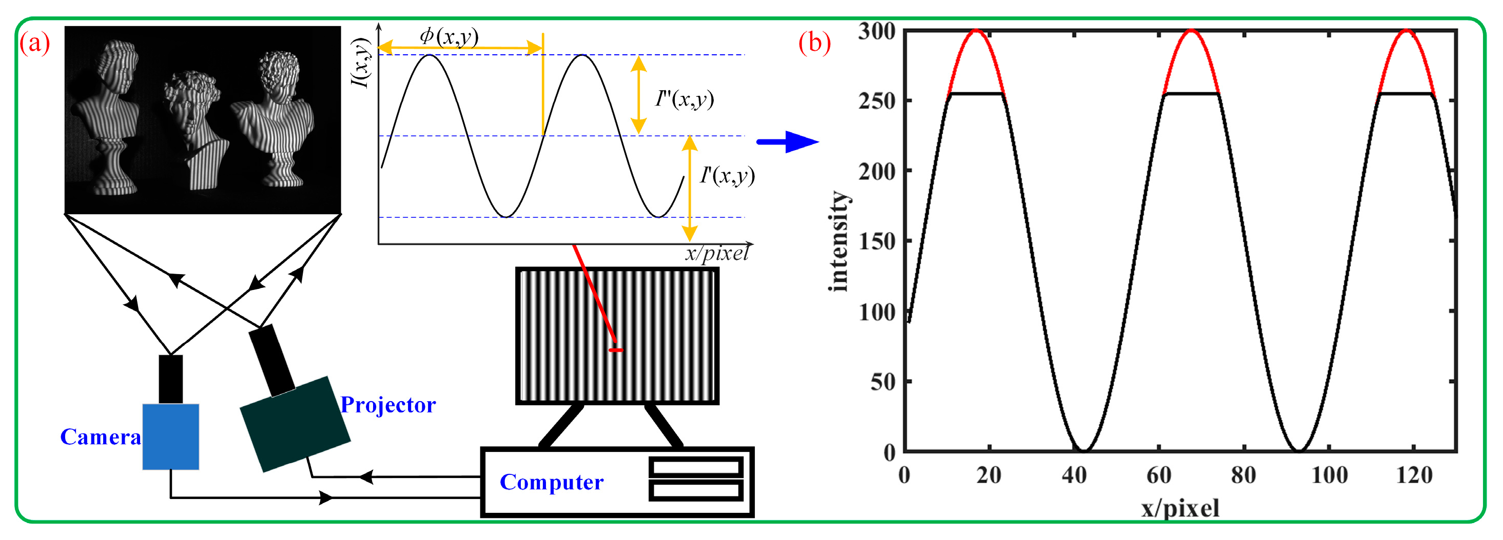
2.1. Principle of Phase-Shifting and Phase-Coding Method
2.2. The Proposed Algorithm Principle
2.2.1. Classification of Different Exposure Cases
2.2.2. Wrapped Phase, Texture, and Modulation Calculation
2.2.3. Unwrapped Phase Calculation
3. Experiments
3.1. Simulation Experiments
3.1.1. Normal Exposure Scene
3.1.2. Overexposure Scene
3.2. Physical Experiments
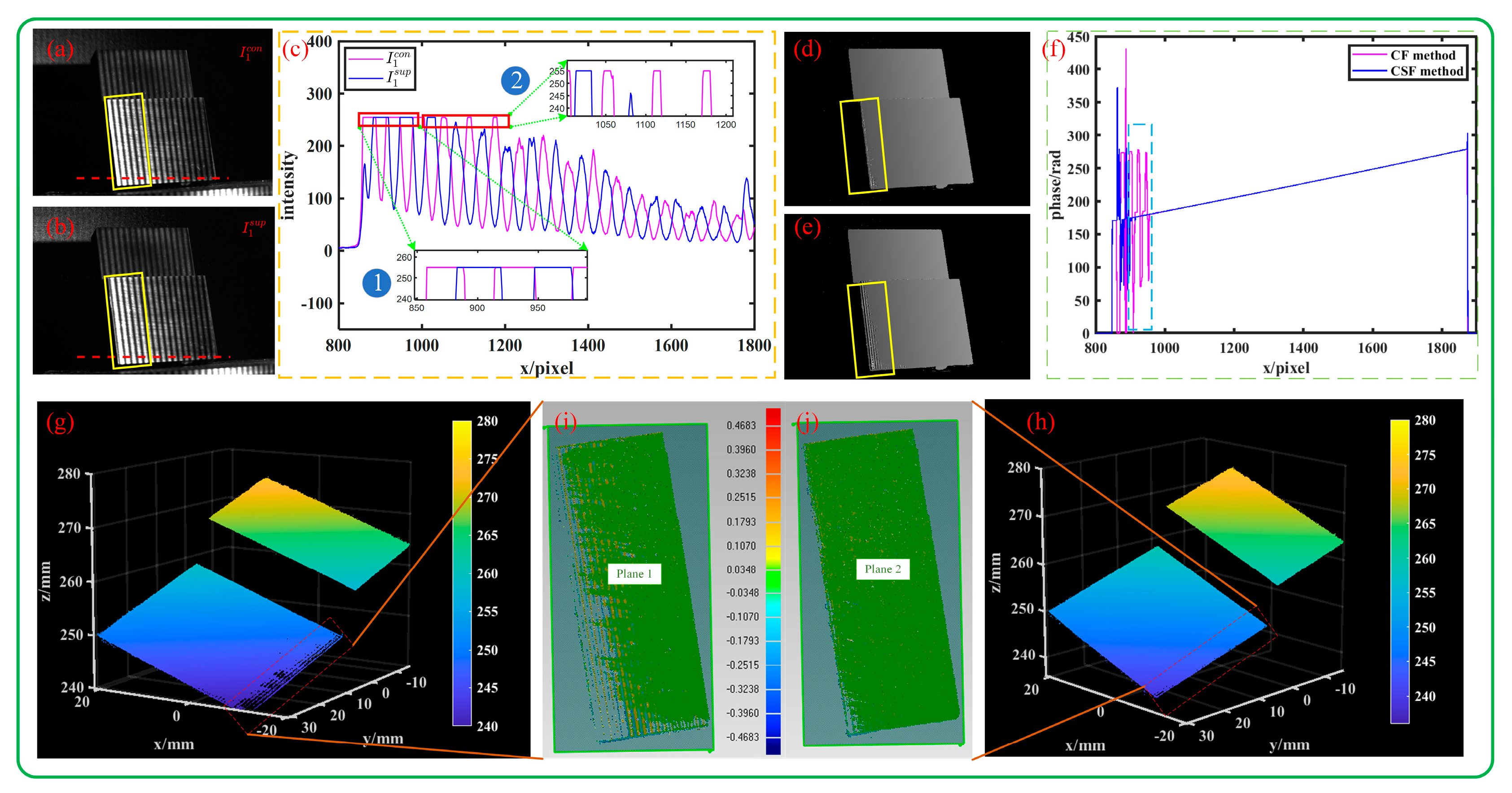
3.2.1. Accuracy Verification
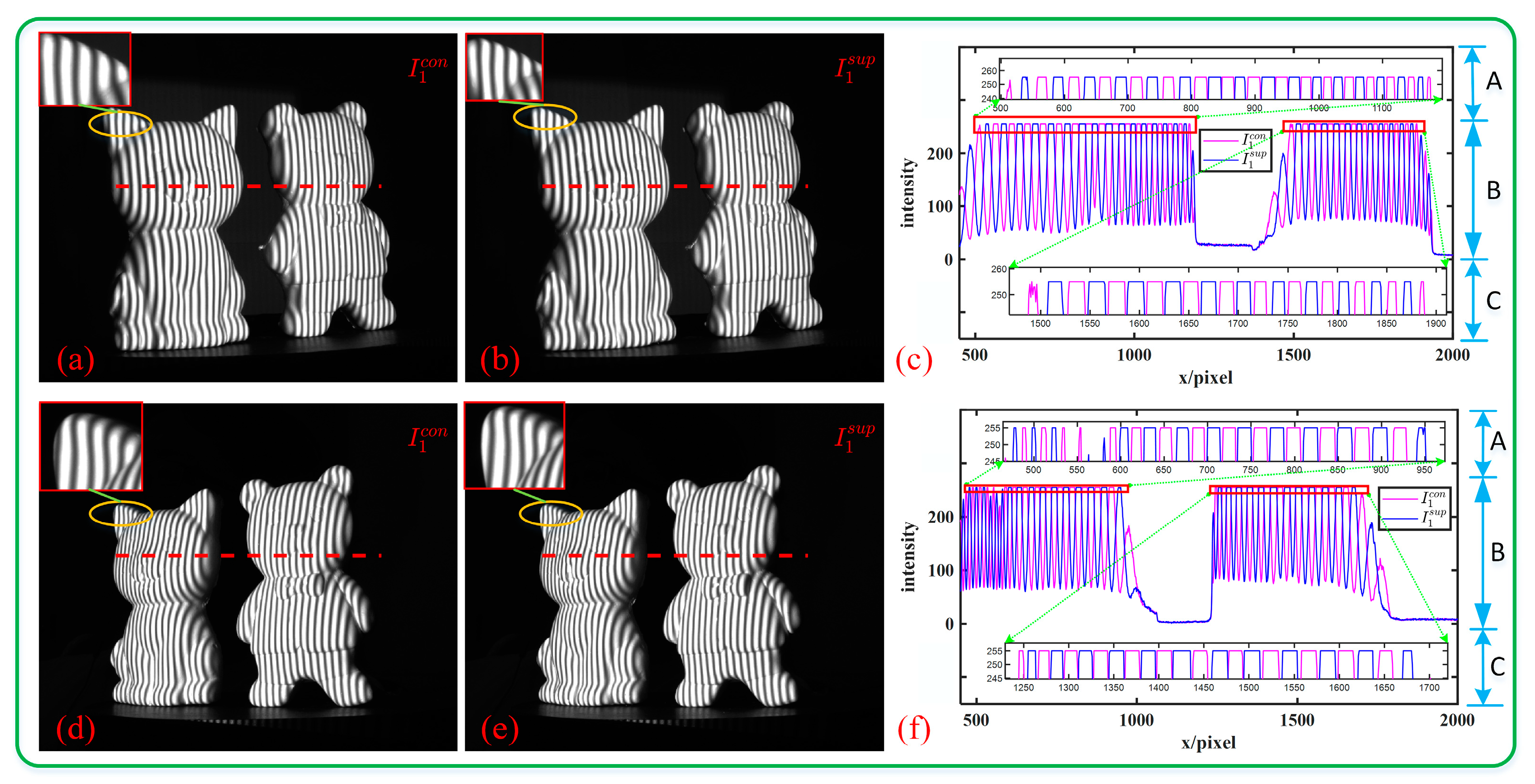
3.2.2. Isolated Object Measurement
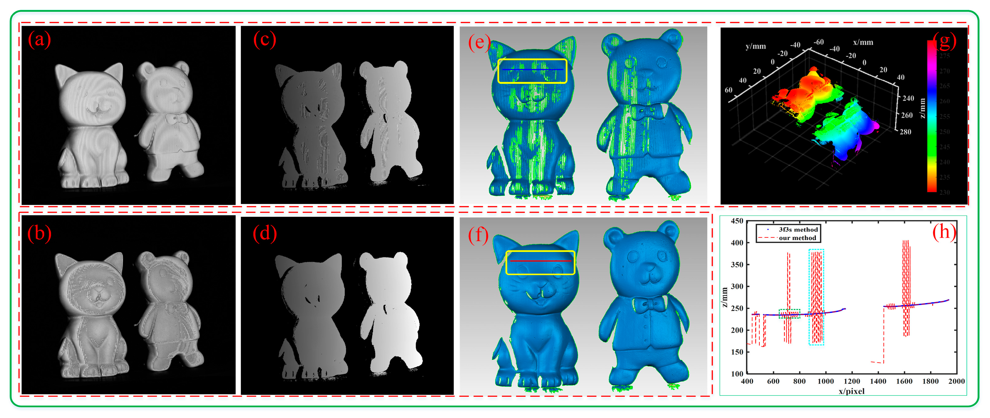
3.2.3. Measurement Completeness
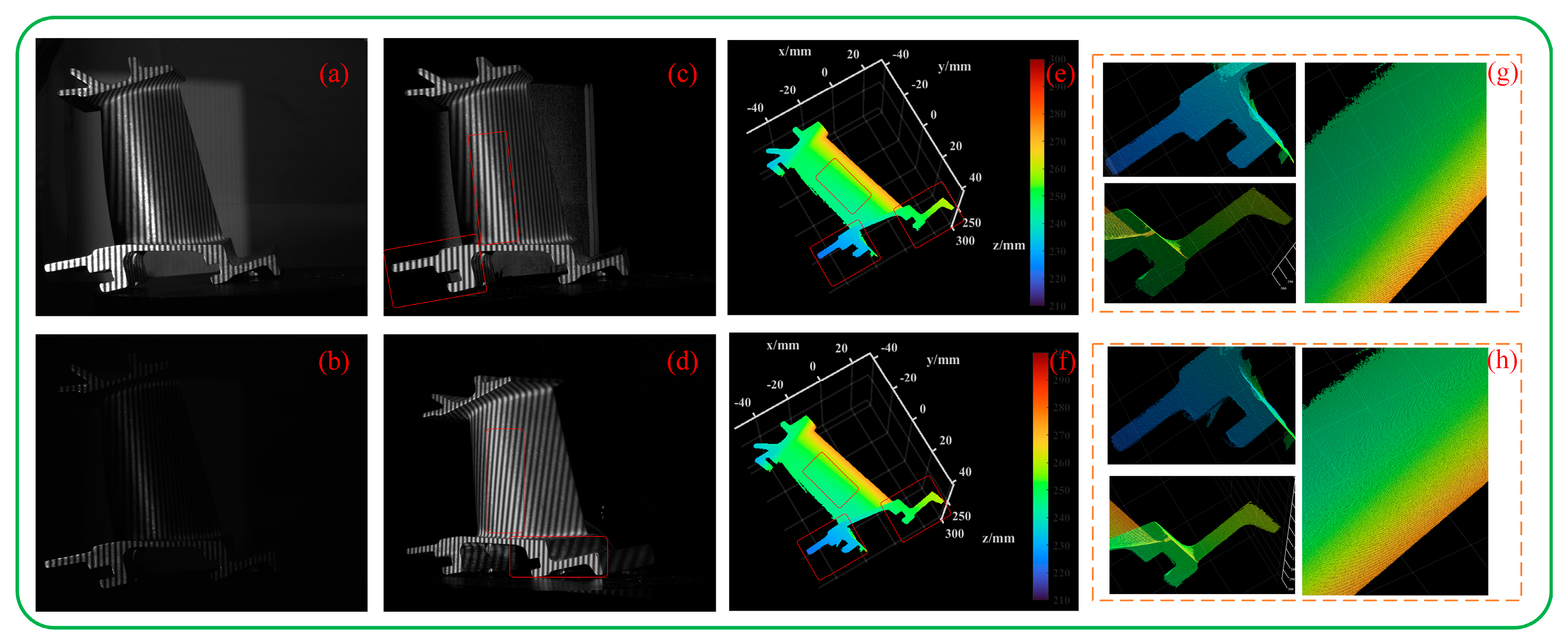
3.2.4. Measurement Flexibility
4. Conclusions
- (1)
- The fringe frequency of SPU is extended to improve measurement accuracy while inheriting the high measurement efficiency of the method. For binocular systems, several other techniques [36,37] can decrease the count of fringe patterns. Yet, they typically rely on complex, time-intensive spatial domain computations or embedding pattern methods. In contrast, our method is computationally simpler and easier to implement.
- (2)
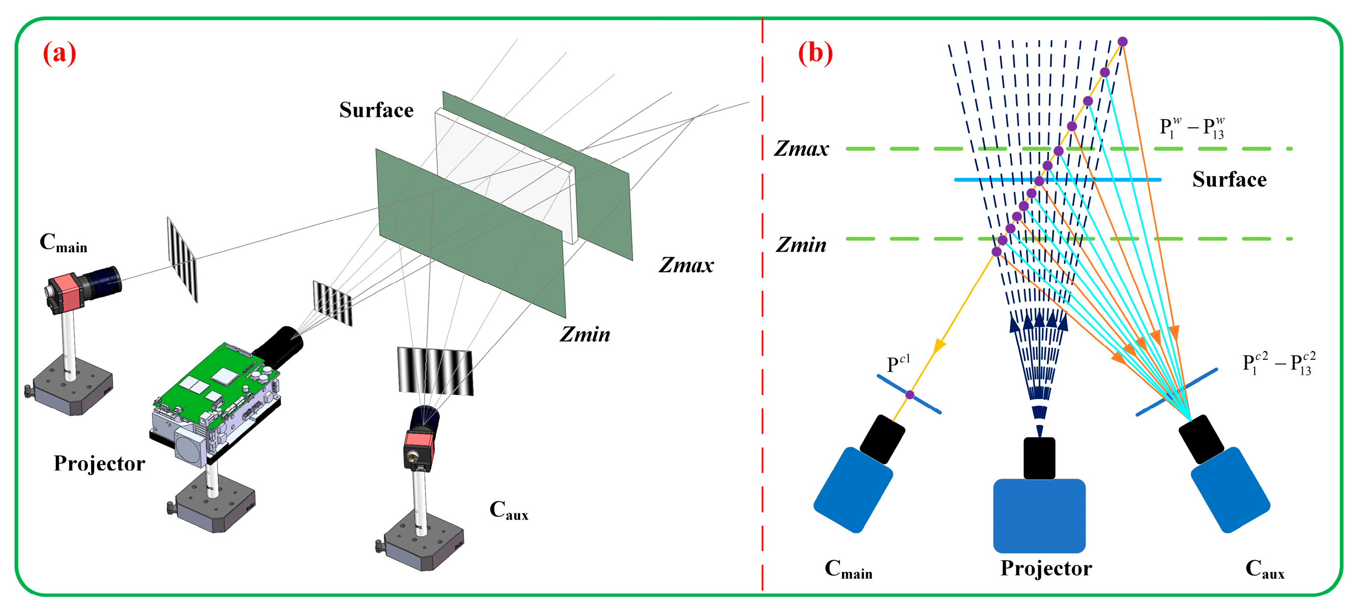
- Taking advantage of stereo cameras, phase recovery can be achieved by projecting an additional image on the basis of three-step phase shifting. There are also other methods that can perform phase unwrapping using only three or four fringes, but using π phase-shifting fringes to suppress the phase error in the overexposed area often leads to phase recovery failure, as seen in [38,39]. We only need to add four additional corresponding π phase-shifting fringes to deal with different overexposure situations. We reduced the number of fringes to 4/10 that of Jiang’s method. In addition, modulation calculation (for background removal) is added, and the dynamic range improvement capability is simply quantitatively analyzed (the dynamic range of the FPP system can be increased to twice that of the traditional method).
- (1)
- Since our method has good flexibility and uses a smaller number of patterns, the integration of real-time measurements into existing frameworks can be considered later.
- (2)
- Our method only amplifies the dynamic range twofold, so it is necessary to further expand the 3D measurement’s dynamic range.
Author Contributions
Funding
Institutional Review Board Statement
Informed Consent Statement
Data Availability Statement
Conflicts of Interest
References
- Frank Chen, G.M.; Mumin, S. Overview of three-dimensional shape measurement using optical methods. Opt. Eng. 2000, 39, 10–21. [Google Scholar]
- Blais, F. Review of 20 years of range sensor development. J. Electron. Imaging 2004, 13, 231–243. [Google Scholar] [CrossRef]
- Gorthi, S.S.; Rastogi, P. Fringe projection techniques: Whither we are? Opt. Lasers Eng. 2010, 48, 133–140. [Google Scholar] [CrossRef]
- Zuo, C.; Huang, L.; Zhang, M.; Chen, Q.; Asundi, A. Temporal phase unwrapping algorithms for fringe projection profilometry: A comparative review. Opt. Lasers Eng. 2016, 85, 84–103. [Google Scholar] [CrossRef]
- Zhang, S. High-speed 3D shape measurement with structured light methods: A review. Opt. Lasers Eng. 2018, 106, 119–131. [Google Scholar] [CrossRef]
- Zuo, C.; Feng, S.; Huang, L.; Tao, T.; Yin, W.; Chen, Q. Phase shifting algorithms for fringe projection profilometry: A review. Opt. Lasers Eng. 2018, 109, 23–59. [Google Scholar] [CrossRef]
- Feng, S.; Zuo, C.; Zhang, L.; Tao, T.; Hu, Y.; Yin, W.; Qian, J.; Chen, Q. Calibration of fringe projection profilometry: A comparative review. Opt. Lasers Eng. 2021, 143, 106622. [Google Scholar] [CrossRef]
- Palousek, D.; Omasta, M.; Koutny, D.; Bednar, J.; Koutecky, T.; Dokoupil, F. Effect of matte coating on 3D optical measurement accuracy. Opt. Mater. 2015, 40, 1–9. [Google Scholar] [CrossRef]
- Zhang, S.; Yau, S.-T. High dynamic range scanning technique. Opt. Eng. 2009, 48, 033604. [Google Scholar]
- Jiang, H.; Zhao, H.; Li, X. High dynamic range fringe acquisition: A novel 3-D scanning technique for high-reflective surfaces. Opt. Lasers Eng. 2012, 50, 1484–1493. [Google Scholar] [CrossRef]
- Feng, S.; Zhang, Y.; Chen, Q.; Zuo, C.; Li, R.; Shen, G. General solution for high dynamic range three-dimensional shape measurement using the fringe projection technique. Opt. Lasers Eng. 2014, 59, 56–71. [Google Scholar] [CrossRef]
- Ekstrand, L.; Zhang, S. Autoexposure for three-dimensional shape measurement using a digital-light-processing projector. Opt. Eng. 2011, 50, 123603. [Google Scholar] [CrossRef]
- Liu, G.-H.; Liu, X.-Y.; Feng, Q.-Y. 3D shape measurement of objects with high dynamic range of surface reflectivity. Appl. Opt. 2011, 50, 4557–4565. [Google Scholar] [CrossRef] [PubMed]
- Waddington, C.; Kofman, J. Analysis of measurement sensitivity to illuminance and fringe-pattern gray levels for fringe-pattern projection adaptive to ambient lighting. Opt. Lasers Eng. 2010, 48, 251–256. [Google Scholar] [CrossRef]
- Li, D.; Kofman, J. Adaptive fringe-pattern projection for image saturation avoidance in 3D surface-shape measurement. Opt. Express 2014, 22, 9887–9901. [Google Scholar] [CrossRef]
- Lin, H.; Gao, J.; Mei, Q.; He, Y.; Liu, J.; Wang, X. Adaptive digital fringe projection technique for high dynamic range three-dimensional shape measurement. Opt. Express 2016, 24, 7703–7718. [Google Scholar] [CrossRef]
- Chen, C.; Gao, N.; Wang, X.; Zhang, Z. Adaptive projection intensity adjustment for avoiding saturation in three-dimensional shape measurement. Opt. Commun. 2018, 410, 694–702. [Google Scholar] [CrossRef]
- Xu, S.; Feng, T.; Xing, F. 3D measurement method for high dynamic range surfaces based on adaptive fringe projection. IEEE Trans. Instrum. Meas. 2023, 72, 5013011. [Google Scholar]
- Zhou, P.; Wang, H.; Wang, Y.; Yao, C.; Lin, B. A 3D shape measurement method for high-reflective surface based on dual-view multi-intensity projection. Meas. Sci. Technol. 2023, 34, 075021. [Google Scholar] [CrossRef]
- Zhang, L.; Chen, Q.; Zuo, C.; Feng, S. High dynamic range and real-time 3D measurement based on a multi-view system. In Proceedings of the Second Target Recognition and Artificial Intelligence Summit Forum, Shenyang, China, 28–30 August 2019; SPIE: Bellingham, WA, USA, 2020; pp. 258–263. [Google Scholar]
- Hu, Q.; Harding, K.G.; Du, X.; Hamilton, D. Shiny parts measurement using color separation. In Proceedings of the Two-and Three-Dimensional Methods for Inspection and Metrology III, Boston, MA, USA, 24–26 October 2005; SPIE: Bellingham, WA, USA, 2005; pp. 125–132. [Google Scholar]
- Salahieh, B.; Chen, Z.; Rodriguez, J.J.; Liang, R. Multi-polarization fringe projection imaging for high dynamic range objects. Opt. Express 2014, 22, 10064–10071. [Google Scholar] [CrossRef]
- Nayar, S.K.; Fang, X.-S.; Boult, T. Separation of reflection components using color and polarization. Int. J. Comput. Vis. 1997, 21, 163–186. [Google Scholar] [CrossRef]
- Pei, X.; Ren, M.; Wang, X.; Ren, J.; Zhu, L.; Jiang, X. Profile measurement of non-Lambertian surfaces by integrating fringe projection profilometry with near-field photometric stereo. Measurement 2022, 187, 110277. [Google Scholar] [CrossRef]
- Chen, Y.; He, Y.; Hu, E. Phase deviation analysis and phase retrieval for partial intensity saturation in phase-shifting projected fringe profilometry. Opt. Commun. 2008, 281, 3087–3090. [Google Scholar] [CrossRef]
- Hu, E.; He, Y.; Chen, Y. Study on a novel phase-recovering algorithm for partial intensity saturation in digital projection grating phase-shifting profilometry. Optik 2010, 121, 23–28. [Google Scholar] [CrossRef]
- Chen, B.; Zhang, S. High-quality 3D shape measurement using saturated fringe patterns. Opt. Lasers Eng. 2016, 87, 83–89. [Google Scholar] [CrossRef]
- Jiang, C.; Bell, T.; Zhang, S. High dynamic range real-time 3D shape measurement. Opt. Express 2016, 24, 7337–7346. [Google Scholar] [CrossRef]
- Zhong, K.; Li, Z.; Shi, Y.; Wang, C.; Lei, Y. Fast phase measurement profilometry for arbitrary shape objects without phase unwrapping. Opt. Lasers Eng. 2013, 51, 1213–1222. [Google Scholar] [CrossRef]
- An, Y.; Hyun, J.-S.; Zhang, S. Pixel-wise absolute phase unwrapping using geometric constraints of structured light system. Opt. Express 2016, 24, 18445–18459. [Google Scholar] [CrossRef]
- Yin, W.; Feng, S.; Tao, T.; Huang, L.; Trusiak, M.; Chen, Q.; Zuo, C. High-speed 3D shape measurement using the optimized composite fringe patterns and stereo-assisted structured light system. Opt. Express 2019, 27, 2411–2431. [Google Scholar] [CrossRef]
- Zhang, S. Absolute phase retrieval methods for digital fringe projection profilometry: A review. Opt. Lasers Eng. 2018, 107, 28–37. [Google Scholar] [CrossRef]
- Wang, Y.; Zhang, S. Novel phase-coding method for absolute phase retrieval. Opt. Lett. 2012, 37, 2067–2069. [Google Scholar] [CrossRef] [PubMed]
- Liu, K.; Wang, Y.; Lau, D.L.; Hao, Q.; Hassebrook, L.G. Dual-frequency pattern scheme for high-speed 3-D shape measurement. Opt. Express 2010, 18, 5229–5244. [Google Scholar] [CrossRef] [PubMed]
- Tao, T.; Chen, Q.; Feng, S.; Qian, J.; Hu, Y.; Huang, L.; Zuo, C. High-speed real-time 3D shape measurement based on adaptive depth constraint. Opt. Express 2018, 26, 22440–22456. [Google Scholar] [CrossRef] [PubMed]
- Garcia, R.R.; Zakhor, A. Consistent stereo-assisted absolute phase unwrapping methods for structured light systems. IEEE J. Sel. Top. Signal Process. 2012, 6, 411–424. [Google Scholar] [CrossRef]
- Breitbarth, A.; Müller, E.; Kühmstedt, P.; Notni, G.; Denzler, J. Phase unwrapping of fringe images for dynamic 3D measurements without additional pattern projection. In Proceedings of the Dimensional Optical Metrology and Inspection for Practical Applications IV, Baltimore, MD, USA, 20–24 April 2015; SPIE: Bellingham, WA, USA, 2015; pp. 8–17. [Google Scholar]
- Wu, H.; Cao, Y.; An, H.; Li, Y.; Li, H.; Xu, C.; Yang, N. A novel phase-shifting profilometry to realize temporal phase unwrapping simultaneously with the least fringe patterns. Opt. Lasers Eng. 2022, 153, 107004. [Google Scholar] [CrossRef]
- Cai, B.; Zhang, L.; Wu, J.; Wang, M.; Chen, X.; Duan, M.; Wang, K.; Wang, Y. Absolute phase measurement with four patterns based on variant shifting phases. Rev. Sci. Instrum. 2020, 91, 065115. [Google Scholar] [CrossRef]


| Case | Overexposed Pattern(s) | Used Patterns |
|---|---|---|
| 1: No overexposed pattern | 1_1: None | |
| 2: An overexposed pattern | 2_1: | |
| 2_2: | ||
| 2_3: | ||
| 2_4: | ||
| 3: Two overexposed patterns | 3_1: | |
| 3_2: | ||
| 3_3: | ||
| 3_4: | ||
| 3_5: | ||
| 3_6: | ||
| 4: Three overexposed patterns | 4_1: | |
| 4_2: | ||
| 4_3: | ||
| 4_4: | ||
| 5: Four overexposed patterns | 5_1: |
| Case | Formula |
|---|---|
| 2_1 | |
| 2_2 | |
| 2_3 | |
| 2_4 | |
| 3_1 | |
| 3_2 | |
| 3_3 | |
| 3_4 | |
| 3_5 | |
| 3_6 | |
| 4_1 | |
| 4_2 | |
| 4_3 | |
| 4_4 | |
| 5_1 |
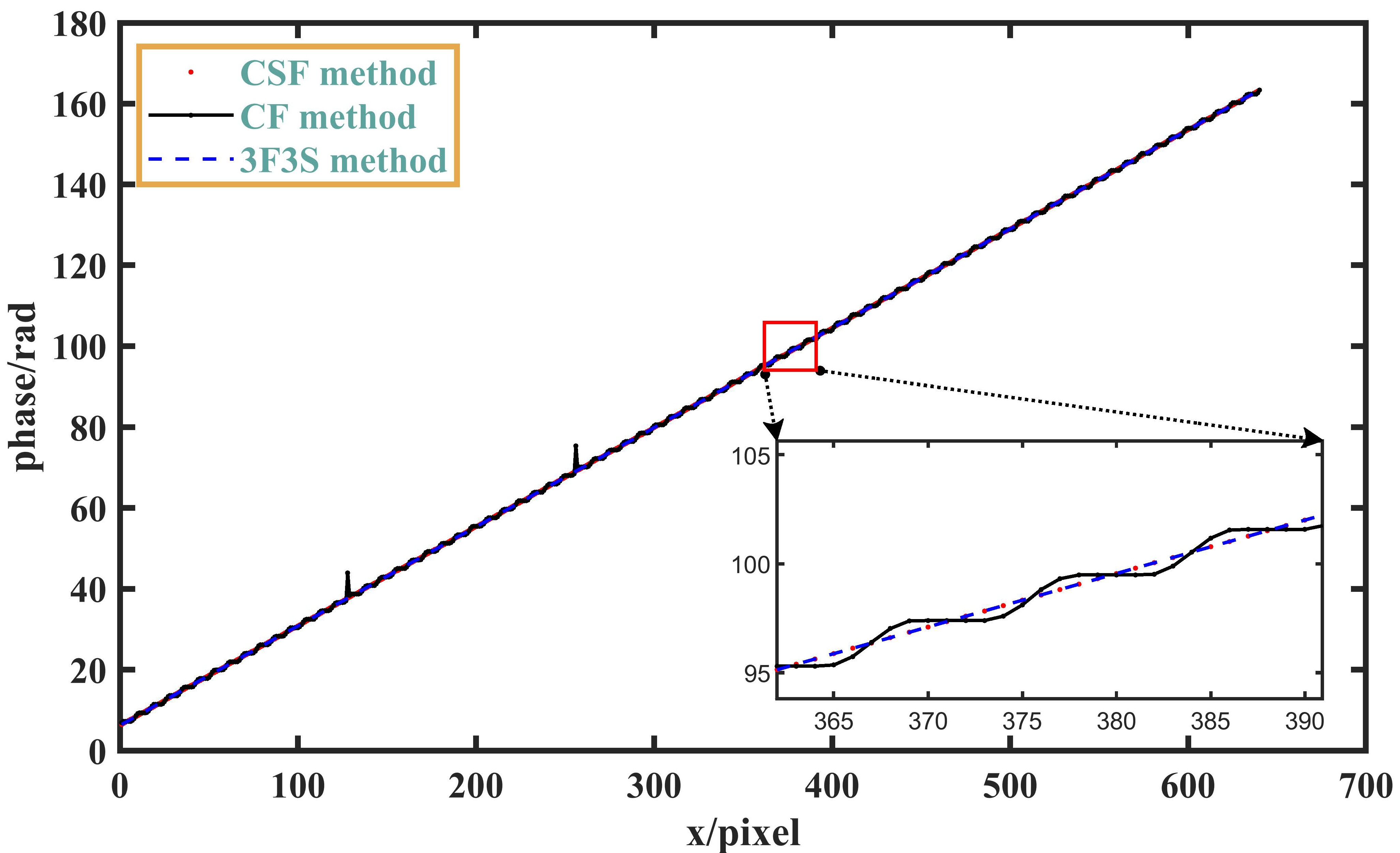
| SPU Method | Jiang’s Method [28] | CF Method | |
|---|---|---|---|
| 0.0397 | 0.0258 | 0.0259 | |
| 0.0194 | 0.0143 | 0.0150 | |
| 0.0241 | 0.0212 | 0.0203 |
| Jiang’s Method [28] | CF Method | CSF Method | |
|---|---|---|---|
| 0.0269 | 0.0405 | 0.0271 | |
| 0.0164 | 0.0266 | 0.0172 | |
| 0.0209 | 0.0204 | 0.0201 |
Disclaimer/Publisher’s Note: The statements, opinions and data contained in all publications are solely those of the individual author(s) and contributor(s) and not of MDPI and/or the editor(s). MDPI and/or the editor(s) disclaim responsibility for any injury to people or property resulting from any ideas, methods, instructions or products referred to in the content. |
© 2023 by the authors. Licensee MDPI, Basel, Switzerland. This article is an open access article distributed under the terms and conditions of the Creative Commons Attribution (CC BY) license (https://creativecommons.org/licenses/by/4.0/).
Share and Cite
Zhang, Y.; Sun, J. A Phase Retrieval Method for 3D Shape Measurement of High-Reflectivity Surface Based on π Phase-Shifting Fringes. Sensors 2023, 23, 8848. https://doi.org/10.3390/s23218848
Zhang Y, Sun J. A Phase Retrieval Method for 3D Shape Measurement of High-Reflectivity Surface Based on π Phase-Shifting Fringes. Sensors. 2023; 23(21):8848. https://doi.org/10.3390/s23218848
Chicago/Turabian StyleZhang, Yanjun, and Junhua Sun. 2023. "A Phase Retrieval Method for 3D Shape Measurement of High-Reflectivity Surface Based on π Phase-Shifting Fringes" Sensors 23, no. 21: 8848. https://doi.org/10.3390/s23218848