
Modified Two-Point Correction Method for Wide-Spectrum LWIR Detection System


Abstract
:1. Introduction
2. Traditional Two-Point Calibration Model
3. Modified TPC Method Based on Spectral Subdivision
3.1. Modified Model
3.2. Performance Analysis
4. Experiment
4.1. Experiment of TPC without Atmospheric Transmittance Filter
4.1.1. Black Body as the Target Image
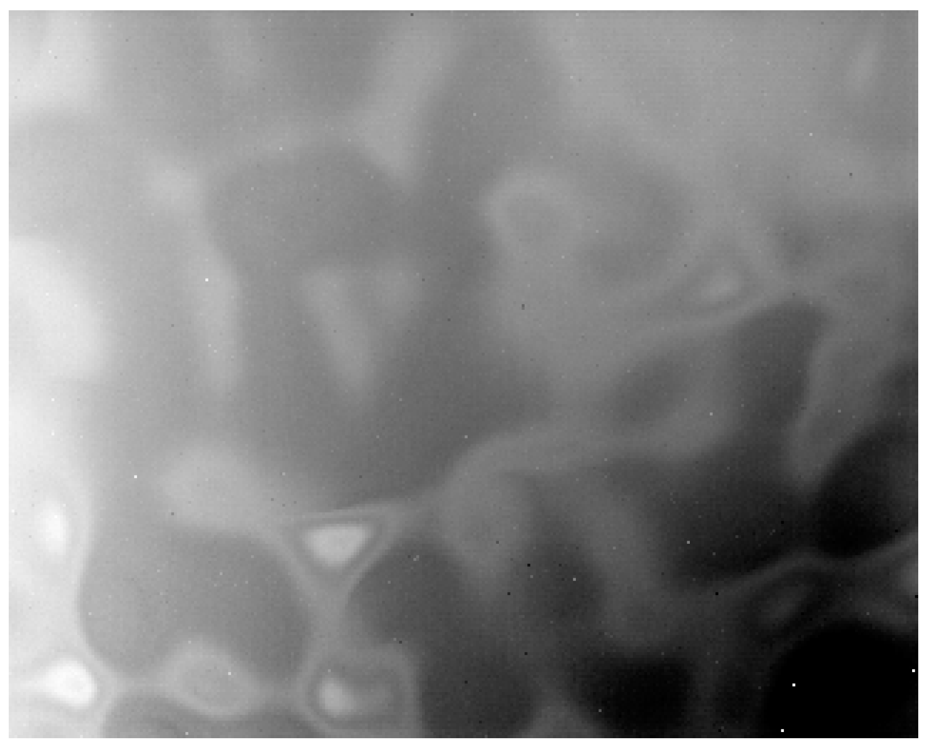
4.1.2. Sky Scene as Target Image
4.2. Experiment of TPC in Sky Scene with Two Sets Correction Coefficients
5. Discussion
6. Conclusions
Author Contributions
Funding
Institutional Review Board Statement
Informed Consent Statement
Data Availability Statement
Conflicts of Interest
References
- Fortunato, L.; Colombi, G.; Ondini, A.; Quaranta, C.; Giunti, C.; Sozzi, B.; Balzarotti, G. SKYWARD: The next Generation Airborne Infrared Search and Track. In Infrared Technology and Applications XLII; SPIE: Bellingham, WA, USA, 2016. [Google Scholar]
- Rogalski, A. Infrared Detectors: An Overview. Infrared Phys. Technol. 2002, 43, 187–210. [Google Scholar] [CrossRef]
- Page, G.A.; Carroll, B.D.; Pratt, A.E.; Randall, P.N. Long-Range Target Detection Algorithms for Infrared Search and Track. In Infrared Technology and Applications XXV; SPIE: Bellingham, WA, USA, 1999. [Google Scholar]
- Scribner, D.A.; Kruer, M.R.; Killiany, J.M. Infrared Focal Plane Array Technology. Proc. IEEE 1991, 79, 66–85. [Google Scholar] [CrossRef]
- Huo, L.; Zhou, D.; Wang, D.; Liu, R.; He, B. Staircase-Scene-Based Nonuniformity Correction in Aerial Point Target Detection Systems. Appl. Opt. 2016, 55, 7149–7156. [Google Scholar] [CrossRef]
- Wang, E.; Jiang, P.; Li, X.; Cao, H. Infrared Stripe Correction Algorithm Based on Wavelet Decomposition and Total Variation-Guided Filtering. J. Eur. Opt. Soc.-Rapid Publ. 2020, 16, 1. [Google Scholar] [CrossRef]
- Perry, D.L.; Dereniak, E.L. Linear Theory of Nonuniformity Correction in Infrared Staring Sensors. Opt. Eng. 1993, 32, 1854–1859. [Google Scholar] [CrossRef]
- Li, Z.; Shen, T.; Lou, S. Scene-Based Nonuniformity Correction Based on Bilateral Filter with Reduced Ghosting. Infrared Phys. Technol. 2016, 77, 360–365. [Google Scholar] [CrossRef]
- Zeng, J.; Sui, X.; Gao, H. Adaptive Image-Registration-Based Nonuniformity Correction Algorithm with Ghost Artifacts Eliminating for Infrared Focal Plane Arrays. IEEE Photonics J. 2015, 7, 6803016. [Google Scholar] [CrossRef]
- Hardie, R.C.; Hayat, M.M.; Armstrong, E.; Yasuda, B. Scene-Based Nonuniformity Correction with Video Sequences and Registration. Appl. Opt. 2000, 39, 1241–1250. [Google Scholar] [CrossRef] [PubMed]
- Zuo, C.; Chen, Q.; Gu, G.; Sui, X. Scene-Based Nonuniformity Correction Algorithm Based on Interframe Registration. J. Opt. Soc. America. A Opt. Image Sci. Vis. 2011, 28, 1164–1176. [Google Scholar] [CrossRef] [PubMed]
- Scribner, D.A.; Sarkady, K.A.; Kruer, M.R.; Caulfield, J.T.; Hunt, J.D.; Colbert, M.; Descour, M. Adaptive Retina-like Preprocessing for Imaging Detector Arrays. In Proceedings of the IEEE International Conference on Neural Networks, San Francisco, CA, USA, 28 March–1 April 1993; Volume 3, pp. 1955–1960. [Google Scholar]
- Qian, W.; Chen, Q.; Gu, G. Space Low-Pass and Temporal High-Pass Nonuniformity Correction Algorithm. Opt. Rev. 2010, 17, 24–29. [Google Scholar] [CrossRef]
- Zuo, C.; Chen, Q.; Gu, G.; Qian, W. New Temporal High-Pass Filter Nonuniformity Correction Based on Bilateral Filter. Opt. Rev. 2011, 18, 197–202. [Google Scholar] [CrossRef]
- Theocharous, E.; Ishii, J.; Fox, N.P. A Comparison of the Performance of a Photovoltaic HgCdTe Detector with That of Large Area Single Pixel QWIPs for Infrared Radiometric Applications. Infrared Phys. Technol. 2005, 46, 309–322. [Google Scholar] [CrossRef]
- Rogalski, A. Quantum Well Photoconductors in Infrared Detector Technology. J. Appl. Phys. 2003, 93, 4355–4391. [Google Scholar] [CrossRef]
- McClatchey, R.; Fenn, R.; Volz, F.; Garing, J. Optical Properties of the Atmosphere (Revised). Environ. Res. Pap. 1971, 411, 100. [Google Scholar] [CrossRef]
- Williams, G.M.; Wames, R.E.D. Numerical Simulation of HgCdTe Detector Characteristics. J. Electron. Mater. 1995, 24, 1239–1248. [Google Scholar] [CrossRef]
- Quan, Z.J.; Li, Z.F.; Hu, W.D.; Ye, Z.H.; Hu, X.N.; Lu, W. Parameter Determination from Resistance-Voltage Curve for Long-Wavelength HgCdTe Photodiode. J. Appl. Phys. 2006, 100, 084503. [Google Scholar] [CrossRef]
- Mooney, J.M.; Sheppard, F.D.; Ewing, W.S.; Ewing, J.E.; Silverman, J. Responsivity Nonuniformity Limited Performance Of Infrared Staring Cameras. Opt. Eng. 1989, 28, 281151. [Google Scholar] [CrossRef]
- Mooney, J.M.; Shepherd, F.D. Characterizing IR FPA Nonuniformity and IR Camera Spatial Noise. Infrared Phys. Technol. 1996, 37, 595–606. [Google Scholar] [CrossRef]
- Huang, F.; Xueju, S.; Liu, J.; Li, G.; Ying, J. Research on Radiometric Calibration for Super Wide-Angle Staring Infrared Imaging System. Infrared Phys. Technol. 2013, 61, 9–13. [Google Scholar] [CrossRef]
- Mermelstein, M.; Snail, K.; Priest, R. Spectral and Radiometric Calibration of Midwave and Longwave Infrared Cameras. Opt. Eng. 2000, 39, 106–113. [Google Scholar] [CrossRef]
- Liang, K.; Yang, C.; Peng, L.; Zhou, B. Nonuniformity Correction Based on Focal Plane Array Temperature in Uncooled Long-Wave Infrared Cameras without a Shutter. Appl. Opt. 2017, 56, 884. [Google Scholar] [CrossRef] [PubMed]
- Sui, X.; Chen, Q.; Gu, G. A Novel Non-Uniformity Evaluation Metric of Infrared Imaging System. Infrared Phys. Technol. 2013, 60, 155–160. [Google Scholar] [CrossRef]
- Zhou, D.; Wang, D.; Huo, L.; Liu, R.; Jia, P. Scene-Based Nonuniformity Correction for Airborne Point Target Detection Systems. Opt. Express 2017, 25, 14210. [Google Scholar] [CrossRef] [PubMed]


| Parameters | Value |
|---|---|
| Spectral band | 7.7–11.3 μm |
| Material | HgCdTe |
| Resolution | 320 × 256 |
| NETD | 19 mK |
| Bit depth | 14 bit |
| Focal length | 38 mm |
| F/# | 2 |
| Parameters | Value |
|---|---|
| Average slope | 117.87 |
| Linear fitted slope | 118.30 |
| Linearity difference | 0.36% |
| Description | Requirement |
|---|---|
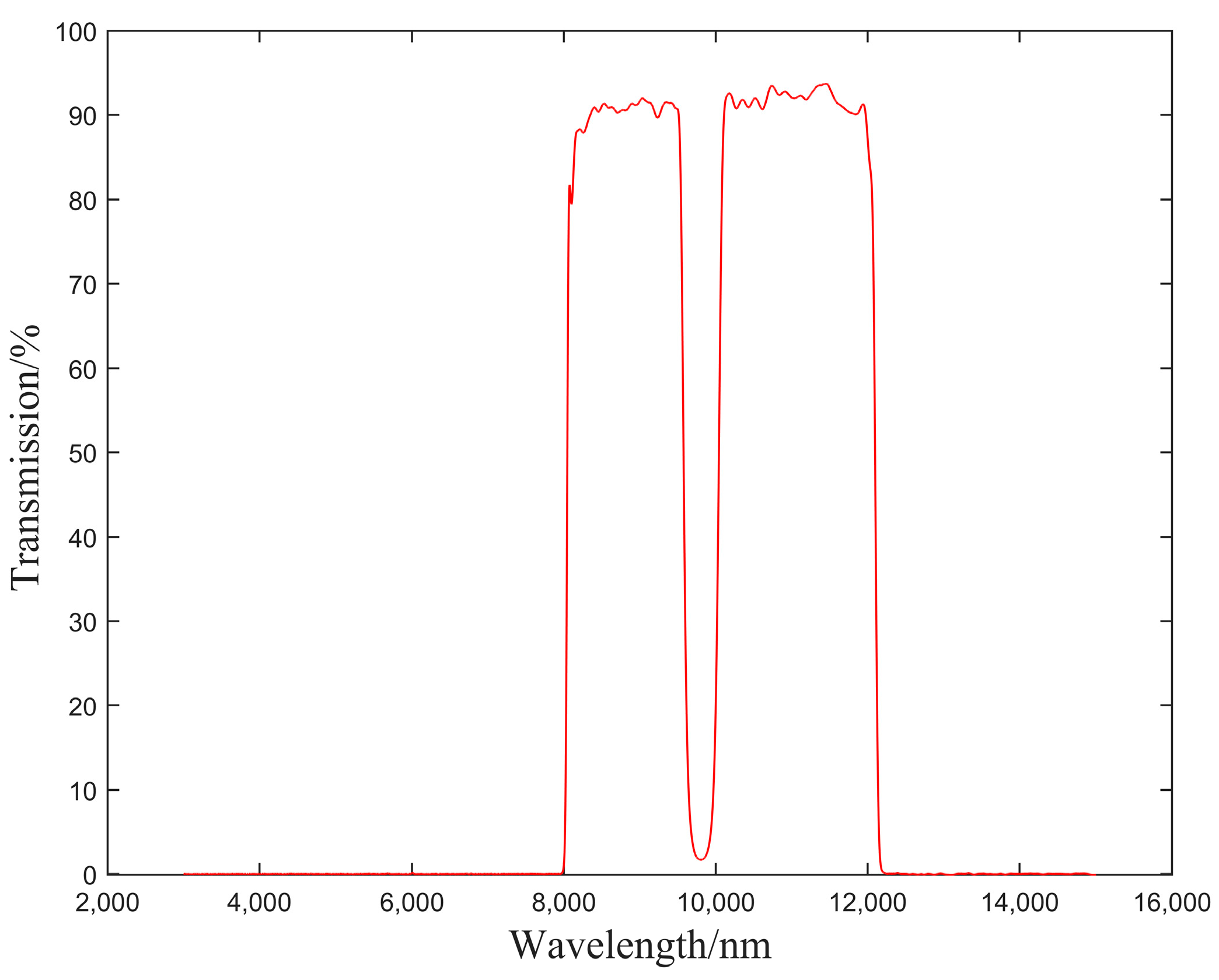
| Transmission | T > 85 ± 1% (for the range 8.0–9.5 µm) |
| Transmission | T > 85 ± 1% (for the range 9.9–11.7 µm) |
| Reflection Average | R > 94 ± 1% T < 5%(for the range 9.6–9.8 µm) |
| Out-of-Band Blocking | T < 0.1% average 3–15 µm |
| Size 1 | Diameter1 = 25 mm |
| Clear Aperture 1 | C1 ≥ 20 mm |
| Size 2 | Diameter2 = 16 mm |
| Clear Aperture 2 | C2 ≥ 13 mm |
| Thickness | 1 mm nominal |
| Surface Quality | E-E per Mil-C-48497A (60/40 equivalent) |
| Pinholes | Best practices to minimize pinholes, no guarantee |
| Construction | Unmounted, single substrate |
| TWF Error | TWF < 1/4 wave P-V per inch—prior to coating customer accepted 2 waves P-V |
| Parallelism | Parallelism < 20 arc seconds |
| Substrate material | Optical grade germanium |
| Corrected Image without Filter | Corrected Image with Filter | |
|---|---|---|
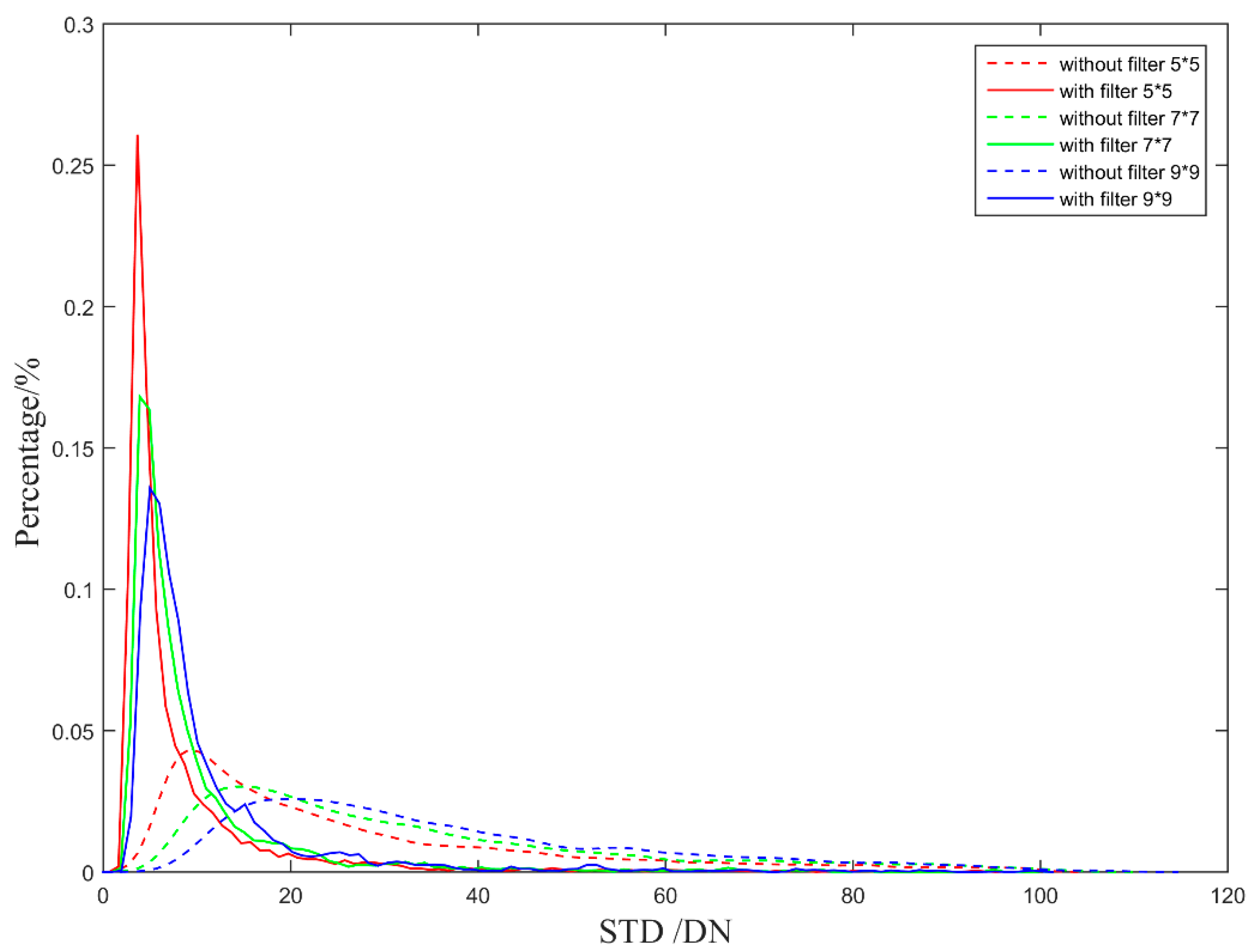
| Local STD (5 × 5) | 9.19 | 3.64 |
| Local STD (7 × 7) | 13.91 | 3.89 |
| Local STD (9 × 9) | 19.57 | 4.98 |
| Average grayscale | 7922.2 | 7922.1 |
| Local NU (5 × 5) | 0.116% | 0.0459% |
| Local NU (7 × 7) | 0.176% | 0.0491% |
| Local NU (9 × 9) | 0.247% | 0.0629% |
Disclaimer/Publisher’s Note: The statements, opinions and data contained in all publications are solely those of the individual author(s) and contributor(s) and not of MDPI and/or the editor(s). MDPI and/or the editor(s) disclaim responsibility for any injury to people or property resulting from any ideas, methods, instructions or products referred to in the content. |
© 2023 by the authors. Licensee MDPI, Basel, Switzerland. This article is an open access article distributed under the terms and conditions of the Creative Commons Attribution (CC BY) license (https://creativecommons.org/licenses/by/4.0/).
Share and Cite
Zhang, D.; Sun, H.; Wang, D.; Liu, J.; Chen, C. Modified Two-Point Correction Method for Wide-Spectrum LWIR Detection System. Sensors 2023, 23, 2054. https://doi.org/10.3390/s23042054
Zhang D, Sun H, Wang D, Liu J, Chen C. Modified Two-Point Correction Method for Wide-Spectrum LWIR Detection System. Sensors. 2023; 23(4):2054. https://doi.org/10.3390/s23042054
Chicago/Turabian StyleZhang, Di, He Sun, Dejiang Wang, Jinghong Liu, and Cheng Chen. 2023. "Modified Two-Point Correction Method for Wide-Spectrum LWIR Detection System" Sensors 23, no. 4: 2054. https://doi.org/10.3390/s23042054
APA StyleZhang, D., Sun, H., Wang, D., Liu, J., & Chen, C. (2023). Modified Two-Point Correction Method for Wide-Spectrum LWIR Detection System. Sensors, 23(4), 2054. https://doi.org/10.3390/s23042054