The data extracted from the brain signals of patients with epilepsy represent an essential example of imbalanced medical data. Most of these signals are normal and do not contain an epileptic seizure. In this implementation, a real and big dataset was used as a data stream to evaluate the quality of the proposed method. The evaluation included a number of the popular adaptive classifiers and performance measures that are most used for data stream classification tasks. This section begins with a brief explanation of the used dataset and the framework, then describes the obtained results.
4.2. Experimental Results
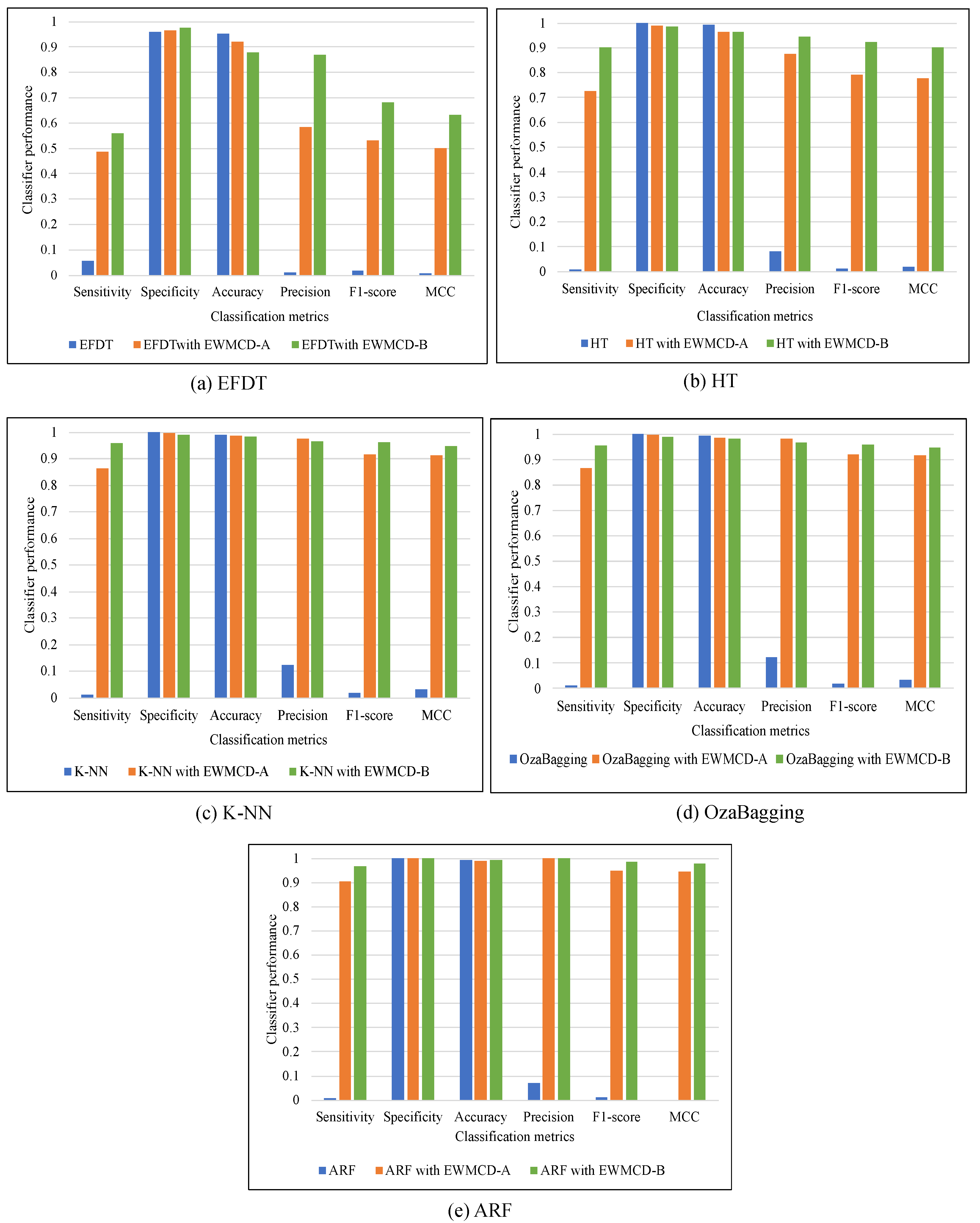
The effectiveness of EWMCD-A and EWMCD-B has been evaluated using a performance comparison of five adaptive classifiers with six metrics. The classifiers were Extreme Fast Decision Tree (EFDT), Hoeffding Tree, K Nearest Neighbor (K-NN), OzaBagging, and Adaptive Random Forest (ARF). The metrics were Sensitivity (i.e., True Positive Rate), Specificity (i.e., True Negative Rate), Accuracy, Precision, F-Score, and Matthews Correlation Coefficient (MCC).
The comparison in
Table 1 and
Table 2 showed that the performance of all classifiers had recognizable improvement using both EWMCD-A and EWMCD-B. Except for the accuracy metric, which tends most to the major class, Precision, F-Score, and MCC confirm this improvement which becomes more apparent in the K-NN classifier. K-NN mainly relies on selecting the closest data points for classification. On the other hand, the ensemble classifiers OzaBagging and ARF benefited more than single model algorithms (i.e., EFDT, Hoeffding Tree), as illustrated in
Figure 4. The advantage of ensemble models is resulted from building many base classifiers using different subsets from the given data.
A significant improvement in the performance of ARF can be seen in
Table 3. Sensitivity increased from 0.0067 to 0.9016, 0.9682 for EWMCD-A and EWMCD-B, preserving the high value of Specificity in both simultaneously. As a result of this accurate classifying of both classes, the values of Precision enhanced using EWMCD-B from 0.0700 to 0.9996 and F1-score from 0.0122 to 0.9837, representing a notable improvement compared with our previous method SAW. MCC metric can have a more reliable evaluation with an imbalanced dataset [
31]; its value increased to 0.9790 using EWMCD-B after it was zero without using the proposed models.
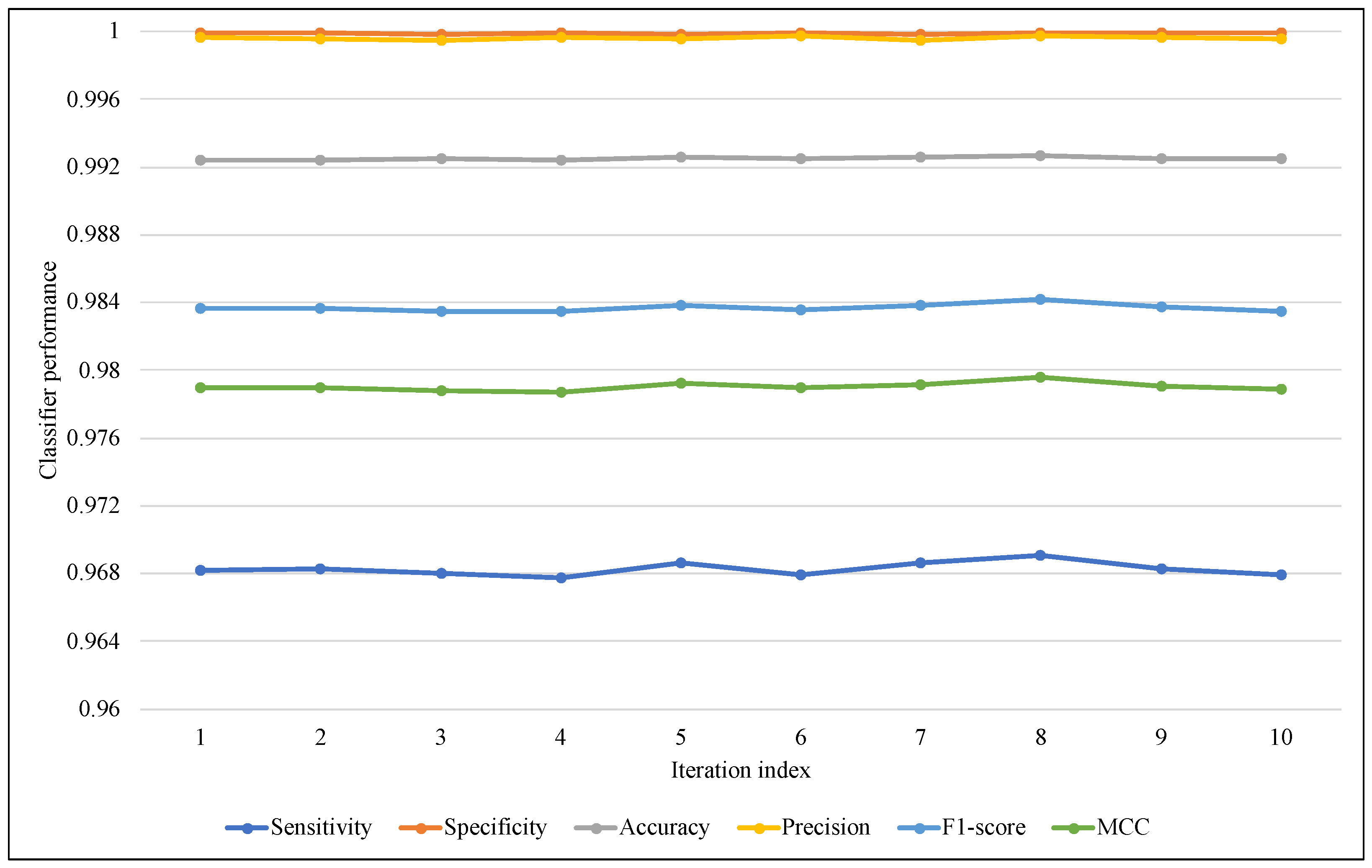
The proposed models use a random function for generating the random vector while creating a synthetic itemset. To avoid the effects of this randomness, in addition to ARF classifier randomness, the test-then-train process has been repeated 10 times, and the average of these iterations was used in comparisons of this section.
Figure 5 and
Figure 6 illustrate the performance of ARF for all iterations with the six metrics, in
Figure 5 of EWMCD-A, although there were slight changes in Sensitivity, the three measures of Precision, F1-score, and MCC remained stable in the 10 trials. In
Figure 6 of EWMCD-B, more stability of the ARF classifier can be observed in terms of Sensitivity and the other five metrics as well.
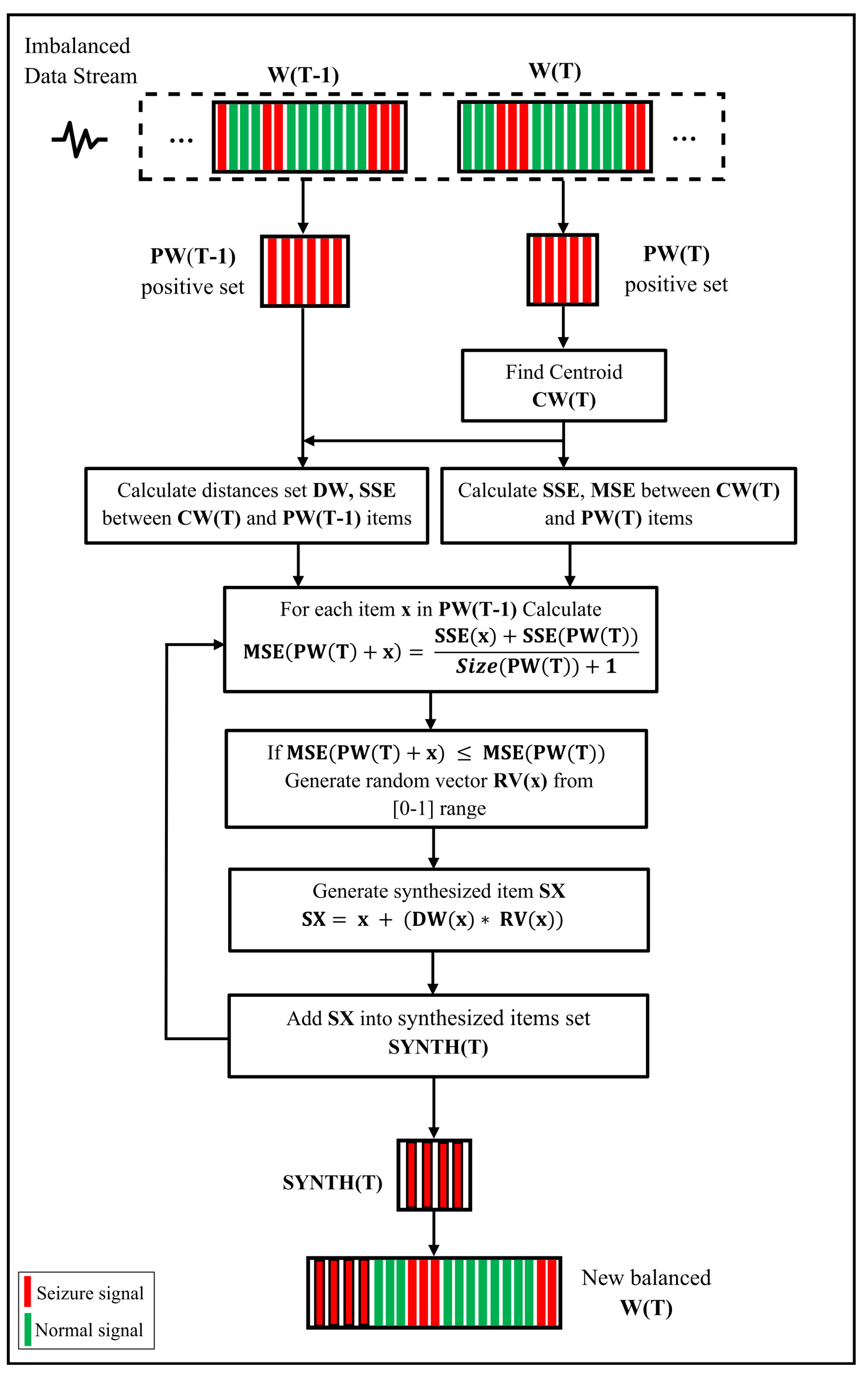
The evaluation also included changing the range of random vector values from [0–1] to [0–0.5] and [0.5–1]. The random vector RV(T) values will be limited between zero and 0.5 in the first range; as a result, the synthetic generated data point will be closer to the centroid CW(T). On the other hand, this point will be toward the MCD item in case of using the second range [0.5–1].
Table 4 showed that ARF had more accurate results using the [0–0.5] range. However, in all the results of other tables and figures, the range [0–1] is used as in the original SMOTE algorithm.
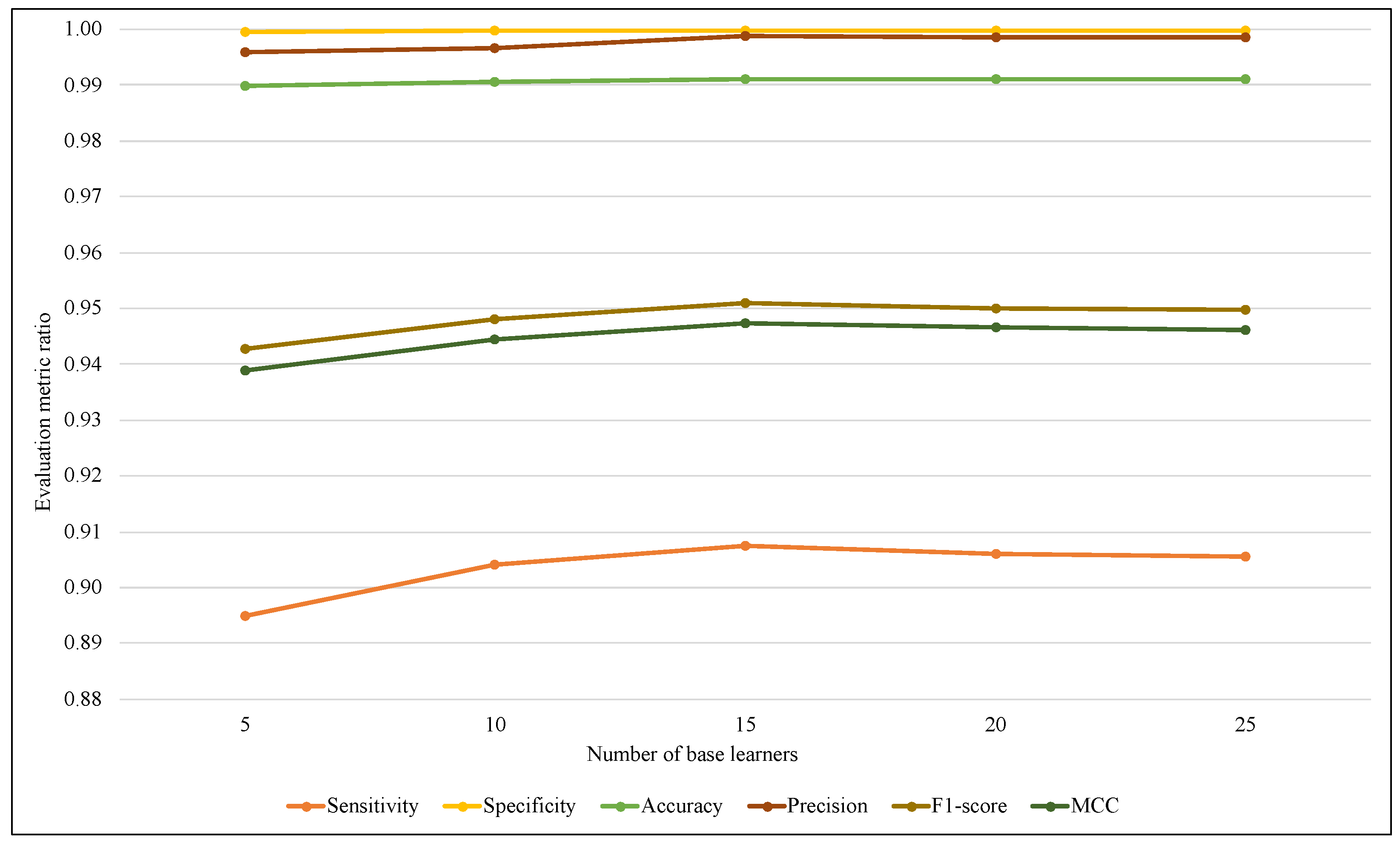
The ensemble size is considered one of the most affected parameters on the ARF classifier that refers to the base learners’ amount. Therefore, another comparison has been performed using different values of ARF ensemble size with the two models.
Figure 7 illustrates that using EWMCD-A, ARF effectiveness increased when the number of base learners increased from 5 to 15, then it started to decrease. EWMCD-B had a more stable performance with different values of the ensemble size from 5 to 25, as illustrated in
Figure 8, and the best-obtained results were using 25 base learners.
Another significant observation in this implementation is how and when the size of the proposed elastic window changed and how the performance of the ARF classifier responded to this change.
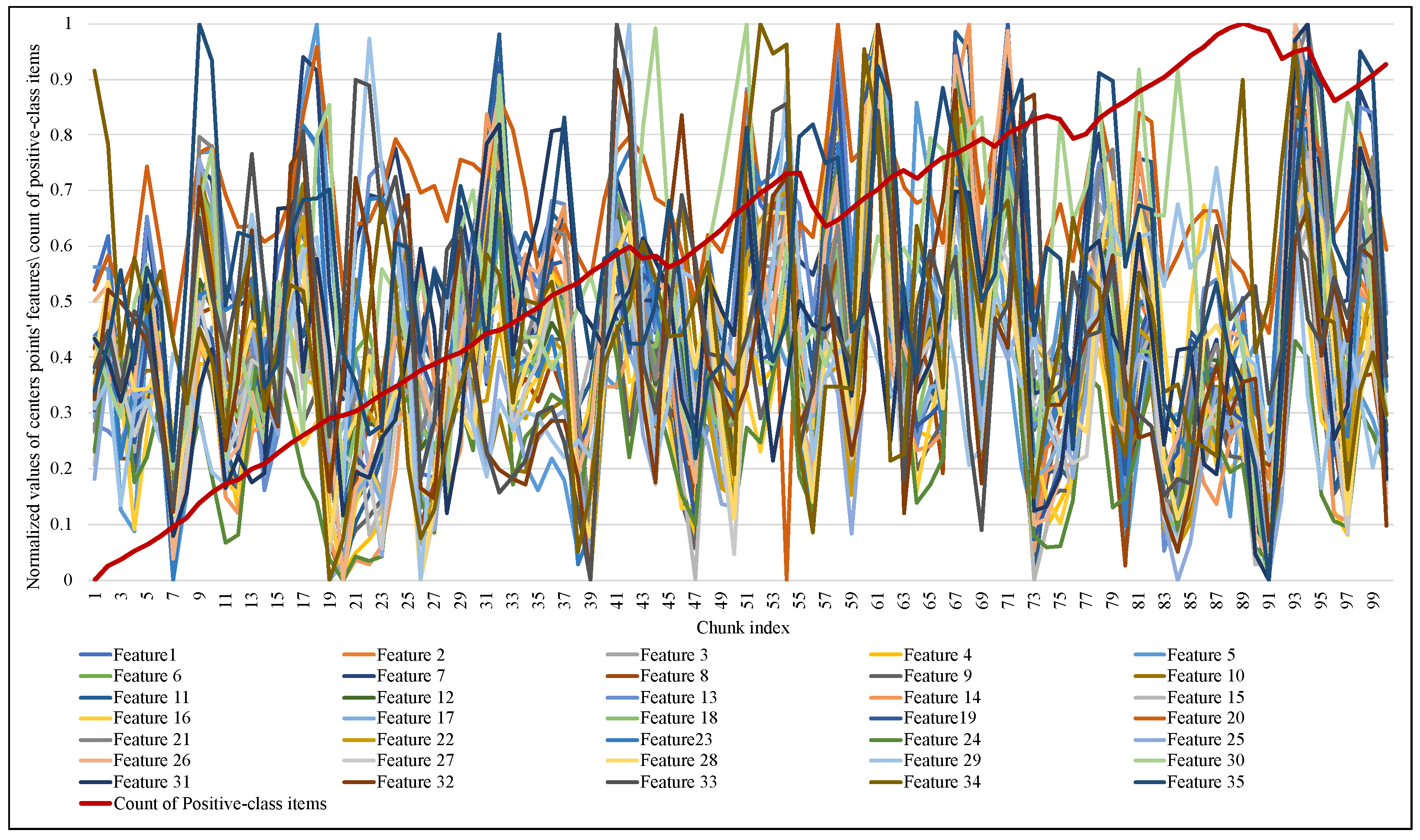
Figure 9 and
Figure 10 illustrate the normalized values of the MCD itemset centroid’s features for each data chunk during the training of ARF. Regarding the EWMCD-A model in
Figure 9, three major abrupt can be seen in the size of the window in chunk indexes (19, 56, 91). The sudden change in data distribution of the current window reflects on the position of its centroid, thereby reducing the number of elements from the previous window that can be added to the virtual cluster while maintaining the distortion level. In
Figure 10, the EWMCD-B model had a more stable window size that grew steadily from the first chunk until chunk 41, where it started to have some drift changes.
The rigorous adapting of EWMCD-A and its intensive changes in window size led to a notable response in ARF classifier performance in terms of Sensitivity, F1-score, and MCC while processing the first 40 chunks. After that, ARF had a stable performance, although there were many changes in window size, as
Figure 11 showed. On the other hand, EWMCD-B did not suffer similar difficulties, as
Figure 12 showed that the classifier had stable performance after chunk 13, up to the end of data stream classification in chunk 100, depending on the values of the six performance measures.
Due to the importance of analyzing and classifying EEG data, the Sienna dataset has been used in many research papers.
Table 5 includes a comparison of the performance of the proposed models with four of the most recent studies, noting that the metrics in this table were limited to what has been used in those studies, and their classification models were built as a batch classifier. Regarding accuracy and Specificity, both models EWMCD-A and EWMCD-B had the best results compared with other studies. Furthermore, both models had the best results regarding Sensitivity except for research work [
32].
The last comparison in the implementation was related to the required computational time for both the training and inference process.
Figure 13 illustrates the training time of the ARF classifier using SAW, EWMCD-A, and EWMCD-B models. Despite the increase in the time required by using the EWMCD-A model compared to the original ARF and SAW time, this is due to the number of calculations for measuring distances and generating synthetic data points. The significant increase in training time of the EWMCD-B is related to the accumulative increase in the number of positive-class instances, thereby increasing distances calculations of and modifying the classifier.
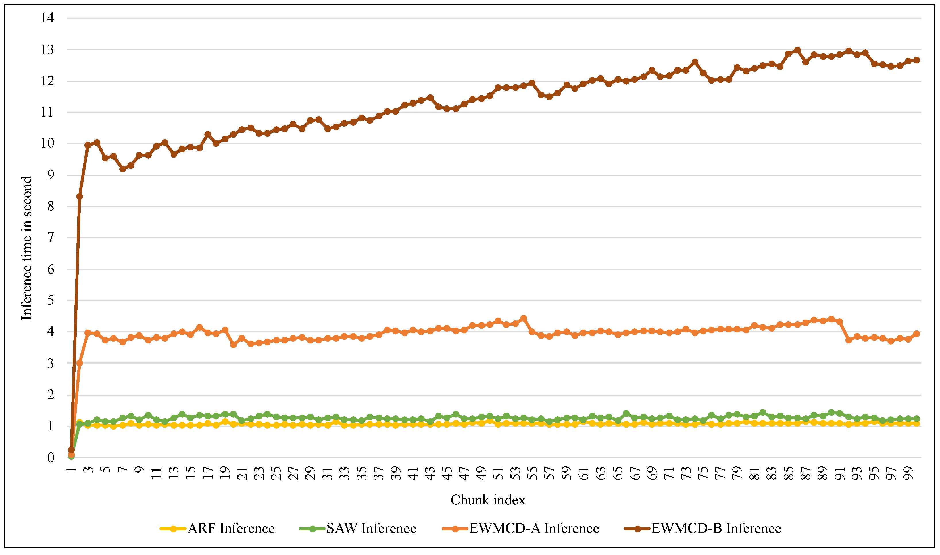
Figure 14 shows similar differences in the time required for the inference process using the proposed models. Although this process does not require calculating distances, using the test-then-train method requires testing each element in the window before training it. Thus, increasing the number of elements means increasing the time needed for inference. Despite this increase, the average time required to infer each instance did not exceed 0.0022 s in EWMCD-A and 0.0054 s in EWMCD-B. This performance provides a quick response to critical medical conditions, such as the early stages of an epileptic seizure, to avoid exacerbating the health condition.


