

Passive Wireless Pressure Gradient Measurement System for Fluid Flow Analysis

 ,
,
Abstract
:1. Introduction
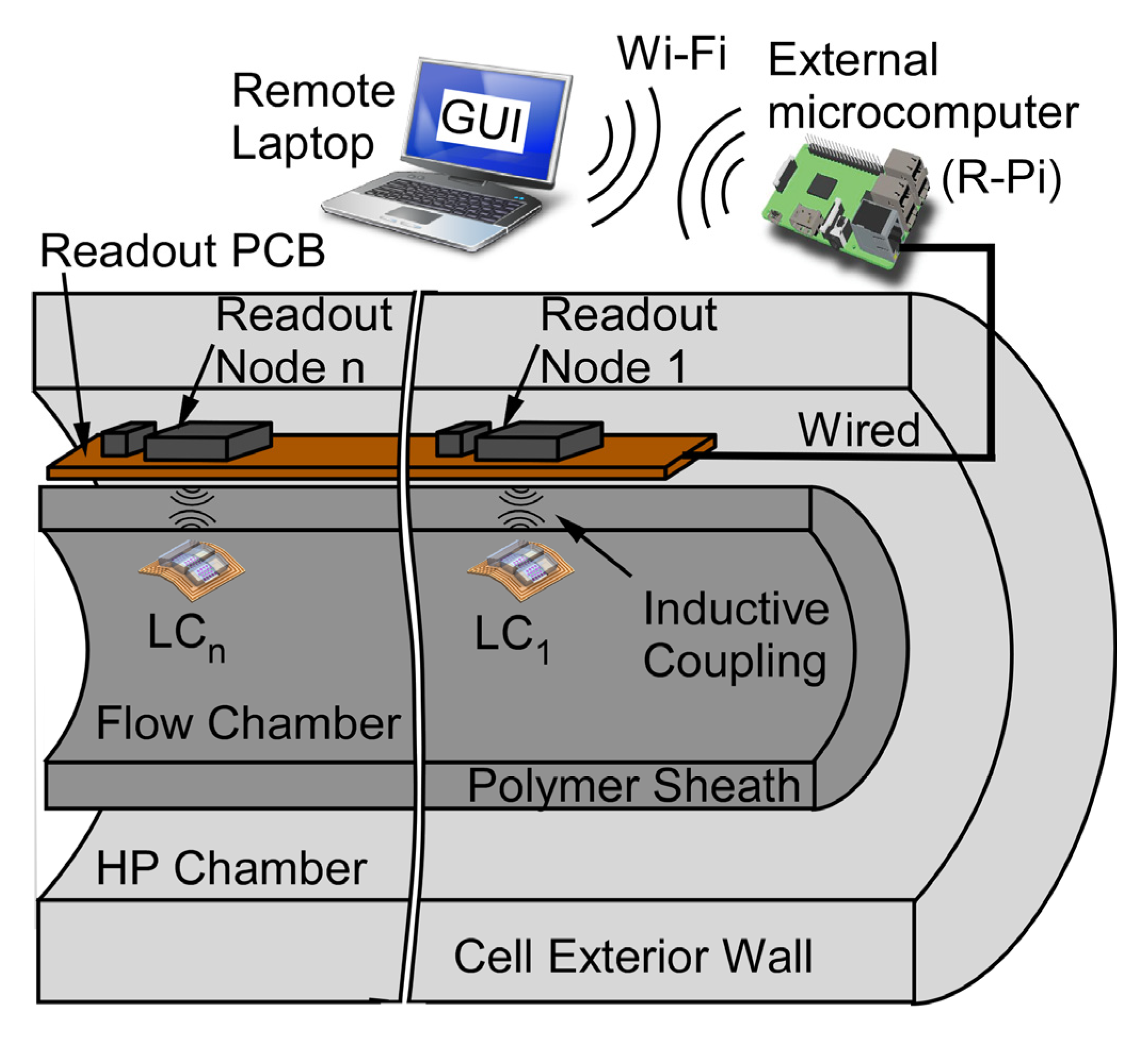
2. System Design
2.1. LC Sensor Model
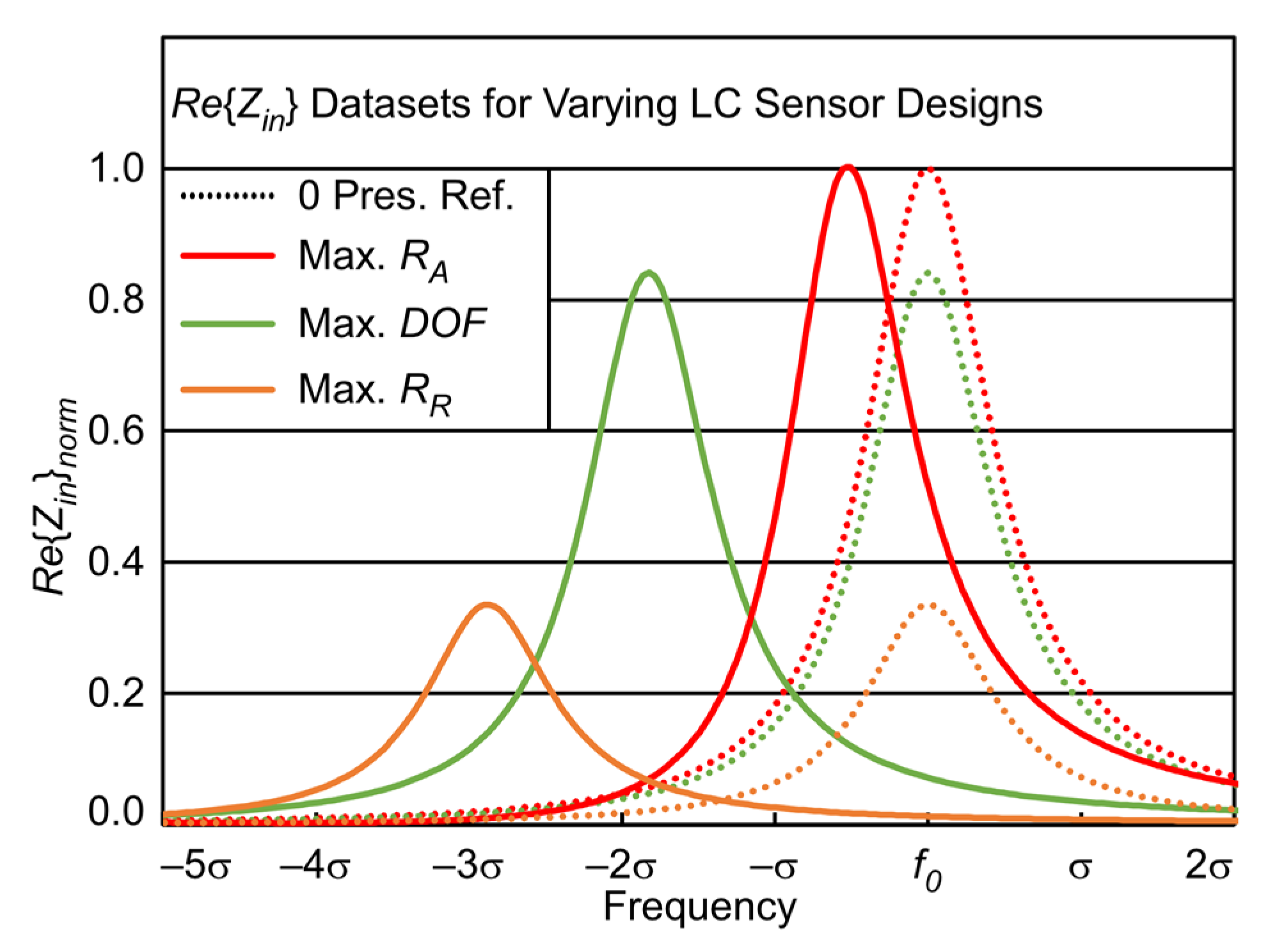
2.2. Design Methodology
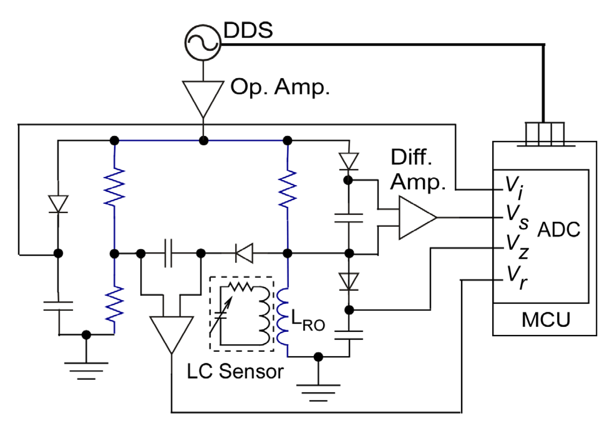
2.3. Readout Circuit
3. System Fabrication and Packaging
3.1. LC Sensor Fabrication
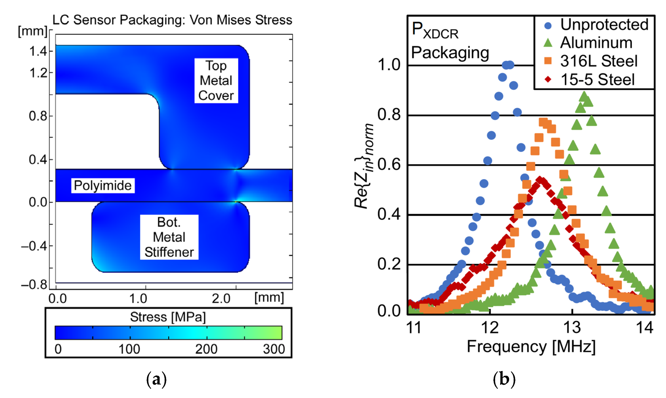
3.2. LC Sensor Packaging
3.3. Readout Circuit Fabrication
4. Test Results
4.1. LC Sensor Readout System
4.2. Dynamic Pressure Response and Flow Resolution
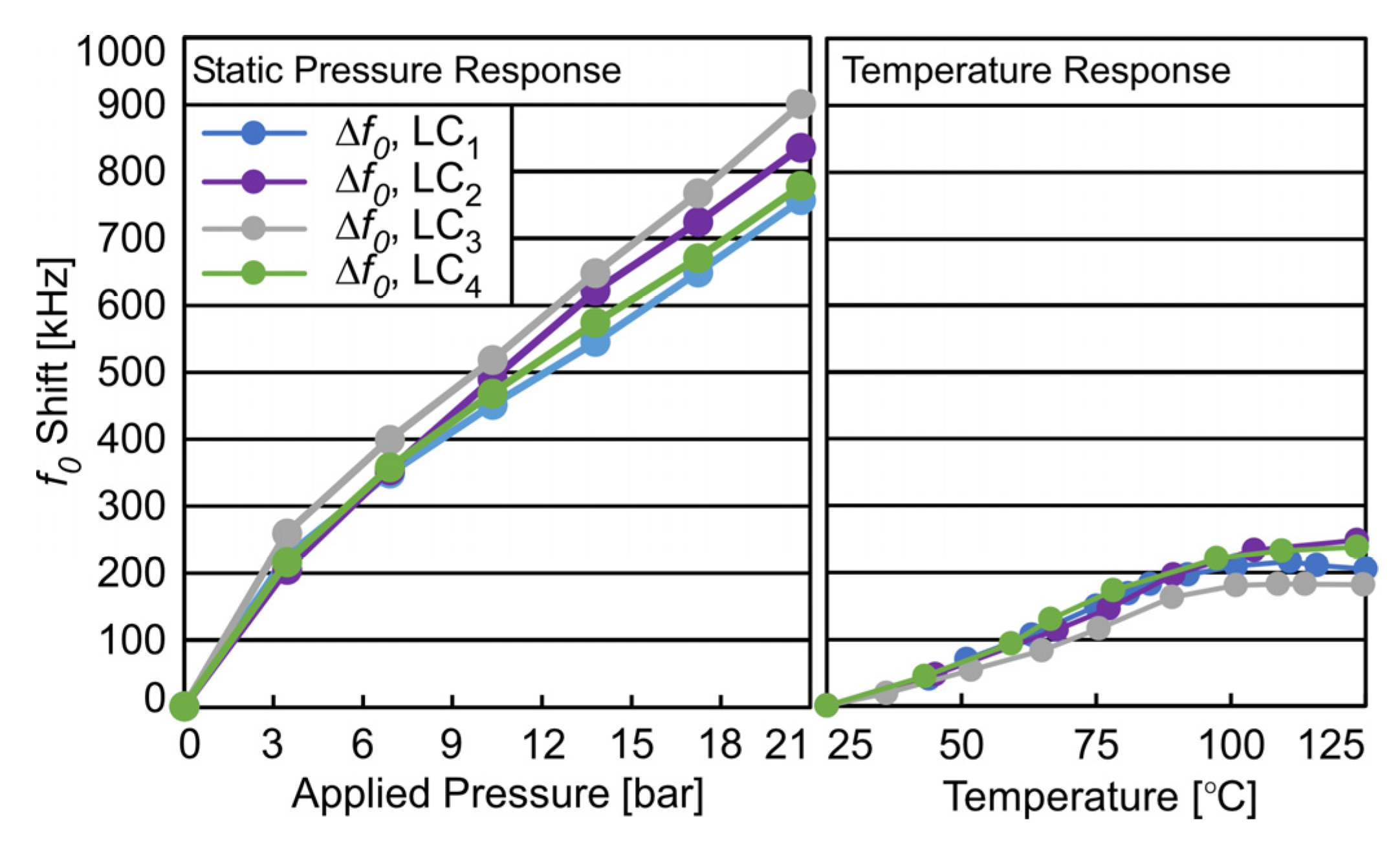
4.3. System Static Pressure and Thermal Response
4.4. Conversion of Resonant Frequency to Pressure
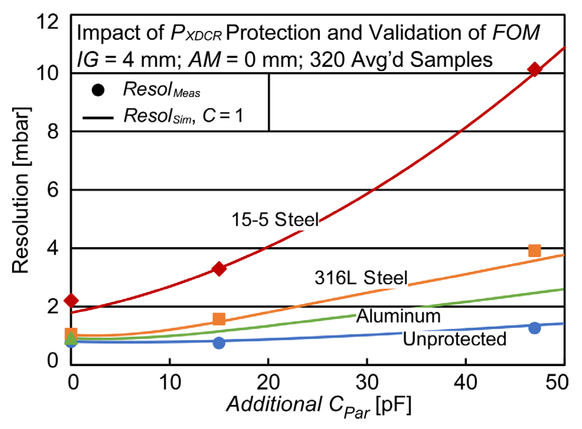
4.5. Pressure Resolution Enhancement
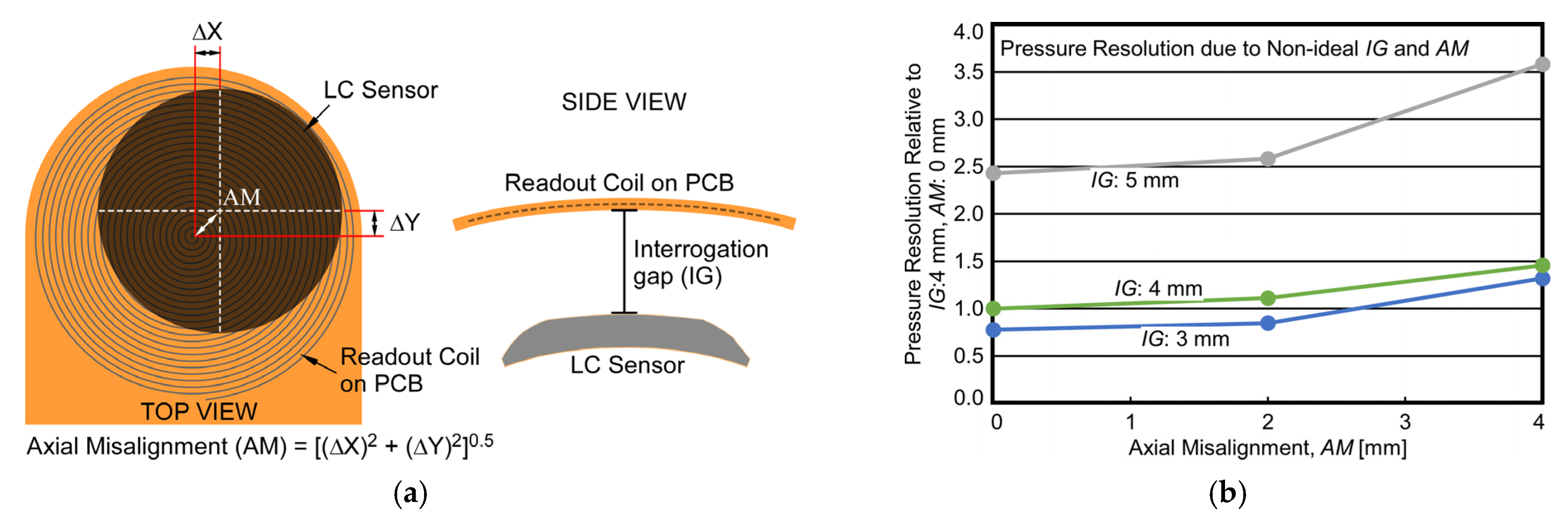
4.6. System Deployment Variations
5. Discussion
6. Conclusions and Summary
7. Patents
Author Contributions
Funding
Institutional Review Board Statement
Data Availability Statement
Acknowledgments
Conflicts of Interest
References
- Park, J.S.; Gianchandani, Y. A low cost batch-sealed capacitive pressure sensor. In Proceedings of the IEEE/ASME 12th International Conference on Micro Electro Mechanical Systems (MEMS 99), Orlando, FL, USA, 17–21 January 1999; pp. 82–87. [Google Scholar]
- Grimes, C.A.; Jain, M.K.; Singh, R.S.; Cai, Q.; Mason, A.; Takahata, K.; Gianchandani, Y. Magnetoelastic microsensors for environmental monitoring. In Proceedings of the IEEE/ASME 14th International Conference on Micro Electro Mechanical Systems (MEMS 01), Interlaken, Switzerland, 21–25 January 2001; pp. 278–281. [Google Scholar]
- Takahata, K.; DeHennis, A.; Wise, K.; Gianchandani, Y. A wireless microsensor for monitoring flow and pressure in a blood vessel utilizing a dual-inductor antenna stent and two pressure sensors. In Proceedings of the IEEE/ASME 17th International Conference on Micro Electro Mechanical Systems (MEMS 04), Maastricht, The Netherlands, 25–29 January 2004; pp. 216–219. [Google Scholar]
- Chapman, D.; Trybula, W. Meeting the Challenges of Oilfield Exploration using Intelligent Micro and Nano-Scale Sensors. In Proceedings of the IEEE 12th International Conference on Nanotechnology, Birmingham, UK, 20–23 August 2012; pp. 20–23. [Google Scholar]
- Fleming, W. Overview of automotive sensors. IEEE Sens. J. 2001, 1, 296–308. [Google Scholar] [CrossRef] [Green Version]
- Wu, C.H.; Zorman, C.; Mehregany, M. Fabrication and testing of bulk micromachined silicon carbide piezoresistive pressure sensors for high temperature applications. IEEE Sens. J. 2006, 6, 316–324. [Google Scholar]
- Chavan, A.V.; Wise, K.D. Batch-processed vacuum-sealed capacitive pressure sensors. J. Microelectromech. Syst. 2001, 10, 580–588. [Google Scholar] [CrossRef] [Green Version]
- Gianchandani, Y.; Wilson, C.; Park, J.-S. Micromachined pressure sensors: Devices, interface circuits, and performance limits. In The MEMS Handbook; Gad-el-Hak, M., Ed.; CRC Press: Boca Raton, FL, USA, 2006; pp. 1–44. [Google Scholar]
- Benken, A.; Gianchandani, Y. Passive Wireless Pressure Sensing for Gastric Manometry. Micromachines 2019, 10, 868. [Google Scholar] [CrossRef] [Green Version]
- O’Neal, C.B.; Malshe, A.P.; Singh, S.B.; Brown, W.D.; Eaton, W.P. Challenges in the packaging of MEMS. In Proceedings of the International Symposium on Advanced Packaging Materials, Processes, Properties and Interfaces, Braselton, GA, USA, 14–17 March 1999; pp. 41–47. [Google Scholar]
- Savazzi, S.; Guardiano, S.; Spagnolini, U. Wireless sensor network modeling and deployment challenges in oil and gas refinery plants. Int. J. Distrib. Sens. Netw. 2013, 9. [Google Scholar] [CrossRef]
- Khan, W.Z.; Aalsalem, M.Y.; Gharibi, W.; Arshad, Q. Oil and Gas monitoring using Wireless Sensor Networks: Requirements, issues and challenges. In Proceedings of the IEEE International Conference on Radar, Antenna, Microwave, Electronics, and Telecommunications (ICRAMET), Jakarta, Indonesia, 3–5 October 2016; pp. 31–35. [Google Scholar]
- Hester, J.; Sorber, J. The future of sensing is batteryless, intermittent, and awesome. In Proceedings of the 15th ACM Conference on Embedded Network Sensor Systems, New York, NY, USA, 6–8 November 2017; pp. 1–6. [Google Scholar]
- Samaun; Wise, K.D.; Angell, J.B. An IC piezoresistive pressure sensor for biomedical instrumentation. IEEE Trans. Biomed. Eng. 1973, 20, 101–109. [Google Scholar] [CrossRef]
- Sander, S.; Knutti, J.W.; Meindl, J.D. A monolithic capacitive pressure sensor with pulse-period output. IEEE Trans. Electron. Devices 1980, 27, 927–930. [Google Scholar] [CrossRef]
- Bui, T.; Dinh, T.; Terebessy, T. Pressure sensor based on bipolar discharge corona configuration. Sens. Actuators A Phys. 2016, 237, 81–90. [Google Scholar]
- Luo, X.; Gianchandani, Y.B. A Microdischarge-Based Pressure Sensor Fabricated Using Through-Wafer Isolated Bulk-Silicon Lead Transfer. J. Microelectromech. Syst. 2018, 27, 365–373. [Google Scholar] [CrossRef]
- Ma, W.; Jiang, Y.; Hu, J.; Jiang, L.; Zhang, T. Microelectromechanical system-based, high-finesse, optical fiber Fabry–Perot interferometric pressure sensors. Sens. Actuators A Phys. 2020, 302, 111795. [Google Scholar] [CrossRef]
- Feng, F.; Jia, P.; Qian, J.; Hu, Z.; An, G.; Qin, L. High-Consistency Optical Fiber Fabry–Perot Pressure Sensor Based on Silicon MEMS Technology for High Temperature Environment. Micromachines 2021, 12, 623. [Google Scholar] [CrossRef]
- Song, P.; Ma, Z.; Ma, J.; Yang, L.; Wei, J.; Zhao, Y.; Zhang, M.; Yang, F.; Wang, X. Recent progress of miniature MEMS pressure sensors. Micromachines 2020, 11, 56. [Google Scholar] [CrossRef] [Green Version]
- Giachino, J.M.; Haeberle, R.J.; Crow, J.W. Method for Manufacturing Variable Capacitance Pressure Transducers. U.S. Patent 4,386,453, 7 June 1983. [Google Scholar]
- Ji, J.; Cho, S.T.; Zhang, Y.; Najafi, K. An Ultraminiature CMOS Pressure Sensor for a Multiplexed Cardiovascular Catheter. IEEE Trans. Electron. Devices 1992, 39, 2260–2267. [Google Scholar] [CrossRef]
- Benken, A.; Gianchandani, Y.B. A High-Yield Microfabrication Process for Sapphire Substrate Capacitive Pressure Sensors Providing 70 MPa Range and 0.5 kPa Resolution. IEEE Sens. J. 2021, 21, 27315–27324. [Google Scholar] [CrossRef]
- Liao, P.; Hong, H.; Chiu, Y. A CMOS-MEMS Capacitive Pressure Sensor with Differential Sensing Electrodes and On-Chip Frequency Output Circuits. In Proceedings of the IEEE 21th International Conference on Solid-State Sensors, Actuators and Microsystems (Transducers), Orlando, FL, USA, 20–24 June 2021; pp. 90–93. [Google Scholar]
- Richter, M.; Wackerle, M.; Woias, P.; Hillerich, B. A novel flow sensor with high time resolution based on differential pressure principle. In Proceedings of the IEEE 12th International Conference on Micro Electro Mechanical Systems, Cat. No. 99CH36291. Orlando, FL, USA, 21 January 1999; pp. 118–123. [Google Scholar]
- Deng, Y.; Jin, N.; Yang, Q.; Wang, D. A differential pressure sensor coupled with conductance sensors to evaluate pressure drop prediction models of gas-water two-phase flow in a vertical small pipe. Sensors 2019, 19, 2723. [Google Scholar] [CrossRef] [Green Version]
- Kamali, F.; Hussain, F.; Cinar, Y. A laboratory and numerical-simulation study of co-optimizing CO2 storage and CO2 enhanced oil recovery. SPE J. 2015, 20, 1227–1237. [Google Scholar] [CrossRef]
- Gilliland, R. Apparatus and Method for Measuring Relative Permeability and Capillary Pressure of Porous Rock. U.S. Patent No. 5,297,420, 29 March, 1994. [Google Scholar]
- Dutta, P.P.; Li, T.; Gianchandani, Y.B. A Sensing Microsystem for High Resolution Pressure Gradient Measurement in Core-Flood Experiments. In Proceedings of the IEEE SENSORS, Montreal, QC, Canada, 27–30 October 2019; pp. 1–4. [Google Scholar]
- Sun, Y.; Li, Q.; Yang, D.; Liu, X. Laboratory core flooding experimental systems for CO2 geosequestration: An updated review over the past decade. J. Rock Mech. Geotech. Eng. 2016, 8, 113–126. [Google Scholar] [CrossRef] [Green Version]
- Ott, H.; de Kloe, K.; van Bakel, M.; van Pelt, A.; Legerstee, P.; Bauer, A.; Eide, K.; van der Linden, A.; Berg, S.; Makurat, A. Core-flood experiment for transport of reactive fluids in rocks. Rev. Sci. Instrum. 2012, 83, 084501. [Google Scholar] [CrossRef]
- Prada, A.; Civan, F. Modification of Darcy’s law for the threshold pressure gradient. J. Pet. Sci. Eng. 1999, 22, 237–240. [Google Scholar] [CrossRef]
- Fonseca, M.A.; English, J.; Arx, M.; Allen, M.G. Wireless micromachined ceramic pressure sensor for high-temperature applications. J. Microelectromech. Syst. 2002, 11, 337–343. [Google Scholar] [CrossRef] [Green Version]
- Henao-Sepulveda, J.A.; Toledo-Quinones, M.; Jia, Y. Contactless monitoring of ball bearing temperature. In Proceedings of the IEEE Instrument Measurement Technology Conference, Ottawa, ON, Canada, 17–19 May 2005; pp. 1571–1573. [Google Scholar]
- Collins, C. Miniature passive pressure transensor for implanting in the eye. IEEE Trans. Biomed. Eng. 1967, 14, 74–83. [Google Scholar] [CrossRef] [PubMed]
- Mohan, S.; Hershenson, M.; Boyd, S.; Lee, T. Simple accurate expressions for planar spiral inductances. IEEE J. Solid-State Circuits 1999, 34, 1419–1424. [Google Scholar] [CrossRef] [Green Version]
- Ferreira, J. Improved analytical modeling of conductive losses in magnetic components. IEEE Trans. Power Electron. 1994, 9, 127–131. [Google Scholar] [CrossRef]
- Pichorim, S.; Abatti, P. Design of coils for millimeter-and submillimeter-sized biotelemetry. IEEE Trans. Biomed. Eng. 2004, 51, 1487–1489. [Google Scholar] [CrossRef]
- Zhang, C.; Wang, L.; Huang, J.; Huang, Q. An LC-type passive wireless humidity sensor system with portable telemetry unit. J. Microelectromech. Syst. 2014, 24, 575–581. [Google Scholar] [CrossRef]
- EOS GmbH, Germany. Aluminum AlSi10Mg Material Data Sheet. Available online: https://www.eos.info/en/additive-manufacturing/3d-printing-metal/dmls-metal-materials/aluminium-al (accessed on 15 July 2022).
- DuPont. Viton Fluoroelastomer Brochure. Available online: https://www.ber-pa.it/UserFiles/Download/Viton_Brochure%202010.pdf (accessed on 4 March 2022).
- NXP Semiconductors Inc. 50 kPa On-Chip Temperature Compensated and Calibrated Silicon Pressure Sensors Datasheet. Available online: https://www.nxp.com/docs/en/data-sheet/MPX2053.pdf (accessed on 10 October 2022).
- Smart Products USA, Inc. Check/Pressure Relief Valves Product Catalog, Series 200, Model #214. Available online: https://www.smartproducts.com/docs/Smart_Products_Product_Catalog.pdf (accessed on 12 January 2022).
- Loudon, C.; McCulloh, K. Application of the Hagen—Poiseuille Equation to Fluid Feeding through Short Tubes. Ann. Entomol. Soc. Am. 1999, 92, 153–158. [Google Scholar] [CrossRef]
- Crary, S.B.; Baer, W.G.; Cowles, J.C.; Wise, K.D. Digital compensation of high-performance silicon pressure transducers. Sens. Actuators A Phys. 1990, 21, 70–72. [Google Scholar] [CrossRef] [Green Version]
- Oppenheim, A.; Buck, J.; Schafer, R. Discrete-Time Signal Processing; Prentice Hall: Hoboken, NJ, USA, 1999. [Google Scholar]


| Parameter | Equation | |
|---|---|---|
| Resonant Frequency | (2) | |
| Complex Input Impedance | (3) | |
| Mutual Ind. | (4) | |
| Eff. Series Res. Of CXDCR | (5) | |
| Total Eff. LC Sensor Res. | (6) | |
| Total Eff. LC Sensor Cap. | (7) | |
| Fitted Gaussian Curve | (8) | |
| Mag. Of Input Impedance | (9) | |
| Quality Factor | (10) | |
| Absolute Response | (11) | |
| Relative Response | (12) | |
| Figure of Merit, FOM | (13) | |
| Simulated Pres. Resol. | (14) |
| Design Parameter | Dimension | Comments |
|---|---|---|
| LC sensor, max. diameter | <13 mm | To maintain packaged LC sensor diameter ≤15 mm |
| LRO, max. diameter | <25 mm | LC sensor pitch is 50 mm |
| Min. L trace width, spacing | 0.125 mm | Min. manufacturable dimension |
| Nominal Interrogation Gap (IG) of LS and LRO | 4 mm | Polymer sheath thickness in core-flood experiment |
| Full-scale pressure, ΔPFS | 20 bar | Full-scale pressure range of core-flood experiments |
| CXDCR offset cap, C0 | 4.0 pF | CXDCR cap. at 0 app. pres. |
| CXDCR cap. change over ΔPFS, ΔCFS | 3.2 pF | Total capacitance change of CXDCR over ΔPFS |
| CXDCR ESR | 200 Ω | Equivalent Series Resistance (ESR) of CXDCR |
| Interrogation Gap, IG | 4 mm | Vertical spacing between LC sensor and readout coil |
| Axial Misalignment, AM | 0–2 mm | AM w.r.t. the centers of paired LC sensor and readout coil |
| Equ. | Max. AR (Red) | Max.RR (Orange) | Max. FOM (Green) | |
|---|---|---|---|---|
| LS Diameter | --- | ø13.0 mm | ||
| Trace Width | --- | 0.925 mm | 0.125 mm | 0.125 mm |
| Inductor Layers | --- | 2 | 4 | 2 |
| Inductance [μH] | --- | 0.6 | 36.4 | 10.5 |
| f0 [MHz] | (2) | 52.8 | 6.7 | 12.5 |
| σ [kHz] | --- | 7178 | 167 | 494 |
| Q | (10) | 7.3 | 40.1 | 25.3 |
| Rinnorm | --- | 1.0 | 0.35 | 0.88 |
| AR [Hz/mbar] | (11) | 0.189 | 0.024 | 0.045 |
| RR [ppm/mbar] | (12) | 827 | 4163 | 2662 |
| FOMnorm | (13) | 0.33 | 0.63 | 1.00 |
| Material | Density [kg/m3] | Young’s Modulus [GPa] | Poisson’s Ratio | Elect. Cond. [S/m] |
|---|---|---|---|---|
| Air | - | - | - | 1.00 × 10⁻² |
| Aluminum | 2700 | 70.0 | 0.33 | 3.77 × 10⁷ |
| Copper | 8700 | 130 | 0.34 | 5.99 × 10⁷ |
| Mineral oil | 850 | - | - | 1.75 × 10⁻¹ |
| Polyimide | 1300 | 3.10 | 0.34 | 6.66 × 10⁻¹⁶ |
| VitonTM | 1840 | 0.01 | 0.47 | 2.1 × 10⁻⁹ |
Disclaimer/Publisher’s Note: The statements, opinions and data contained in all publications are solely those of the individual author(s) and contributor(s) and not of MDPI and/or the editor(s). MDPI and/or the editor(s) disclaim responsibility for any injury to people or property resulting from any ideas, methods, instructions or products referred to in the content. |
© 2023 by the authors. Licensee MDPI, Basel, Switzerland. This article is an open access article distributed under the terms and conditions of the Creative Commons Attribution (CC BY) license (https://creativecommons.org/licenses/by/4.0/).
Share and Cite
Dutta, P.P.; Benken, A.C.; Li, T.; Ordonez-Varela, J.R.; Gianchandani, Y.B. Passive Wireless Pressure Gradient Measurement System for Fluid Flow Analysis. Sensors 2023, 23, 2525. https://doi.org/10.3390/s23052525
Dutta PP, Benken AC, Li T, Ordonez-Varela JR, Gianchandani YB. Passive Wireless Pressure Gradient Measurement System for Fluid Flow Analysis. Sensors. 2023; 23(5):2525. https://doi.org/10.3390/s23052525
Chicago/Turabian StyleDutta, Partha P., Alexander C. Benken, Tao Li, John Richard Ordonez-Varela, and Yogesh B. Gianchandani. 2023. "Passive Wireless Pressure Gradient Measurement System for Fluid Flow Analysis" Sensors 23, no. 5: 2525. https://doi.org/10.3390/s23052525