Fast and Accurate Gamma Imaging System Calibration Based on Deep Denoising Networks and Self-Adaptive Data Clustering

Abstract

Gamma imagers play a key role in both industrial and medical applications. Modern gamma imagers typically employ iterative reconstruction methods in which the system matrix (SM) is a key component to obtain high-quality images. An accurate SM could be acquired from an experimental calibration step with a point source across the FOV, but at a cost of long calibration time to suppress noise, posing challenges to real-world applications. In this work, we propose a time-efficient SM calibration approach for a 4π-view gamma imager with short-time measured SM and deep-learning-based denoising. The key steps include decomposing the SM into multiple detector response function (DRF) images, categorizing DRFs into multiple groups with a self-adaptive K-means clustering method to address sensitivity discrepancy, and independently training separate denoising deep networks for each DRF group. We investigate two denoising networks and compare them against a conventional Gaussian filtering method. The results demonstrate that the denoised SM with deep networks faithfully yields a comparable imaging performance with the long-time measured SM. The SM calibration time is reduced from 1.4 h to 8 min. We conclude that the proposed SM denoising approach is promising and effective in enhancing the productivity of the 4π-view gamma imager, and it is also generally applicable to other imaging systems that require an experimental calibration step.

1. Introduction

A gamma imager is an important tool in industrial and medical applications for visually inspecting and measuring the spatial distribution of gamma radiation. Industrial gamma imagers, such as coded-aperture gamma cameras [1,2] and Compton cameras [3,4], are widely used in homeland security and nuclear emergency response scenarios. Medical gamma imaging devices, such as planar gamma cameras, Single Photon Emission Computed Tomography (SPECT), and Positron Emission Computed Tomography (PET), have been the backbone of clinical and preclinical molecular imaging.

In either of the above gamma imagers, image reconstruction is a key step that solves source distribution images from the measured photon position and energy information. Most modern gamma imagers employ a statistical image reconstruction algorithm, such as the maximum likelihood expectation maximization (MLEM) algorithm [5]. Recent studies have suggested that the iterative reconstruction methods could yield better image resolution and signal-to-noise performance [4,6] compared to analytical methods such as back-projection, filtered back-projection, and correlation analysis methods [7].

One of the recognized merits of iterative reconstruction is its incorporation of an accurate response of geometrical, physical, and instrumental factors of the imaging device in the reconstruction process, represented in the form of a system matrix (SM). An accurate SM has been proven to be critical for improving resolution, quantitative accuracy, and reducing the noise for gamma imaging systems [8,9,10], and inaccurate SM may degrade image quality or even introduce artifacts [11]. Therefore, accurate SM calibration is of vital importance for gamma imaging instruments.

Common SM generation methods include analytical calculation [12,13,14], Monte Carlo simulation [15,16,17], and experimental measurement [18,19,20,21,22]. Analytical calculation is fast but not applicable to systems with complex geometries. Monte Carlo simulation enables more accurate system modeling but requires powerful computational capabilities. Moreover, the discrepancies between the actual properties of detector crystals and digital processing elements can hardly be considered in both analytical calculation and Monte Carlo simulation, making the SM inaccurate when either calculated or simulated.

In comparison, experimental measurement of SM is proven to be the most accurate approach, which directly incorporates instrumental factors in the acquisition of SM. This method has been applied in various imaging systems, such as SPECT [19,20,21], PET [23], and industrial gamma cameras [22,24]. However, a significant drawback of the experimental SM calibration approach is the time-consuming measurement process [25]. Typically, this approach requires precisely moving a small-sized point source to acquire system response across the image field-of-view (FOV). Acquiring enough counts for every pair of image voxels and detector bins is typically a long and laborious process. Simply reducing the measuring time would inevitably induce statistical noise.

In our lab, we have developed a high-sensitivity 4π-view gamma imager with a novel collimator-less design [26]. We have demonstrated that with a 3D position-sensitive scintillation detector, photon attenuation in one detector bin induces a direction-dependent response in the other detector bins, which provides sufficient information for reconstructing the gamma radiation image in the 4π-FOV [26,27,28,29]. In this system, we use a point source to calibrate the SM in real experiments. However, when the designed gamma imager undergoes a volume production process, there is a strong need to speed up the calibration procedure without trading calibration accuracy.

This work aims to develop an efficient SM calibration method in an experiment. We propose to denoise the SM measured in a short time duration. Traditional noise suppression methods include Gaussian filtering [30], non-local means filtering [31], and block-matching 3D filtering [32], but they are not universally suitable for complex images with many details. In recent years, various deep learning methods have been proposed, especially in medical imaging fields. Endeavors have been made to apply denoising networks on the sinogram domain [33,34], during image post-processing [35,36], or embed them in a reconstruction framework [37,38]. Among them, an encoder–decoder U-net model structure [39] is broadly used. The encoder of U-net captures and analyzes the context of the input image while the decoder enables precise localization as well as generates the output image. The skip connections between them propagate low-level features to high-resolution layers and compensate for information loss. Therefore, U-net can extract and preserve the image features of different levels, helping to recover details of medical images. Additionally, existing works show that U-net-based methods have promising performance in Poisson noise suppression [33,34,40], which is consistent with the task in SM denoising.

In this work, we propose to realize the fast calibration of SM through deep-learning-based denoising of fast-calibrated SM. We investigated two deep neural networks, one with a U-net architecture and the other with a residual U-net structure. We evaluated the accuracy of denoised SM through comparisons with a Gaussian-filtered SM in terms of the structural similarity index (SSIM) between the denoised SM and a long-time measured one. We also investigated the gamma positioning accuracy and image resolution performance of the gamma images with the denoised SM.

2. Materials and Methods

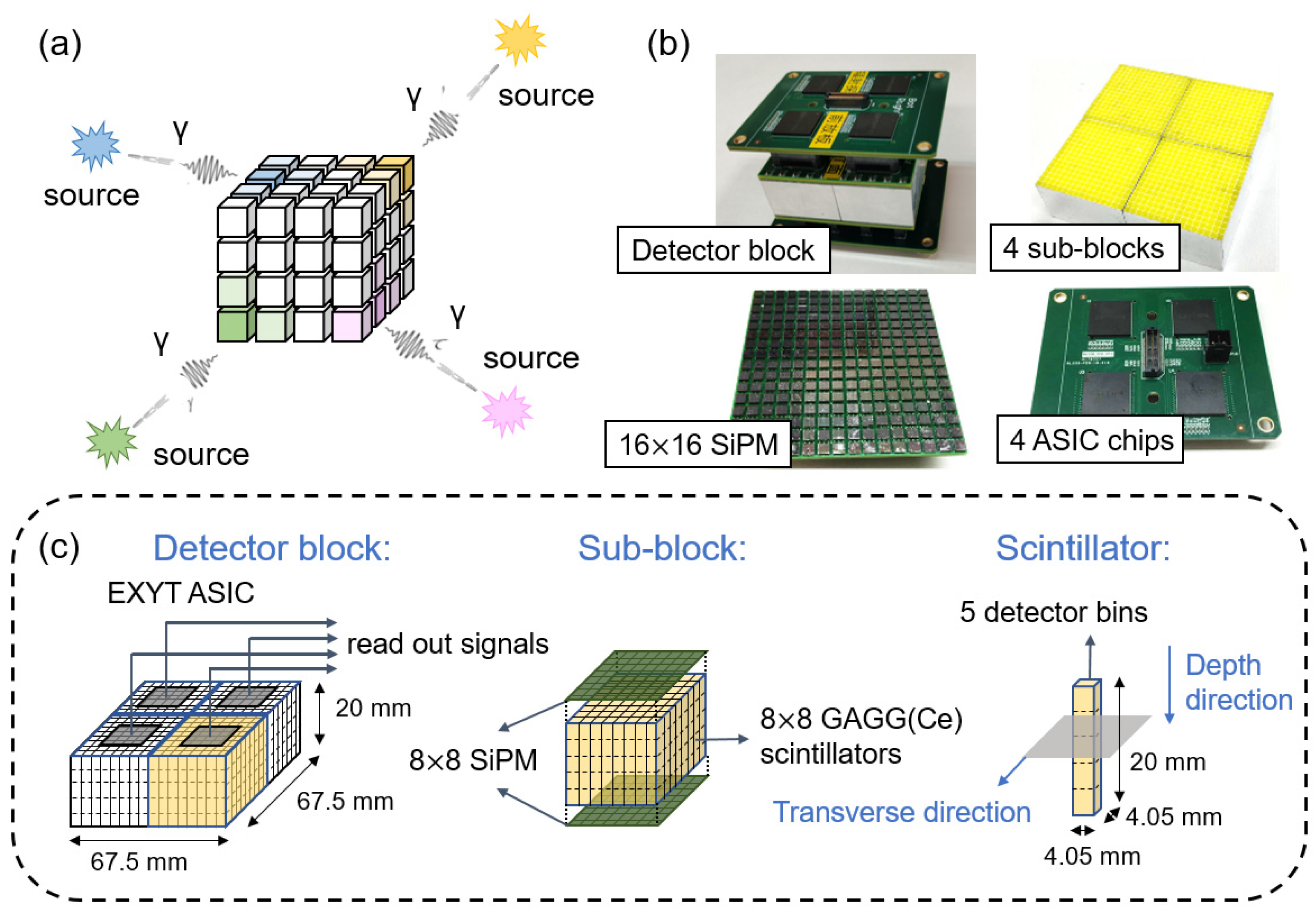
2.1. The 4π-View Gamma Imager

The proposed SM denoising approach is validated with the 4π-view gamma imager developed in our lab. To facilitate understanding, we briefly describe the gamma imager design in this section. Readers are referred to Ref. [26] for more details.

As shown in Figure 1a, the core component of the gamma imager is a 3D position-sensitive radiation detector block. When gamma photons emitted from surrounding radiation source(s) hit the detector block, every detector element has a different photon detection probability depending on the direction of the gamma ray due to varied photon attenuation from other detector elements on the photon path. Therefore, the accumulated photon events’ distribution over a period of time reflects the directional distribution of radiation sources.

As shown in Figure 1b,c, we assembled a realistic detector block with cerium-doped gadolinium aluminum gallium garnet (GAGG(Ce)) scintillator and silicon photomultiplier (SiPM) arrays on both ends. The entire scintillator block was 67.5 × 67.5 × 20 mm³ in size, consisting of 16 × 16 GAGG(Ce) scintillators (EPIC Crystal, Shanghai, China) with a size of 4.05 × 4.05 × 20 mm³. Each scintillator was smeared with a totally reflective material, BaSO₄ (EPIC Crystal, Shanghai, China), on the four side surfaces. Two 16 × 16 SiPM arrays (FJ30035, Onsemi, Phoenix, AZ, USA) were coupled to the dual end surfaces of the scintillator block.

The signals of SiPM arrays were read by a lab-developed ASIC chip [41]. Since each ASIC had 8 × 8 channels, we virtually divided the detector block into 2 × 2 sub-blocks (Figure 1b,c), and each sub-block contained 8 × 8 GAGG(Ce) scintillators. One should note that the sub-block division strategy impacts the detector performance as well as the denoising process (see Section 2.3 and Section 2.4 for details).

To formulate the imaging problem, we defined a spherical coordinate system with the origin at the geometrical center of the detector. As shown in Figure 2, the image was defined on a 4π-view sphere surface, denoted by the polar angle θ and azimuth angle φ. We discretized the image domain into 181(θ) × 360(φ) pixels with a pixel size of 1° × 1°. The radioactivity in the i-th image pixel is denoted as $x_i$.

The detector block measures the 3D position for each detected photon and histograms the measured events into projection {$p_j$}, where $p_j$ denotes the number of photon events in the j-th detector bin. In the transverse direction, the intrinsic detector resolution is determined by the scintillator size; therefore, there are 16 × 16 detector bins transversely. In the depth direction, we use a dual-end read-out technique [27] to calculate the photon interaction position. According to our measurement, the position estimation accuracy is ~4 mm, resulting in 5 detector bins in the depth direction. Therefore, in each scintillator block, we define a total of 16 × 16 × 5 detector bins.

The imaging task aims to reconstruct the radioactivity image $\left\{x_i\right\}$ using the measured projection dataset $\left\{p_j\right\}$. We used the MLEM algorithm [5] in image reconstruction as follows:

$$x_i^{k+1}=\frac{x_i^k}{{\sum }_j{a}_{ij}}{\displaystyle \sum }_j{a}_{ij}\frac{p_j}{{\sum }_i{x}_i^k{a}_{ij}}$$

where $x_i^{k+1}$ and $x_i^k$ indicate the reconstructed images after k + 1 and k iterations, respectively. The system matrix {$a_{ij}$} denotes the probability of one photon emitted from the i-th image voxel and being detected in the j-th detector bin.

2.2. System Matrix Calibration and Detector Response Function

Figure 3a demonstrates a realistic scheme, with multiple gamma imagers manufactured in a volume-producing procedure, that requires extensive SM calibrations. Due to hardware and assembling-induced variations, the SM of each imager needs to be individually calibrated. In this study, we chose two representative imagers, Imager 1 and Imager 2.

In the radiation source monitoring application scenario illustrated in Figure 3b, the gamma imager is installed on the ceiling with a top-view posture. In this case, a 2π image FOV is required. Therefore, although the gamma imager itself allows 4π-imaging, in what follows, we define a 2π-FOV for the realistic imaging system (Figure 3c). The developed methodology is expected to be applicable in the entire 4π-FOV.

In the experimental calibration process, the SM is measured with a point source surrounding the imager and then pre-stored in the computer. Each imager is mounted on a motion controller so that it is rotatable about the center and is exposed to a stationary radioactive source (Figure 3d) to calibrate the system matrix. We rotate the imager to allow hemispherical coverage of the illumination of the point source, which makes θ from 0° to 90° and φ from 0° to 359° (Figure 3c). The whole calibration process is described as follows:

(1)

Define a 10 × 36 grid in the 2π image FOV, with θ ranging from 0° to 90° with 10° intervals and φ ranging from 0° to 350° with 10° intervals.

(2)

Place a point source at the intersection of the grid and measure the projection point by point to generate a coarse-grid SM. The size is 360 (image domain: 10 × 36) × 1280 (projection domain: 16 × 16 × 5).

(3)

Perform spline interpolation to generate a fine-grid SM with a 1° interval. As a result, the size of the fine-grid SM is 32,760 (image domain: 91 × 360) × 1280 (projection domain: 16 × 16 × 5).

The SM of the gamma imager is dependent on the energy of the radiation source. Therefore, the calibration process is repeated for each source. In this study, we chose two representative radiation sources, ^99mTc and ¹³⁷Cs, to investigate the fast calibration approach. The ^99mTc source represents low-energy radiation and is widely used in medical applications. The ¹³⁷Cs source has medium gamma energy and is regularly used in industrial applications.

In a typical calibration process, each of the ^99mTc or ¹³⁷Cs radiation sources used in the calibration has an activity of ~15 mCi and is placed ~0.9 m away from the detector. At each measurement point, we acquire the projection in 15 s durations. The overall calibration measurement requires ~1.4 h for each imager and each radiation source. After spline interpolation, the total number of acquired photon events in each detector bin varies from 1.60 × 10⁶ to 2.17 × 10⁸ for ^99mTc in a 112–168 keV energy window and 5.41 × 10⁶ to 3.59 × 10⁷ for ¹³⁷Cs in a 530–785 keV energy window.

Figure 4a indicates the geometric relationship between the calibration measurement and the measured SM. The projection of each detector bin can be extracted as a column of SM. Figure 4b shows representative columns of the SMs measured in a typical acquisition time (~1.4 h) for two detector bins. There are 360 (φ) × 91 (θ) = 32,760 elements in each column, which is visualized as a 360 × 91 color-scale image. In this work, we define such an image as a detector response function (DRF), as it represents the detection probability distribution for a certain detector bin over all image pixels.

For a single detector bin, gamma photons emitted from different directions have various detection probabilities because of different attenuation distances between sources and the detector bin induced by other detector bins along the path. The total acquired counts in each detector bin and for each radiation source are marked in the upper-right corner of each DRF image in Figure 4b.

In Figure 4c, we show four DRFs that were also acquired for the same detector bins but with a 10% acquisition time. The counts are marked in the upper-right corner. Figure 4d demonstrates line profiles along the white double-headed arrows in Figure 4b,c for DRFs measured in full acquisition time and in 10% acquisition time. Obviously, DRFs measured with a 10% acquisition time differ from their long-time measured counterparts in terms of significantly increased statistical noise. Therefore, an effective denoising process is mandatory for the noisy SM.

In what follows, we chose DRF as the input of neural networks because (1) SM is the combination of DRFs for all the detector bins; thus, denoised SM can be given by assembling all the denoised DRFs together. (2) DRF can be shaped into a 2D smooth image with an appropriate size while retaining the physical meaning, which is beneficial for denoising.

2.3. Self-Adaptive, Sensitivity-Dependent Data-Grouping Strategy

Figure 4b,c shows prominent sensitivity variation (expressed as the sum of values in each DRF image) across different detector bins. In Figure 5a, we show sensitivity maps over the entire detector block for ^99mTc and ¹³⁷Cs sources. The maps are displayed from the side view, and layers 1 to 5 are indicated in the upper row in Figure 5a. Clearly, the sensitivity of each detector bin varies with the position of the detector bin as well as the source type. For the ^99mTc source, the detector bins on the surface have more counts due to the low penetrating capability of the 140 keV gamma ray. The last row of detector bins for each layer has the highest sensitivity due to the lower-hemisphere FOV. Additionally, the discrepancy of properties between each crystal bar and each electronic signal read-out element contributes to the non-uniformity. For the ¹³⁷Cs source, the “cross” pattern is caused by the signal read-out setting described in Section 2.1. Since the signals in each sub-block are read out individually, if a photon interacts with the detector block through Compton scattering and deposits a portion of energy in two sub-blocks, the produced signals on one sub-block or both sub-blocks may be low enough to be rejected by the energy window discrimination logic, leading to a low photon event distribution on the edge of each sub-block. Since it has been shown that the optimal parameter set of a denoising network is highly relevant to the count level of the images [37], the non-uniformity of sensitivity poses a challenge in training denoising networks.

To address this issue, we separated the DRF images into multiple groups according to each detector bin’s sensitivity. For each group, the denoising network training and parameter optimization processes were performed individually.

To accommodate the system response discrepancy for different radioactive sources and different machines, we implemented a self-adaptive, unsupervised K-means clustering algorithm in data grouping. The Euclidean distance was used as a metric of similarity for detector bins’ sensitivity (i.e., the sum of counts in each DRF image). Cluster centroids were initialized with random items, and then DRFs of 1280 detector bins were automatically categorized into three groups according to their sensitivity.

In Figure 5b, we show the total counts in each detector bin in descending order, and the grouping result is labeled with different colors. In both cases of the ^99mTc and ¹³⁷Cs sources, we defined three data groups. For the ^99mTc source, there are 75 DRFs in Group 1 with an average count level of 1.6853 × 10⁸, 167 DRFs in Group 2 with an average count level of 6.9547 × 10⁷, and 1038 DRFs in Group 3 with an average count level of 2.1096 × 10⁷. For the ¹³⁷Cs source, Group 1 has 307 DRFs with 2.4511 × 10⁷ counts on average, Group 2 has 566 DRFs with 1.6439 × 10⁷ counts on average, and Group 3 has 407 DRFs with 1.0682 × 10⁷ counts on average.

We further show the position maps of detectors in each data group (labeled in different colors) for the ^99mTc source and ¹³⁷Cs source in Figure 5c. For each radioactive source and each DRF group, an individual network is trained.

2.4. Deep-Learning-Based Denoising

We proposed two deep learning networks for the SM denoising task: a U-net encoder-decoder network [39] and a residual U-net (Res-U-net) framework, which is the combination of a U-net and a residual connection [42]. Both networks accept DRF images as the network input and produce denoised DRF images as the output.

2.4.1. Network Architectures

U-Net Architecture

Figure 6 illustrates the U-net network architecture in this study. The width of each block indicates the number of feature maps in the layer, the length denotes the input size of the matrix, and the arrows stand for different operations. The entire network consists of an encoder, a bottleneck, and a symmetrical decoder, making up a U-shape. The encoder contains four stacks; in each stack, there are 2 convolutional layers with a 3 × 3 kernel followed by a rectified linear unit (ReLU), and a 2 × 2 max pooling layer with a stride of 2. The bottleneck has 2 convolutional layers. The decoder consists of four stacks of convolutional layers and up-convolutional layers which expand the feature maps. A fully convolutional layer is added to the end to match the feature maps to the label. Between the encoding layers and their corresponding decoding layers, there are skip connections to propagate low-level features to high-resolution layers and compensate for information loss in max pooling.

We created two adaptions from the original U-net [39]. First, image padding was applied in each convolutional layer to keep a constant size of feature maps. Second, since there are 4 max pooling layers and 4 up-convolutional layers, we adapted the length and width of the input image to be multiples of 16 so that the output image had the same size as the input.

Res-U-Net Architecture

Different from the U-net network, in the Res-U-net network structure (as shown in Figure 7), a skip connection is added between the input and output of the whole network. The adoption of the residual connection concept could ease the training of the network, resolve the degradation problem, and potentially improve training accuracy.

2.4.2. Dataset Preparation and Network Training

The training and testing datasets were produced from the SM calibration measurements described in Section 2.2 with the following steps:

(1)

By using all the events acquired in the full acquisition time of Imager 1, we produced a full-count SM (FC-SM).

(2)

We generated low-count SM (LC-SM) by randomly picking 10% events from the fully acquired list mode data, representing an SM that can be measured with a 10% acquisition time.

(3)

We extracted 1280 pairs of full-count DRFs and low-count DRFs from FC-SM and LC-SM and used them as the label and input dataset, respectively, which were fed into the deep networks. For each source energy and each DRF group, an individual network was trained.

(4)

We repeated down-sampling steps (2) and (3) 20 times to produce 20 independent LC-SMs and used all of them as the training data so that the deep networks had sufficient input data to avoid overfitting.

One should note that (1) to match the magnitude of FC-SM, each LC-SM is multiplied by 10, and (2) due to 4 pairs of max pooling and up-convolutional layers in both U-net and Res-U-net architectures, the length and width of input matrix are preferably multiples of 16 to match the size of output figures with that of the input DRFs. Therefore, we added paddings around the input DRFs and transformed their size into 368 × 96.

We ran the network training process separately for each gamma energy and each of the data groups, as described in Section 2.3. All the training data were extracted from the calibration measurements for Imager 1.

We evaluated the efficacy of the trained denoising network with two approaches:

Intra-device testing. We produced another 10 LC-SMs with measured data of Imager 1 as the testing data (statistically independent of the training data). The denoised SMs were compared to the FC-SMs.

Inter-device testing. We produced 1 FC-SM and 10 LC-SMs from the calibrated data of Imager 2. Instead of training other denoising networks for Imager 2, we directly used the network trained with data of Imager 1 to denoise Imager 2′s LC-SMs. We expected this approach to reveal the potential of real-world acceleration of the calibration process in a volume production pipeline since long-time calibration measurement is required for only one device.

However, when implementing inter-device evaluation, the count levels of Imager 1 and Imager 2 were different, even for DRFs from the same detector bin, leading to a mismatch between the training and testing data noise levels. This was caused by the different properties of scintillation crystals and digital processing units from different devices. On the other hand, due to the non-linear response of the networks, the mismatch of the count level should be taken care of. Therefore, we applied detector-by-detector scaling to compensate for the mismatch as follows:

(1)

Calculate DRF-wise scaling factors $\left\{F_j\right\}$, $F_j=\frac{total counts of the j^{th} DRF from Imager1}{total counts of the j^{th} DRF from Imager2}$;

(2)

Generate the input DRFs: $DR{F}_j^{input}=DR{F}_j^{Imager2}\times F_j$;

(3)

Apply the denoising networks on $\{DR{F}_j^{input}\}$ and obtain the outputs $\{DR{F}_j^{output}\}$;

(4)

Implement inverse scaling on the outputs and obtain $\{DR{F}_j^{final}\}$: $DR{F}_j^{final}=DR{F}_j^{output}÷F_j$;

(5)

Re-organize $\{DR{F}_j^{final}\}$ to form a denoised SM of Imager 2.

2.4.3. Implementation Details

We used a batch size of 16 in all the training tasks. The epoch numbers of each network were empirically chosen to assure convergence, as listed in

Table 1. Epoch numbers for training networks.

Epoch Number	U-Net			Res-U-Net
	Group 1	Group 2	Group 3	Group 1	Group 2	Group 3
99mTc	250	225	150	250	200	135
137Cs	125	125	120	120	125	130

. In all the cases, we used the MSE loss function, the Adam optimizer, with an initial learning rate of 0.0001 and an exponential decay rate of 0.996.

All the computations were carried out on a workstation equipped with an NVIDIA GeForce RTX 2080 GPU card. We used a hybrid programming framework with MATLAB V9.8 and Python V3.6 with the PyTorch framework.

2.5. Conventional Gaussian-Filtering-Based Denoise Approach

We also implemented a traditional Gaussian-filtering-based denoising method for comparison. For each individual DRF image, we filtered the image with a 2D Gaussian filtering kernel as follows:

$$G\left(x,y\right)=\frac{1}{2\pi {\sigma }^2}{e}^{-\frac{x^2+y^2}{2{\sigma }^2}}$$

where σ denotes the standard deviation of the Gaussian kernel function. To obtain the best Gaussian filtering performance for fair comparisons, we tested on the LC-SM (Imager 1) data (multiplied by 10 to match the magnitude of FS-SM (Imager 1)) with σ ranging from 0.1 to 15 pixels with a step size of 0.1 pixels for each detector bin. We used a figure-of-merit of the mean square error (MSE) between the full-count DRF image and the filtered low-count DRF image to determine an optimal σ for each DRF. Figure 8 illustrates the MSE curves of two representative detector bins (as indicated in Figure 4a) for ^99mTc and ¹³⁷Cs sources. The optimal σ values that yielded the smallest MSE are marked in each sub-figure.

2.6. Performance Evaluation

2.6.1. SSIM between System Matrices

The structural similarity index (SSIM) directly reflects the difference between FC-SM and the denoised LC-SM. SSIM between two system matrices is represented by the mean SSIM value of each corresponding DRF; additionally, SSIM for each DRF group is calculated by the mean. For two system matrices composed of N DRFs, the formula can be written as follows:

$$SSIM\left(S{M}_1,S{M}_2\right)=\frac{{\sum }_{i=1}^{N}SSIM\left(DR{F}_i\_S{M}_1,DR{F}_i\_S{M}_2\right)}{N}$$

2.6.2. Positioning Bias

We tested the positioning accuracy by imaging a single point source at exactly known angular positions. We experimentally placed a point source at 6 × 6 different positions with θ = {17°, 35°, 46°, 53°, 64°, 81°} and φ = {64°, 82°, 127°, 189°, 261°, 333°}. The distribution map of testing positions is shown in Figure 9. At each point, we collected around 1M photon events. Each reconstructed image was calculated with 10,000 MLEM iterations. The experiments were conducted twice, one with a ^99mTc source and the other with a ¹³⁷Cs source.

We calculated the positioning bias, which refers to the deviation between the reconstructed position of the radioactive source and the ground truth (denoted as ${\theta }_{true}$ and ${\phi }_{true}$). The reconstructed position $\widehat{\theta }$ and $\widehat{\phi }$ is determined by the centroid of the image in both θ and φ directions:

$$\widehat{\theta }=\frac{{\sum }_{\theta }{\sum }_{\phi }\theta \times v\left(\theta ,\phi \right)}{{\sum }_{\theta }{\sum }_{\phi }v\left(\theta ,\phi \right)}$$

$$\widehat{\phi }=\frac{{\sum }_{\phi }{\sum }_{\theta }\phi \times v\left(\theta ,\phi \right)}{{\sum }_{\phi }{\sum }_{\theta }v\left(\theta ,\phi \right)}$$

where $v\left(\theta ,\phi \right)$ represents the value at pixel location $\left(\theta ,\phi \right)$ of the reconstructed image. Then, positioning bias was calculated by:

$$bias=\arccos \left(\frac{\overrightarrow{\left(\widehat{\theta },\widehat{\phi }\right)}·\overrightarrow{\left({\theta }_{true},{\phi }_{true}\right)}}{\left|\overrightarrow{\left(\widehat{\theta },\widehat{\phi }\right)}\right|\times \left|\overrightarrow{\left({\theta }_{true},{\phi }_{true}\right)}\right|}\right)$$

2.6.3. FWHM Resolution

Image resolution is also an important image quality index. We calculated the full-width-half-maximum (FWHM) resolution from the reconstructed single-point-source images described in Section 2.6.2. We fit each image with a 2D non-isotropic Gaussian function, from which we calculated the FWHM of the point source in both θ and φ directions. Then, we calculated the FWHM resolution as

$$resolution=\sqrt{{\left(FWH{M}_{\theta }\right)}^2+{\left(FWH{M}_{\phi }\right)}^2}$$

3. Results

3.1. Intra-Device Evaluation

3.1.1. Denoised SMs

We chose 10 LC-SMs of Imager 1 as the testing set to perform intra-device evaluation. Figure 10 and Figure 11 show representative DRF images of FC-SM, LC-SM, Gaussian-filtering-based denoised SM (G-DSM), U-net-based denoised SM (U-DSM), and Res-U-net-based denoised SM (R-DSM) for ^99mTc and ¹³⁷Cs sources, respectively. We also statistically calculated the SSIM value between each DRF image and the corresponding FC-SM case, shown in the bottom-right corners of the images. For each group, we chose one representative detector bin (indicated in the first row in Figure 10 and Figure 11 with a highlighted box) and plotted its DRFs in the rest of the rows.

For both the ^99mTc source and ¹³⁷Cs source, the DRFs of LC-SMs (third row in Figure 10 and Figure 11) are evidently different from those of FC-SMs (second row) due to increased noise. Compared with LC-SMs, the DRFs of G-DSMs (fourth row) are much smoother after Gaussian filtering but with an unavoidable loss of details. DRFs of U-DSMs (fifth row) and those of R-DSMs (sixth row) are visually more similar to those of FC-SMs after U-net-based denoising and Res-U-net-based denoising, respectively. R-DSMs yield slightly better recovery of details.

The mean and standard deviation (SD) of SSIM calculated for 10 testing LC-SMs and FC-SM, as well as those between DSMs and FC-SM for ^99mTc and ¹³⁷Cs sources, are listed in

Table 2. SSIM (mean ± SD) with FC-SM of LC-SMs, G-DSMs, U-DSMs, and R-DSMs for ^99mTc.

SM	LC-SM	G-DSM	U-DSM	R-DSM
SSIM	0.6484 ± 0.0005	0.7433 ± 0.0004	0.8490 ± 0.0005	0.8542 ± 0.0004

and

Table 3. SSIM (mean ± SD) with FC-SM of LC-SMs, G-DSMs, U-DSMs, and R-DSMs for ¹³⁷Cs.

SM	LC-SM	G-DSM	U-DSM	R-DSM
SSIM	0.5208 ± 0.0005	0.6146 ± 0.0004	0.8641 ± 0.0007	0.8542 ± 0.0004

, respectively. For both ^99mTc and ¹³⁷Cs sources, the three denoising methods can improve SSIM, among which U-DSMs and R-DSMs reach higher SSIM values, while G-DSMs have the worst performance.

3.1.2. Performance of Reconstructed Images—Positioning Bias

In terms of image reconstruction evaluation, we tested the 36 different point source positions described in Section 2.6.2. The projections used for reconstruction were also measured in experiments with a count level of 1M. Each reconstructed image was obtained using the MLEM algorithm with 10,000 iterations.

The reconstructed images of ^99mTc and ¹³⁷Cs point sources at five representative positions are illustrated in Figure 12 and Figure 13, respectively. The yellow box and green cross in each of the images in the first column indicate the zone for displaying the zoomed images and the true position of the point source. One can observe in Figure 12 and Figure 13 that the image quality of LC-SM is poor with dispersive hot-dot artifacts. Using Gaussian-filtered SMs moderately improves the image quality; however, in certain positions, there are still visible artifacts, which lead to notable positioning bias. After implementing U-net-based denoising and Res-U-net-based denoising, the reconstructed images were obviously more similar to those with FC-SM, leading to better positional accuracy.

In Figure 14 and Figure 15, we present box plots for the mean value and SD of the positioning bias of reconstructed images at the 36 different source positions indicated in Figure 9. We first calculated the mean value and SD for the 10 testing datasets at each source position for LC-SM, G-DSM, U-DSM, and R-DSM cases. Then, the mean and SD results at all 36 source positions were presented in box plots. It is important to note that since there is only one dataset for FC-SM, the mean positioning bias is exactly the value of the single dataset, and there is no SD statistics result for FC-SM. Both U-net and Res-U-net-based denoising achieve <2.5° positioning bias for ^99mTc source and <2° for ¹³⁷Cs source, outperforming LC-SM and G-DSM. Additionally, U-DSM and R-DSM have a lower bias SD, indicating that the deep-learning-based denoising methods are more robust for different LC-SMs than Gaussian filtering. In Figure 15b, the bias SD of U-DSM concentrates around 0.2°, making the box plot a line.

3.1.3. Image Performance—FWHM Resolution

The mean and SD values of FWHM resolution for ^99mTc and ¹³⁷Cs at 36 different source positions are shown in Figure 16 and Figure 17, respectively. For the ^99mTc source, the mean resolution for FC-SM, U-DSM, and R-DSM mostly stayed below 20°, better than LC-SM and G-DSM. For the ¹³⁷Cs source, both U-net- and Res-U-net-based deep learning methods achieved around 10~20° image resolution with a few exceptions, outperforming the 20~45° resolution with LC-SM and 10~35° with G-DSM. The SD values of U-DSM and R-DSM were also much lower for both ^99mTc and ¹³⁷Cs sources, indicating that the SMs with deep learning denoising methods yield more robust image reconstruction.

3.2. Inter-Device Evaluation

3.2.1. Imaging Performance—Positioning Bias

As described in Section 2.4.2, for inter-device evaluation, we trained the denoising networks with data measured in Imager 1 and applied the networks in the denoising tasks for Imager 2. Figure 18 and Figure 19 show the reconstructed images of ^99mTc and ¹³⁷Cs point sources at five representative positions. The images in the second to sixth columns correspond to the reconstructed images using an FC-SM, an LC-SM, and three denoised SMs with the Gaussian filtering method (G-DSM), with the U-net-based denoising method (U-DSM), and with the Res-U-net based denoising method (R-DSM). One can observe severe distortion with a noisy LC-SM (third column) or G-DSM (fourth column). U-DSM and R-DSM (fifth and sixth columns) yield better image quality and visually more similar image shapes to the FC-SM cases (second columns).

Quantitative analyses of the mean and SD values of positioning bias are summarized in Figure 20 and Figure 21 for the two radiation sources. For the ^99mTc source, the positioning bias is <2.6° in all cases. Although the image quality of LC-SM has an evident degradation, as shown in Figure 18, the positioning bias does not significantly increase, probably due to the centroid calculation step. In general, LC-SM, G-DSM, U-DSM, and R-DSM show comparable positioning accuracy, among which U-DSM performs slightly poorer. However, as shown in Figure 20b, the SD values of positioning bias for U-DSM and R-DSM are significantly smaller than those for other cases. For the ¹³⁷Cs source (Figure 21a), U-DSM and R-DSM achieve <2.5° average positioning bias, close to that of FC-SM. For LC-SM and G-DSM cases, the mean positioning bias is higher, ranging up to 5°. In Figure 21b, the SD values of the positioning bias for U-DSM and R-DSM cases outperform those for LC-SM and G-DSM cases.

3.2.2. Imaging Performance—FWHM Resolution

The FWHM resolution performance analyses are summarized in Figure 22 and Figure 23 for ^99mTc and ¹³⁷Cs sources, respectively. Figure 22a and Figure 23a clearly reveal that with U-DSM and R-DSM, the mean values of image resolution are obviously better than the LC-SM and G-DSM cases and are close to the FC-SM case. The SD values of resolution (as shown in Figure 22b and Figure 23b) also demonstrate the advantage of deep-learning-based denoising over LC-SM and G-DSM cases. There are no significant differences between the imaging performance using U-net and Res-U-net networks.

4. Discussion

In this study, we proposed a deep-learning-based denoising method to realize time-efficient SM calibration for a 4π-view gamma detector. Two network architectures were investigated, including U-net and Res-U-net, and they both outperformed the non-denoised LC-SM and the denoised SM with conventional Gaussian filtering method in terms of more accurate source position estimation and improved FWHM resolution. The trained networks were validated with the measured data both from the same imager device as well as a different imager to test the versatility of the proposed method. With our proposed method, the system matrix calibration time can be significantly reduced from 1.4 h to 8 min while positioning accuracy and image resolution remain comparable.

To accommodate the significant response discrepancy between different detector elements, we proposed a self-adaptive data-grouping method and trained a separate network for each group. We clustered the DRF images into three different groups to accommodate different noise levels. The number of groups was chosen as a balance among various considerations, e.g., count distribution determined by signal read-out setup, image FOV, and attenuation features of gamma photons in GAGG(Ce). Using more groups might further reduce the discrepancy but at the cost of data processing complexity. Having fewer DRF images in one group may also reduce the training capacity for each network and cause over-fitting. However, the data-grouping strategy can be flexible for different system designs.

The convergence property and model performance varied among different DRF groups. Taking ^99mTc as an example, Figure 24 and Figure 25 show the training loss of three different groups for the U-net model and Res-U-net model, respectively. For both networks, Group 1 takes the largest number of epochs to converge, and Group 3 takes the fewest. This is because Group 1 comprises the fewest DRF images; thus, there are fewer iterations in one epoch, and Group 3 has more iterations in one epoch. In

Table 4. SSIM (mean ± SD) of different DRF groups for LC-SM, G-DSM, U-DSM, and R-DSM for ^99mTc.

SSIM	LC-SM	G-DSM	U-DSM	R-DSM
Group 1	0.8984 ± 0.0010	0.9450 ± 0.0008	0.9861 ± 0.0002	0.9928 ± 0.0002
Group 2	0.7766 ± 0.0008	0.8267 ± 0.0007	0.9261 ± 0.0006	0.9400 ± 0.0008
Group 3	0.6097 ± 0.0006	0.7153 ± 0.0006	0.8267 ± 0.0006	0.8303 ± 0.0005

, we list the mean and SD of SSIM of different DRF groups calculated between 10 testing LC-SMs and FC-SM as well as those between DSMs and FC-SM for ^99mTc. For all the cases, SSIM decreases from Group 1 to Group 3. We believe this is because the detector bins in Group 1 have higher sensitivity and lower noise; therefore, they are more similar to the full-count case. In general, the deep-learning-based denoising approach can improve the SSIM of all three DRF groups and outperforms Gaussian filtering.

The imaging performance of ^99mTc and ¹³⁷Cs sources is different. One can notice in Figure 12, Figure 13, Figure 18 and Figure 19 that the image quality of ^99mTc is intrinsically better than that of ¹³⁷Cs, with fewer dispersive artifacts. Additionally, the image degradation of ¹³⁷Cs is also much more severe than ^99mTc, referring to positioning accuracy as well as resolution. We believe that is because the higher-energy gamma photons of ¹³⁷Cs (662 keV) have stronger penetration capability through the detector, which reduces the sensitivity and increases the noise. On the other hand, increased Compton scattering interactions for the ¹³⁷Cs source may also lead to image degradation. However, compared with ^99mTc, the proposed deep-learning-based denoising methods have more significant improvements for ¹³⁷Cs. We believe this is because the adverse impacts of LC-SM are stronger for ¹³⁷Cs than for ^99mTc, especially when focusing on positioning bias.

There are other ways to further optimize our work. First, the performance of deep learning is highly dependent on the extensiveness of training data, so it would be better to use data generated from more devices to train the networks. In the present study, we only used the SM data from one device (Imager 1) for training. Additionally, when performing an inter-device evaluation, the mismatch of noise levels caused by different hardware leads to performance degradation compared to intra-device evaluation. In future work, we will utilize SM data from different devices for network training to improve reliability. Second, in this study, we selected two radioactive isotopes, ^99mTc and ¹³⁷Cs, as representatives of the most regularly used gamma sources in medical and industrial applications. We planned to test the method with expanded collections of gamma sources in further implementations. Third, in this study, we mainly focused on applying deep learning denoising on the system matrix and practically resolving the problem of the gamma imager calibration process. Therefore, we utilized classical network architectures to primarily prove the feasibility of the approach. The hyperparameters of the networks were chosen referring to existing works which have achieved satisfactory results [35,39]. However, more comprehensive optimization of the network parameters may further improve the performance. In future work, we plan to conduct an ablation study on the network parameters (e.g., number of convolutional layers, kernel size, optimizer) for better results and explore other deep-learning models (e.g., generative adversarial network (GAN) [43]) for the SM denoising task. Additionally, the extension of datasets mentioned above may also help improve the model’s efficiency.

Our proposed deep-learning-based denoising method generally applies to other imaging systems that rely on an experimental calibration step to accommodate comprehensive system response factors in an accurately measured SM. Our proposed method effectively addresses the challenge of long calibration time, which represents a major obstruction that limits the application of experimental measurement in real practice. We expect that the presented technique can be extended to other gamma imaging devices, including industrial gamma cameras, SPECT, and PET systems.

5. Conclusions

In this study, we proposed a time-efficient SM calibration method with short-time measured SM and deep-learning-based denoising. To deal with sensitivity discrepancy across different detector bins, we proposed a self-adaptive, K-means clustering method to classify DRF images into multiple groups fed to independent network training processes. We investigated two denoising networks with U-net and Res-U-net architectures and compared them against a conventional Gaussian filtering method. Through intra-device and inter-device studies, we demonstrated that the denoised SMs with deep networks effectively reduce the noise-induced image degradation and faithfully yield comparable imaging performance with the long-time measured SM. Henceforth, the system matrix calibration time can be reduced from 1.4 h to 8 min. We conclude that the proposed SM denoising approach is promising and effective in enhancing the productivity of the 4π-view gamma imager, and it is also generally applicable to other imaging systems that require an experimental calibration step.

References

1. Fenimore, E.E.; Cannon, T.M. Coded aperture imaging with uniformly redundant arrays. Appl. Opt. 1978, 17, 337–347. [Google Scholar] [CrossRef] [PubMed]
2. Cieślak, M.J.; Gamage, K.A.A.; Glover, R. Coded-aperture imaging systems: Past, present and future development—A review. Radiat. Meas. 2016, 92, 59–71. [Google Scholar] [CrossRef]
3. Kishimoto, A.; Kataoka, J.; Nishiyama, T.; Taya, T.; Kabuki, S. Demonstration of three-dimensional imaging based on handheld Compton camera. J. Instrum. 2015, 10, P11001. [Google Scholar] [CrossRef]
4. Liu, Y.; Fu, J.; Li, Y.; Li, Y.; Ma, X.; Zhang, L. Preliminary results of a Compton camera based on a single 3D position-sensitive CZT detector. Nucl. Sci. Tech. 2018, 29, 145. [Google Scholar] [CrossRef]
5. Lange, K.; Carson, R. EM Reconstruction Algorithms for Emission and Transmission Tomography. J. Comput. Assist. Tomogr. 1984, 8, 306–316. [Google Scholar]
6. Sengee, N.; Radnaabazar, C.; Batsuuri, S.; Tsedendamba, K.O. A Comparison of Filtered Back Projection and Maximum Likelihood Expected Maximization. In Proceedings of the 2017 International Conference on Computational Biology and Bioinformatics—ICCBB 2017, Newark, NJ, USA, 18–20 October 2017; pp. 68–73. [Google Scholar]
7. Gottesman, S.R.; Fenimore, E.E. New family of binary arrays for coded aperture imaging. Appl. Opt. 1989, 28, 4344–4352. [Google Scholar] [CrossRef]
8. Rahmim, A.; Qi, J.; Sossi, V. Resolution modeling in PET imaging: Theory, practice, benefits, and pitfalls. Med. Phys. 2013, 40, 64301. [Google Scholar] [CrossRef] [Green Version]
9. Presotto, L.; Gianolli, L.; Gilardi, M.C.; Bettinardi, V. Evaluation of image reconstruction algorithms encompassing Time-Of-Flight and Point Spread Function modelling for quantitative cardiac PET: Phantom studies. J. Nucl. Cardiol. 2015, 22, 351–363. [Google Scholar] [CrossRef]
10. Laurette, I.; Zeng, G.L.; Welch, A.; Christian, P.E.; Gullberg, G.T. A three-dimensional ray-driven attenuation, scatter and geometric response correction technique for SPECT in inhomogeneous media. Phys. Med. Biol. 2000, 45, 3459. [Google Scholar] [CrossRef]
11. Rafecas, M.; Boning, G.; Pichler, B.J.; Lorenz, E.; Schwaiger, M.; Ziegler, S.I. Effect of Noise in the Probability Matrix Used for Statistical Reconstruction of PET Data. IEEE Trans. Nucl. Sci. 2004, 51, 149–156. [Google Scholar] [CrossRef]
12. Metzler, S.D.; Bowsher, J.E.; Greer, K.L.; Jaszczak, R.J. Analytic determination of the pinhole collimator’s point-spread function and RMS resolution with penetration. IEEE Trans. Med. Imaging 2002, 21, 878–887. [Google Scholar] [CrossRef] [PubMed]
13. Bequé, D.; Nuyts, J.; Bormans, G.; Suetens, P.; Dupont, P. Characterization of pinhole SPECT acquisition geometry. IEEE Trans. Med. Imaging 2003, 22, 599–612. [Google Scholar] [CrossRef] [PubMed]
14. Accorsi, R.; Metzler, S.D. Analytic determination of the resolution-equivalent effective diameter of a pinhole collimator. IEEE Trans. Med. Imaging 2004, 23, 750–763. [Google Scholar] [CrossRef] [PubMed]
15. Nguyen, M.P.; Goorden, M.C.; Ramakers, R.M.; Beekman, F.J. Efficient Monte-Carlo based system modelling for image reconstruction in preclinical pinhole SPECT. Phys. Med. Biol. 2021, 66, 125013. [Google Scholar] [CrossRef] [PubMed]
16. Auer, B.; Zeraatkar, N.; Banerjee, S.; Goding, J.C.; Furenlid, L.R.; King, M.A. Preliminary investigation of a Monte Carlo-based system matrix approach for quantitative clinical brain 123I SPECT imaging. In Proceedings of the 2018 IEEE Nuclear Science Symposium and Medical Imaging Conference Proceedings (NSS/MIC), Sydney, NSW, Australia, 10–17 November 2018; pp. 1–2. [Google Scholar]
17. Rafecas, M.; Mosler, B.; Dietz, M.; Pögl, M.; Stamatakis, A.; McElroy, D.P.; Ziegler, S.I. Use of a monte carlo-based probability matrix for 3-D iterative reconstruction of MADPET-II data. IEEE Trans. Nucl. Sci. 2004, 51, 2597–2605. [Google Scholar] [CrossRef]
18. Rowe, R.K.; Aarsvold, J.N.; Barrett, H.H.; Chen, J.-C.; Klein, W.P.; Moore, B.A.; Pang, I.W.; Patton, D.D.; White, T.A. A Stationary Hemispherical SPECT Imager for Three-Dimensional Brain Imaging. J. Nucl. Med. 1993, 34, 474. [Google Scholar]
19. Furenlid, L.R.; Wilson, D.W.; Chen, Y.C.; Kim, H.; Pietraski, P.J.; Crawford, M.J.; Barrett, H.H. FastSPECT II: A Second-Generation High-Resolution Dynamic SPECT Imager. IEEE Trans. Nucl. Sci. 2004, 51, 631–635. [Google Scholar] [CrossRef]
20. Van der Have, F.; Vastenhouw, B.; Rentmeester, M.; Beekman, F.J. System calibration and statistical image reconstruction for ultra-high resolution stationary pinhole SPECT. IEEE Trans. Med. Imaging 2008, 27, 960–971. [Google Scholar] [CrossRef] [Green Version]
21. Miller, B.W.; Van Holen, R.; Barrett, H.H.; Furenlid, L.R. A System Calibration and Fast Iterative Reconstruction Method for Next-Generation SPECT Imagers. IEEE Trans. Nucl. Sci. 2012, 59, 1990–1996. [Google Scholar] [CrossRef] [Green Version]
22. Hu, Y.; Fan, P.; Lyu, Z.; Huang, J.; Wang, S.; Xia, Y.; Liu, Y.; Ma, T. Design and performance evaluation of a 4π-view gamma camera with mosaic-patterned 3D position-sensitive scintillators. Nucl. Instrum. Methods Phys. Res. Sect. A Accel. Spectrometers Detect. Assoc. Equip. 2022, 1023, 165971. [Google Scholar] [CrossRef]
23. Murata, T.; Miwa, K.; Miyaji, N.; Wagatsuma, K.; Hasegawa, T.; Oda, K.; Umeda, T.; Iimori, T.; Masuda, Y.; Terauchi, T.; et al. Evaluation of spatial dependence of point spread function-based PET reconstruction using a traceable point-like (22)Na source. EJNMMI Phys. 2016, 3, 26. [Google Scholar] [CrossRef] [PubMed] [Green Version]
24. Liu, Y.; Xiao, X.; Zhang, Z.; Wei, L. Near-field artifacts reduction in coded aperture push-broom Compton scatter imaging. Nucl. Instrum. Methods Phys. Res. Sect. A Accel. Spectrometers Detect. Assoc. Equip. 2020, 957, 163385. [Google Scholar] [CrossRef]
25. Nuyts, J.; Vunckx, K.; Defrise, M.; Vanhove, C. Small animal imaging with multi-pinhole SPECT. Methods 2009, 48, 83–91. [Google Scholar] [CrossRef] [PubMed]
26. Ye, Q.; Fan, P.; Wang, R.; Lyu, Z.; Hu, A.; Wei, Q.; Xia, Y.; Yao, R.; Liu, Y.; Ma, T. A high sensitivity 4π view gamma imager with a monolithic 3D position-sensitive detector. Nucl. Instrum. Methods Phys. Res. Sect. A Accel. Spectrometers Detect. Assoc. Equip. 2019, 937, 31–40. [Google Scholar] [CrossRef]
27. Fan, P.; Xu, T.; Lyu, Z.; Wang, S.; Liu, Y.; Ma, T. 3D positioning and readout channel number compression methods for monolithic PET detector. In Proceedings of the 2016 IEEE Nuclear Science Symposium, Medical Imaging Conference and Room-Temperature Semiconductor Detector Workshop (NSS/MIC/RTSD), Strasbourg, France, 29 October–6 November 2016; pp. 1–4. [Google Scholar]
28. Lyu, Z.; Fan, P.; Liu, Y.; Wang, S.; Wu, Z.; Ma, T. Timing Estimation Algorithm Incorporating Spatial Position for Monolithic PET Detector. In Proceedings of the 2017 IEEE Nuclear Science Symposium and Medical Imaging Conference (NSS/MIC), Atlanta, GA, USA, 21–28 October 2017; pp. 1–3. [Google Scholar]
29. Lyu, Z.; Fan, P.; Xu, T.; Wang, R.; Liu, Y.; Wang, S.; Wu, Z.; Ma, T. Improved Spatial Resolution and Resolution Uniformity of Monolithic PET Detector by Optimization of Photon detector Arrangement. In Proceedings of the 2017 IEEE Nuclear Science Symposium and Medical Imaging Conference (NSS/MIC), Atlanta, GA, USA, 21–28 October 2017; pp. 1–4. [Google Scholar]
30. Deng, G.; Cahill, L.W. An adaptive Gaussian filter for noise reduction and edge detection. In Proceedings of the 1993 IEEE Conference Record Nuclear Science Symposium and Medical Imaging Conference, San Francisco, CA, USA, 31 October–6 November 1993; Volume 1613, pp. 1615–1619. [Google Scholar]
31. Buades, A.; Coll, B.; Morel, J. A non-local algorithm for image denoising. In Proceedings of the 2005 IEEE Computer Society Conference on Computer Vision and Pattern Recognition (CVPR’05), San Diego, CA, USA, 20–25 June 2005; Volume 62, pp. 60–65. [Google Scholar]
32. Dougherty, E.R.; Dabov, K.; Astola, J.T.; Foi, A.; Katkovnik, V.; Egiazarian, K.O.; Nasrabadi, N.M.; Egiazarian, K.; Rizvi, S.A. Image denoising with block-matching and 3D filtering. In Proceedings of the Image Processing: Algorithms and Systems, Neural Networks, and Machine Learning, San Jose, CA, USA, 16–18 January 2006. [Google Scholar]
33. Lu, S.; Tan, J.; Gao, Y.; Shi, Y.; Liang, Z.; Bosmans, H.; Chen, G.-H. Prior knowledge driven machine learning approach for PET sinogram data denoising. In Proceedings of the Medical Imaging 2020: Physics of Medical Imaging, Houston, TX, USA, 16–19 February 2020. [Google Scholar]
34. Ma, Y.; Ren, Y.; Feng, P.; He, P.; Guo, X.; Wei, B. Sinogram denoising via attention residual dense convolutional neural network for low-dose computed tomography. Nucl. Sci. Tech. 2021, 32, 1–14. [Google Scholar] [CrossRef]
35. Lu, W.; Onofrey, J.A.; Lu, Y.; Shi, L.; Ma, T.; Liu, Y.; Liu, C. An investigation of quantitative accuracy for deep learning based denoising in oncological PET. Phys. Med. Biol. 2019, 64, 165019. [Google Scholar] [CrossRef] [PubMed]
36. Geng, M.; Meng, X.; Yu, J.; Zhu, L.; Jin, L.; Jiang, Z.; Qiu, B.; Li, H.; Kong, H.; Yuan, J.; et al. Content-Noise Complementary Learning for Medical Image Denoising. IEEE Trans. Med. Imaging 2022, 41, 407–419. [Google Scholar] [CrossRef]
37. Gong, K.; Guan, J.; Kim, K.; Zhang, X.; Yang, J.; Seo, Y.; Fakhri, E.G.; Qi, J.; Li, Q. Iterative PET Image Reconstruction Using Convolutional Neural Network Representation. IEEE Trans. Med. Imaging 2019, 38, 675–685. [Google Scholar] [CrossRef]
38. Haggstrom, I.; Schmidtlein, C.R.; Campanella, G.; Fuchs, T.J. DeepPET: A deep encoder-decoder network for directly solving the PET image reconstruction inverse problem. Med. Image Anal. 2019, 54, 253–262. [Google Scholar] [CrossRef]
39. Ronneberger, O.; Fischer, P.; Brox, T. U-Net: Convolutional Networks for Biomedical Image Segmentation. In Proceedings of the Medical Image Computing and Computer-Assisted Intervention—MICCAI 2015, Munich, Germany, 5–9 October 2015; pp. 234–241. [Google Scholar]
40. Tripathi, M. Facial image denoising using AutoEncoder and UNET. Herit. Sustain. Dev. 2021, 3, 89–96. [Google Scholar] [CrossRef]
41. Zhu, X.; Deng, Z.; Chen, Y.; Liu, Y.; Liu, Y. Development of a 64-Channel Readout ASIC for an SSPM Array for PET and TOF-PET Applications. IEEE Trans. Nucl. Sci. 2016, 63, 1–8. [Google Scholar] [CrossRef]
42. He, K.; Zhang, X.; Ren, S.; Sun, J. Deep residual learning for image recognition. In Proceedings of the IEEE Conference on Computer Vision and Pattern Recognition, Las Vegas, NV, USA, 27–30 June 2016; pp. 770–778. [Google Scholar]
43. Goodfellow, I.; Pouget-Abadie, J.; Mirza, M.; Xu, B.; Warde-Farley, D.; Ozair, S.; Courville, A.; Bengio, Y. Generative Adversarial Nets. In Proceedings of the Neural Information Processing Systems, Montréal, QC, Canada, 8–13 December 2014. [Google Scholar]
Figure 1. (a) Illustration of imaging concept of 3D position-sensitive detector block. (b) Pictures of detector block prototype. (c) Illustration of the detector block design.
Sensors 23 02689 g001
Figure 2. Illustration of the geometrical setup of the imaging problem.
Sensors 23 02689 g002
Figure 3. (a) Picture of several gamma imagers. (b) Illustration of radiation source monitoring scenario. (c) Illustration of system matrix calibration setup. (d) Picture of realistic system matrix calibration process.
Sensors 23 02689 g003
Figure 4. (a) Illustration of the geometrical relationship between calibration measurement (left) and the measured SM (right). (b) DRF images of two representative detector bins for 99mTc and 137Cs sources (measured with the full acquisition time). (c) DRF images of two representative detector bins for 99mTc and 137Cs sources (measured with a 10% acquisition time). (d) Line profiles of DRF images measured with the full acquisition time (with scale marked on the left) and 10% acquisition time (with scale marked on the right).
Sensors 23 02689 g004
Figure 5. (a) Sensitivity maps of detector bins for 99mTc and 137Cs sources. (b) Histogram of total counts of DRFs for each detector bin and grouping results for 99mTc and 137Cs sources. (c) The position maps of detectors in each data group for 99mTc and 137Cs sources.
Sensors 23 02689 g005
Figure 6. Architecture of the U-net network.
Sensors 23 02689 g006
Figure 7. Architecture of the Res-U-net network.
Sensors 23 02689 g007
Figure 8. σ-MSE curves of representative detector bins for 99mTc and 137Cs sources.
Sensors 23 02689 g008
Figure 9. Distribution map of 36 different testing positions.
Sensors 23 02689 g009
Figure 10. Representative DRF images of FC-SM, LC-SM, G-DSM, U-DSM, and R-DSM for 99mTc source. SSIM value between each DRF image and FC-SM case is given in the bottom-right corner.
Sensors 23 02689 g010
Figure 11. Representative DRF images of FC-SM, LC-SM, G-DSM, U-DSM, and R-DSM for 137Cs source. SSIM value between each DRF image and FC-SM case is given in the bottom-right corner.
Sensors 23 02689 g011
Figure 12. Reconstructed images of different SMs at representative positions for 99mTc source in intra-device evaluation.
Sensors 23 02689 g012
Figure 13. Reconstructed images of different SMs at representative positions for 137Cs source in intra-device evaluation.
Sensors 23 02689 g013
Figure 14. Box plots of (a) mean values and (b) SD values of positioning bias at 36 different source positions for 99mTc source in intra-device evaluation.
Sensors 23 02689 g014
Figure 15. Box plots of (a) mean values and (b) SD values of positioning bias at 36 different source positions for 137Cs source in intra-device evaluation.
Sensors 23 02689 g015
Figure 16. Box plots of (a) mean values and (b) SD values of FWHM resolution at 36 different source positions for 99mTc source in intra-device evaluation.
Sensors 23 02689 g016
Figure 17. Box plots of (a) mean values and (b) SD values of FWHM resolution at 36 different source positions for 137Cs source in intra-device evaluation.
Sensors 23 02689 g017
Figure 18. Reconstructed images of different SMs at representative positions for 99mTc source in inter-device evaluation.
Sensors 23 02689 g018
Figure 19. Reconstructed images of different SMs at representative positions for 137Cs source in inter-device evaluation.
Sensors 23 02689 g019
Figure 20. Box plots of (a) mean values and (b) SD values of positioning bias at 36 different source positions for 99mTc source in inter-device evaluation.
Sensors 23 02689 g020
Figure 21. Box plots of (a) mean values and (b) SD values of positioning bias at 36 different source positions for 137Cs source in inter-device evaluation.
Sensors 23 02689 g021
Figure 22. Box plots of (a) mean values and (b) SD values of FWHM resolution at 36 different source positions for 99mTc source in inter-device evaluation.
Sensors 23 02689 g022
Figure 23. Box plots of (a) mean values and (b) SD values of FWHM resolution at 36 different source positions for 137Cs source in inter-device evaluation.
Sensors 23 02689 g023
Figure 24. Training loss of different DRF groups with U-net model for 99mTc.
Sensors 23 02689 g024
Figure 25. Training loss of different DRF groups with Res-U-net model for 99mTc.
Sensors 23 02689 g025