
ConnecSenS, a Versatile IoT Platform for Environment Monitoring: Bring Water to Cloud
 , , , and
Abstract
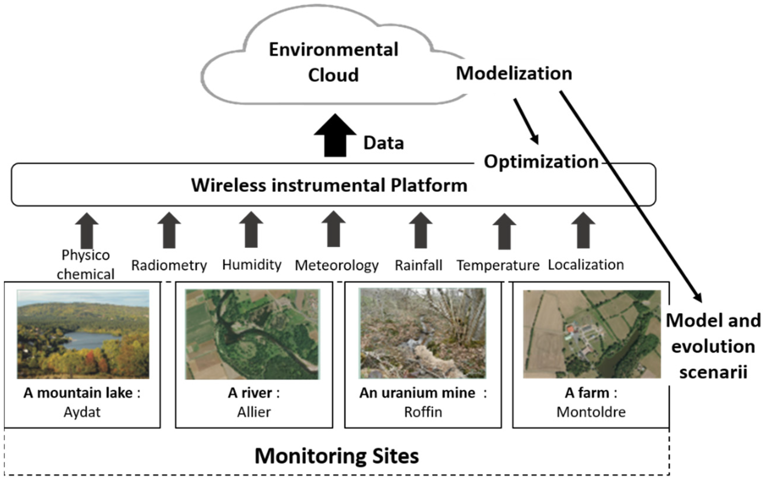
:1. Introduction
2. Materials and Methods
2.1. Private LoraWAN Network
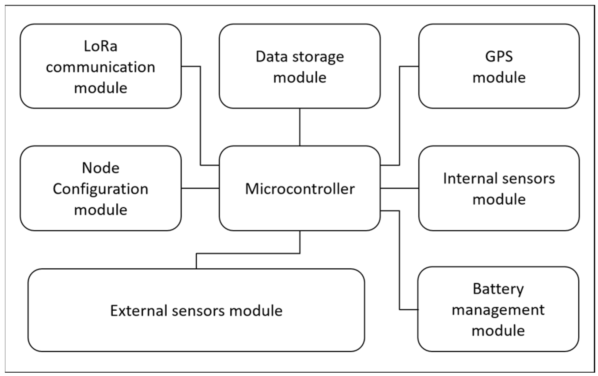
2.2. Node SoLo (Sensors Open Lora Node)
2.2.1. General Presentation of the Node
2.2.2. Firmware Presentation
2.3. Data Workflow
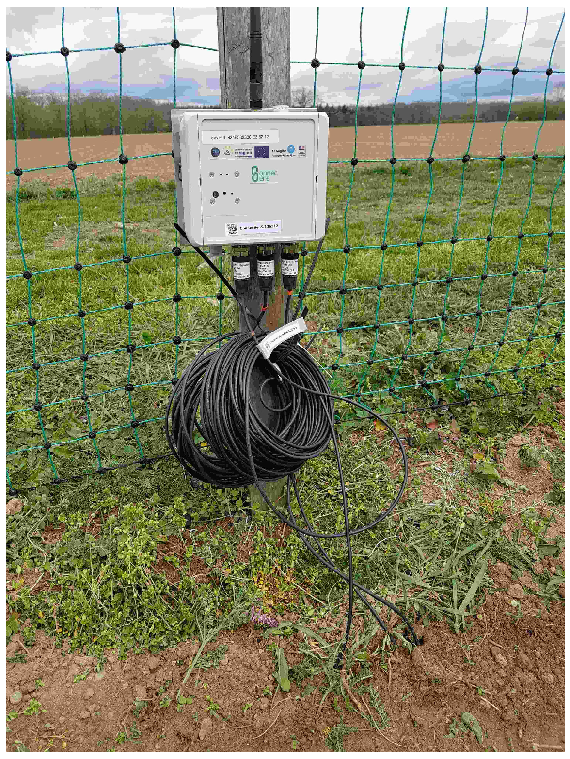
2.4. Monitoring Sites
- The Aydat site is a mountain lake subject to the impacts of agricultural practices and recurrent cyanobacterial proliferation;
- The Allier River site is a river channel connected to an oxbow lake whose hydroecological responses to climate change must be understood;
- The Roffin site is a former uranium mine that can have a long-term impact on a watercourse and its vegetation;
- The Montoldre site is a farm where water is an input to be optimized.
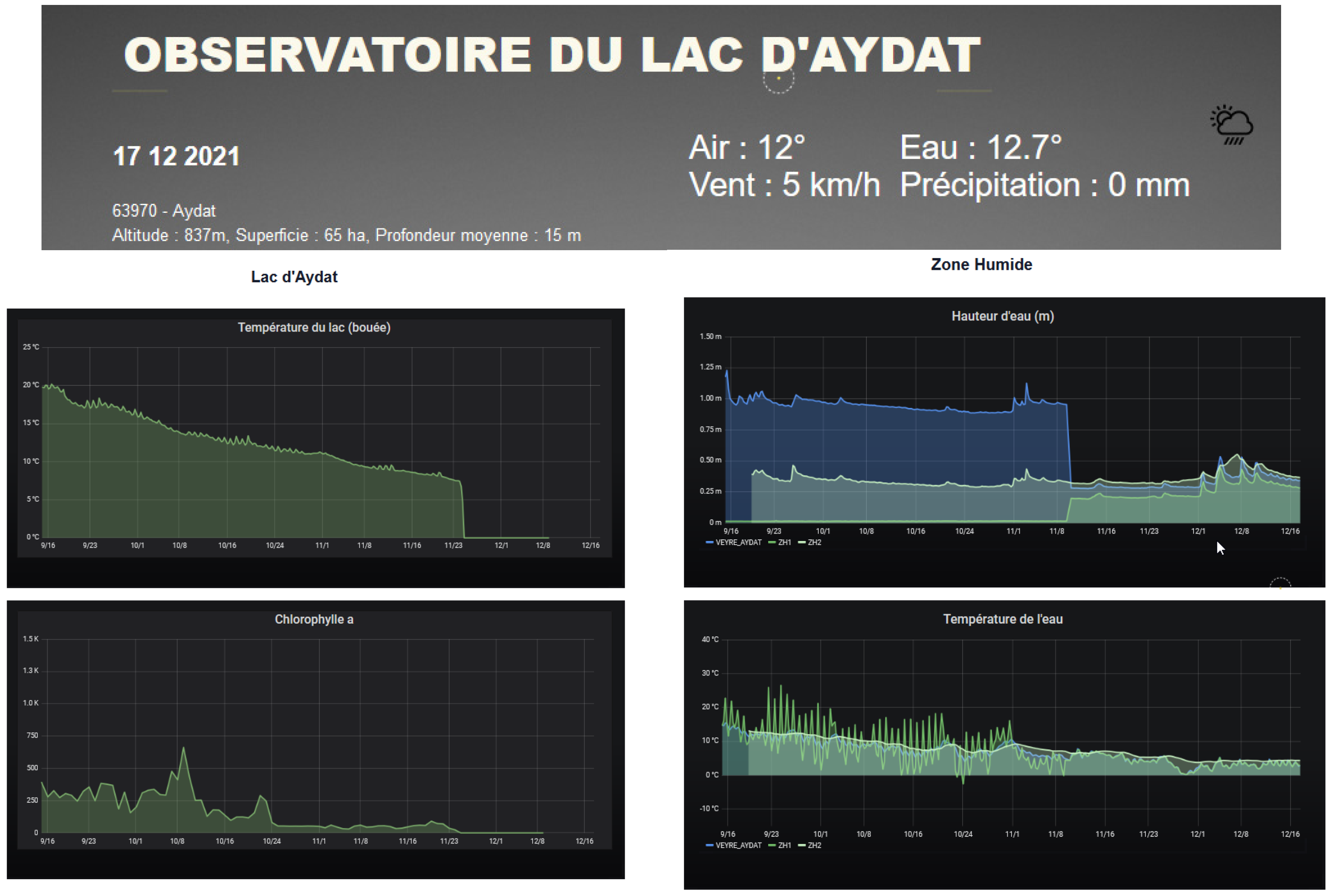
2.4.1. Aydat Lake
- Site description
- Scientific objectives
- Sensors
- 1–3: Aquatroll 200 data logger. This water level and water temperature probe is installed in the Veyre river, upstream and downstream of the lake. The water level measurement is based on a piezoresistive sensor, whereas the water temperature and the specific conductivity, the salinity, and the Total Dissolved Solids (TDS) are monitored using a balanced 4-electrode cell. The water discharge series can be computed using a rating curve calibrated with a gauging protocol.
- 4: Hydrolab HL7 multiparameter sonde. The multiparameter sonde comprises eight sensors, including an electrical conductivity sensor, a Hach LDO® Dissolved Oxygen Sensor, a temperature sensor, a turbidity sensor, chlorophyll-a sensor, a blue and green algae sensor, rhodamine sensor, and finally a pressure sensor for water depth measurement. The Hach LDO® Dissolved Oxygen Sensor provides a measure with Luminescent Dissolved Oxygen (LDO) technology. The Hydrolab conductivity sensor uses four graphite electrodes in an open-cell design to provide highly accurate and reliable data. The sensor measures specific conductance, salinity, total dissolved solids (TDS), and resistivity. The conductivity sensor uses four graphite electrodes designed to be compliant with the ISO 7027 Turbidity Measurement Standard. The Hydrolab temperature sensor is a variable resistance thermistor (316 stainless steel for corrosion resistance). Hydrolab sondes are available with integrated pressure sensors that provide depth measurements. Data acquisition of each parameter takes place every hour.
- 5: Temperature data logger. The HOBO data loggers record temperature with the high-frequency acquisition (i.e., 5 min), located in the middle point of the Aydat lake, every 20 cm from the water surface to 3 m deep. The upstream river temperature (Veyre) is also monitored with eight HOBO data loggers regularly distributed (every 1 km) from the headwater to the river mouth.
2.4.2. Allier River
- Site description
- Scientific objectives
- Sensors
2.4.3. Roffin Mine
- Site description
- Scientific objectives
- Sensors
2.4.4. Montoldre Farm
- Site description
- Scientific objectives
3. Results and Discussion
3.1. Real-Time Visualization of the Data
3.2. Data Analysis
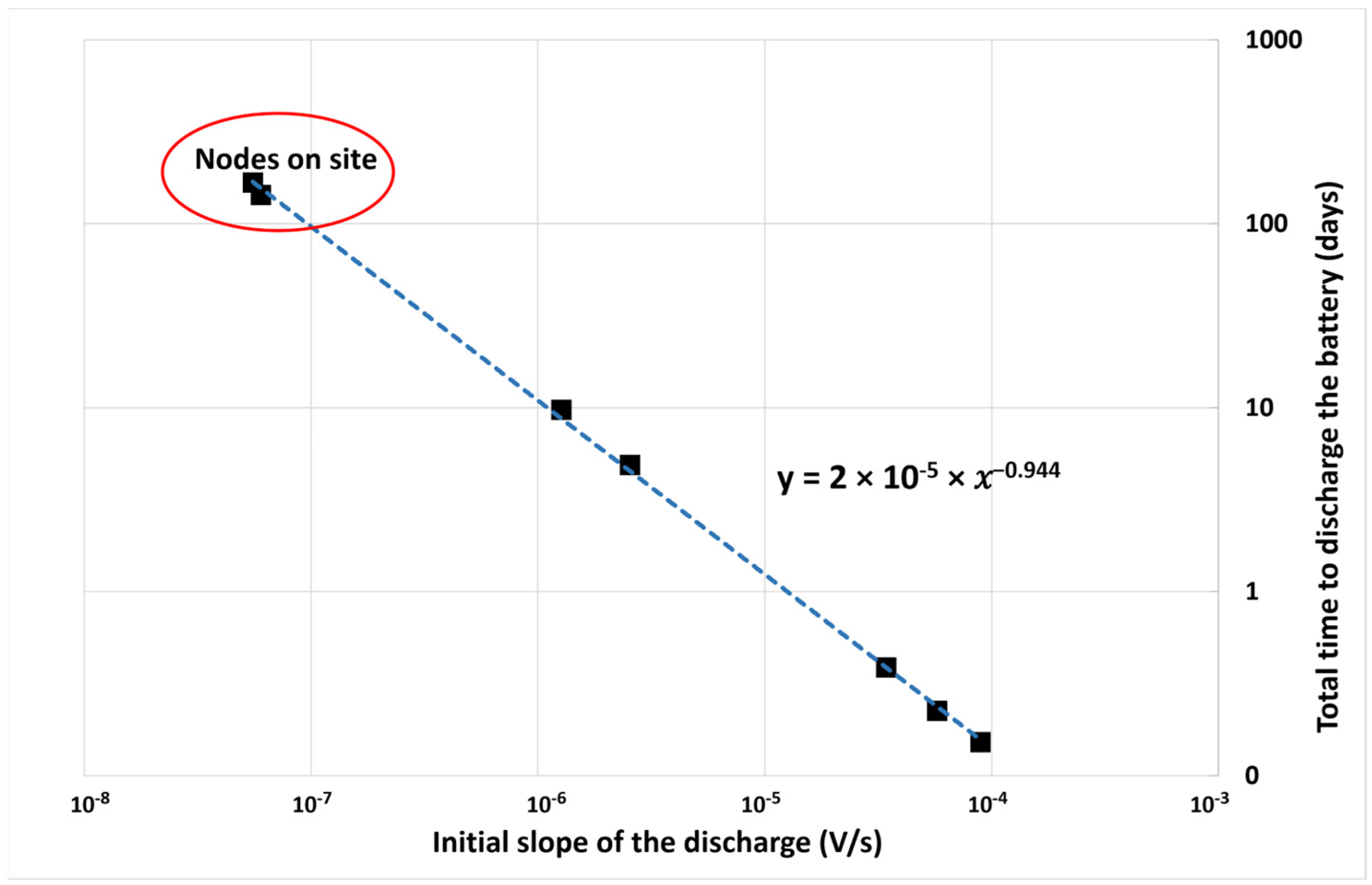
3.2.1. Battery Lifetime Estimation
- The power consumption of the LoRa radio transceiver depends on the modulation parameters. Therefore, the channel frequency is set to 868 MHz, the bandwidth to 125 kHz, and the transmission power fixed to 25 mW. However, the spreading factor (7 to 12) can be selected through the data rate (5 to 0) parameter inside the configuration file;
- The power consumption of the internal sensors which the operator has activated;
- The power consumption of external sensors if the node itself provides the power;
- The period of data acquisition;
- The period of data transmission;
- The temperature of the battery cells has a significant impact on their discharge capacity (70% at 0 °C, 40% at −10 °C).
3.2.2. Packet Loss Analysis
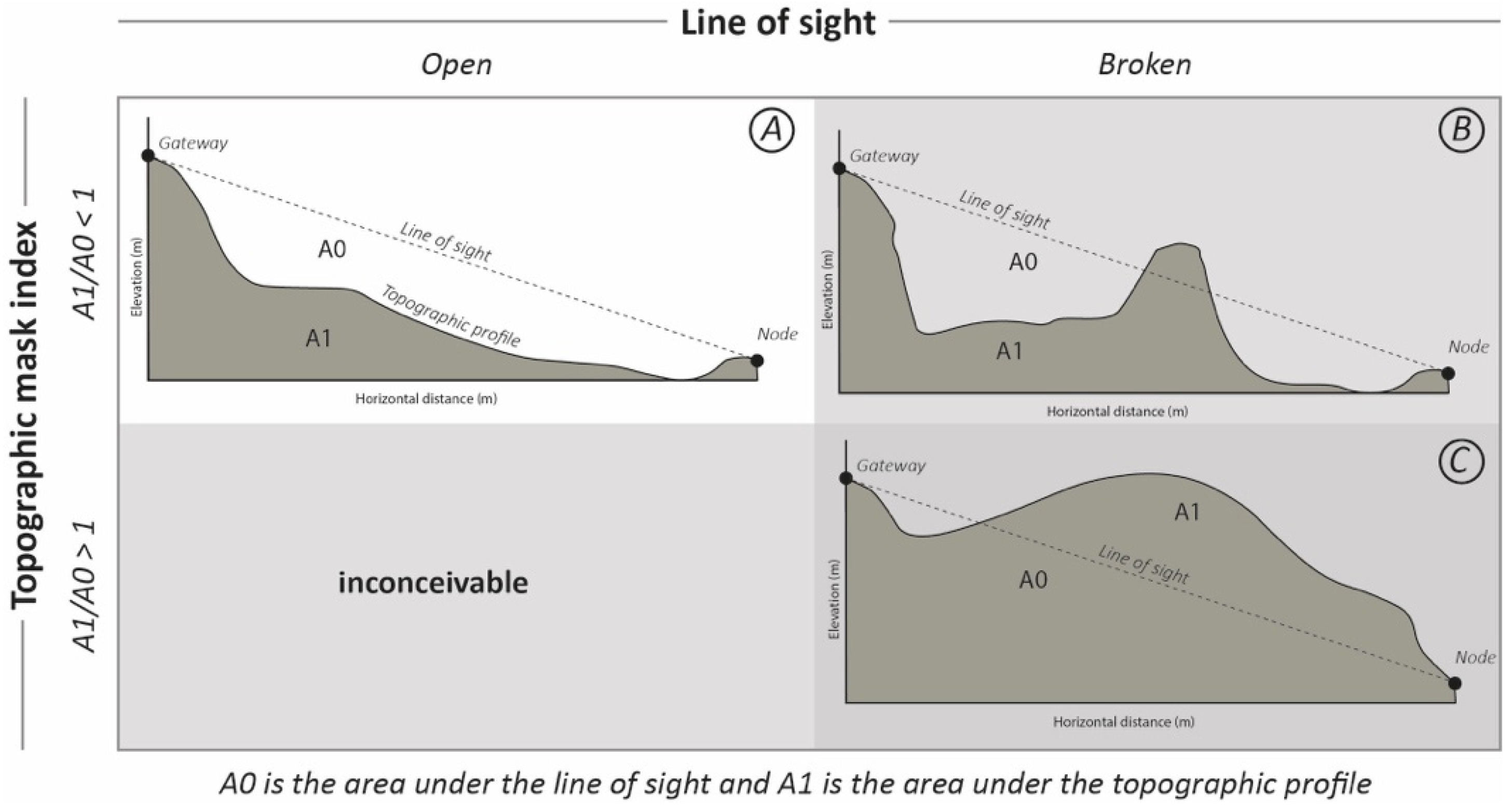
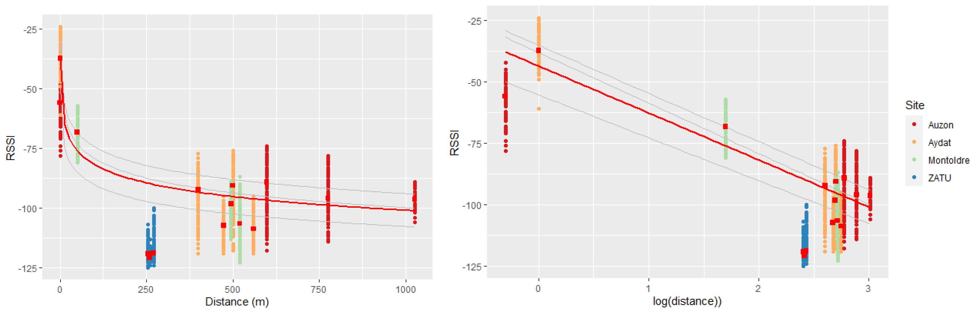
3.2.3. Analysis of LoRa Signal Strengths Attenuation as a Function of Distance and Visibility Parameters (Path-Loss Model)
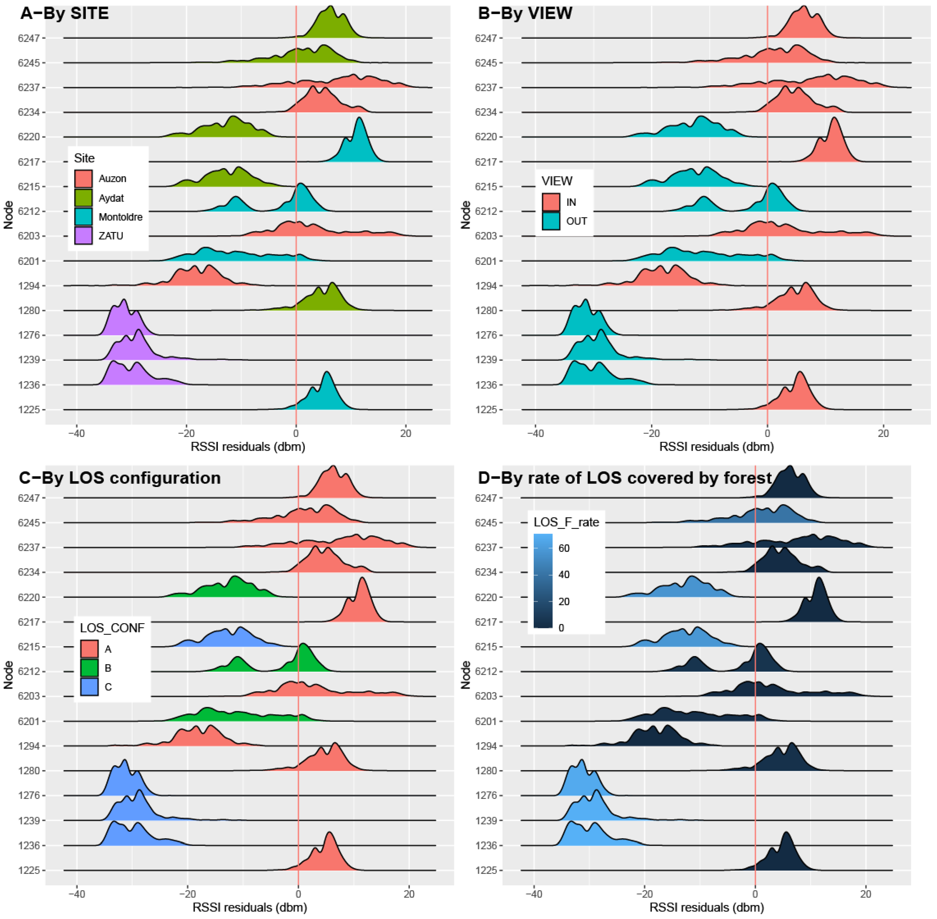
3.2.4. RSSI Variation with the Geographical Distance to the Gateways
4. Conclusions
5. Patents
Author Contributions
Funding
Acknowledgments
Conflicts of Interest
References
- Whitehead, P.G.; Wilby, R.L.; Batterbee, R.W.; Kernan, M.; Wade, A.J. A Review of the Potential Impacts of Climate Change on Surface Water Quality. Hydrol. Sci. J. 2009, 54, 101–123. [Google Scholar] [CrossRef] [Green Version]
- Piao, S.; Ciais, P.; Huang, Y.; Shen, Z.; Peng, S.; Li, J.; Zhou, L.; Liu, H.; Ma, Y.; Ding, Y.; et al. The Impacts of Climate Change on Water Resources and Agriculture in China. Nature 2010, 467, 43–51. [Google Scholar] [CrossRef] [PubMed]
- Mukheibir, P. Water Access, Water Scarcity, and Climate Change. Environ. Manag. 2010, 45, 1027–1039. [Google Scholar] [CrossRef] [PubMed] [Green Version]
- Oliveira, L.M.; Rodrigues, J.J. Wireless Sensor Networks: A Survey on Environmental Monitoring. J. Commun. 2011, 6, 143–151. [Google Scholar] [CrossRef] [Green Version]
- Othman, M.F.; Shazali, K. Wireless Sensor Network Applications: A Study in Environment Monitoring System. Procedia Eng. 2012, 41, 1204–1210. [Google Scholar] [CrossRef] [Green Version]
- Ullo, S.L.; Sinha, G.R. Advances in Smart Environment Monitoring Systems Using IoT and Sensors. Sensors 2020, 20, 3113. [Google Scholar] [CrossRef]
- Kamienski, C.; Soininen, J.-P.; Taumberger, M.; Dantas, R.; Toscano, A.; Cinotti, T.S.; Maia, R.F.; Neto, A.T. Smart Water Management Platform: IoT-Based Precision Irrigation for Agriculture. Sensors 2019, 19, 276. [Google Scholar] [CrossRef] [Green Version]
- Mazumdar, S.; Seybold, D.; Kritikos, K.; Verginadis, Y. A Survey on Data Storage and Placement Methodologies for Cloud-Big Data Ecosystem. J. Big Data 2019, 6, 15. [Google Scholar] [CrossRef] [Green Version]
- Mansouri, Y.; Toosi, A.N.; Buyya, R. Data Storage Management in Cloud Environments: Taxonomy, Survey, and Future Directions. ACM Comput. Surv. 2017, 50, 91:1–91:51. [Google Scholar] [CrossRef]
- Hartung, C.; Han, R.; Seielstad, C.; Holbrook, S. FireWxNet: A Multi-Tiered Portable Wireless System for Monitoring Weather Conditions in Wildland Fire Environments. In Proceedings of the 4th international Conference on Mobile Systems, Applications and Services, Uppsala, Sweden, 19–22 June 2006; Association for Computing Machinery: New York, NY, USA, 2006; pp. 28–41. [Google Scholar]
- Fang, S.; Xu, L.D.; Zhu, Y.; Ahati, J.; Pei, H.; Yan, J.; Liu, Z. An Integrated System for Regional Environmental Monitoring and Management Based on Internet of Things. IEEE Trans. Ind. Inform. 2014, 10, 1596–1605. [Google Scholar] [CrossRef]
- Benghanem, M. Measurement of Meteorological Data Based on Wireless Data Acquisition System Monitoring. Appl. Energy 2009, 86, 2651–2660. [Google Scholar] [CrossRef]
- Gulati, K.; Kumar Boddu, R.S.; Kapila, D.; Bangare, S.L.; Chandnani, N.; Saravanan, G. A Review Paper on Wireless Sensor Network Techniques in Internet of Things (IoT). Mater. Today Proc. 2022, 51, 161–165. [Google Scholar] [CrossRef]
- Yetgin, H.; Cheung, K.T.K.; El-Hajjar, M.; Hanzo, L.H. A Survey of Network Lifetime Maximization Techniques in Wireless Sensor Networks. IEEE Commun. Surv. Tutor. 2017, 19, 828–854. [Google Scholar] [CrossRef] [Green Version]
- Saini, H.; Thakur, A.; Ahuja, S.; Sabharwal, N.; Kumar, N. Arduino Based Automatic Wireless Weather Station with Remote Graphical Application and Alerts. In Proceedings of the 2016 3rd International Conference on Signal Processing and Integrated Networks (SPIN), Noida, India, 11–12 February 2016; pp. 605–609. [Google Scholar]
- Faludi, R. Building Wireless Sensor Networks: With ZigBee, XBee, Arduino, and Processing; O’Reilly Media, Inc.: Sebastopol, CA, USA, 2010; ISBN 978-1-4493-0274-0. [Google Scholar]
- Ferdoush, S.; Li, X. Wireless Sensor Network System Design Using Raspberry Pi and Arduino for Environmental Monitoring Applications. Procedia Comput. Sci. 2014, 34, 103–110. [Google Scholar] [CrossRef] [Green Version]
- Widhalm, D.; Goeschka, K.M.; Kastner, W. Is Arduino a Suitable Platform for Sensor Nodes? In Proceedings of the IECON 2021—47th Annual Conference of the IEEE Industrial Electronics Society, Toronto, ON, Canada, 13–16 October 2021; pp. 1–6. [Google Scholar]
- Kondaveeti, H.K.; Kumaravelu, N.K.; Vanambathina, S.D.; Mathe, S.E.; Vappangi, S. A Systematic Literature Review on Prototyping with Arduino: Applications, Challenges, Advantages, and Limitations. Comput. Sci. Rev. 2021, 40, 100364. [Google Scholar] [CrossRef]
- Kone, C.T.; Mathias, J.-D.; Sousa, G.D. Adaptive Management of Energy Consumption, Reliability and Delay of Wireless Sensor Node: Application to IEEE 802.15.4 Wireless Sensor Node. PLoS ONE 2017, 12, e0172336. [Google Scholar] [CrossRef] [Green Version]
- Bhola, J.; Shabaz, M.; Dhiman, G.; Vimal, S.; Subbulakshmi, P.; Soni, S.K. Performance Evaluation of Multilayer Clustering Network Using Distributed Energy Efficient Clustering with Enhanced Threshold Protocol. Wirel. Pers. Commun. 2022, 126, 2175–2189. [Google Scholar] [CrossRef]
- Lilhore, U.K.; Khalaf, O.I.; Simaiya, S.; Romero, C.A.T.; Abdulsahib, G.M.; Poongodi, M.; Kumar, D. A Depth-Controlled and Energy-Efficient Routing Protocol for Underwater Wireless Sensor Networks. Int. J. Distrib. Sens. Netw. 2022, 18, 15501329221117118. [Google Scholar] [CrossRef]
- Vidhya, V.; Madheswaran, M. Data Compression and Transmission Techniques in Wireless Adhoc Networks: A Review. In Intelligent Computing and Networking; Balas, V.E., Semwal, V.B., Khandare, A., Eds.; Springer Nature: Singapore, 2022; pp. 194–206. [Google Scholar]
- Abdalkafor, A.S.; Aliesawi, S.A. Data Aggregation Techniques in Wireless Sensors Networks (WSNs): Taxonomy and an Accurate Literature Survey. AIP Conf. Proc. 2022, 2400, 020012. [Google Scholar] [CrossRef]
- El-Sayed, W.M.; El-Bakry, H.M.; El-Sayed, S.M. Integrated Data Reduction Model in Wireless Sensor Networks. Appl. Comput. Inform. 2020, 19, 41–63. [Google Scholar] [CrossRef]
- William, P.; Badholia, A.; Verma, V.; Sharma, A.; Verma, A. Analysis of Data Aggregation and Clustering Protocol in Wireless Sensor Networks Using Machine Learning. In Evolutionary Computing and Mobile Sustainable Networks; Suma, V., Fernando, X., Du, K.-L., Wang, H., Eds.; Springer: Singapore, 2022; pp. 925–939. [Google Scholar]
- Yakine, F.; Kenzi, A. Energy Harvesting in Wireless Communication: A Survey. E3S Web Conf. 2022, 336, 00074. [Google Scholar] [CrossRef]
- Lafforgue, M.; Szeligiewicz, W.; Devaux, J.; Poulint, M. Selective Mechanisms Controlling Algal Succession in Aydat Lake. Water Sci. Technol. 1995, 32, 117–127. [Google Scholar] [CrossRef]
- Beauger, A.; Lair, N.; Reyes-Marchant, P.; Peiry, J.-L. The Distribution of Macroinvertebrate Assemblages in a Reach of the River Allier (France), in Relation to Riverbed Characteristics. Hydrobiologia 2006, 571, 63–76. [Google Scholar] [CrossRef]
- National Inventory of Uranium Mining Sites. Version 1. Made in the Framework of the Mimausa Program (Memory and Impact of Uranium Mines, Synthesis and Archives); Inventaire National des Sites Miniers D’uranium. Version 1. Realise Dans le Cadre du Programme Mimausa (Memoire et Impact des Mines D’uranium: Synthese et Archives). 2004. Available online: https://www.osti.gov/etdeweb/biblio/20666401 (accessed on 20 December 2022).
- Haxhibeqiri, J.; De Poorter, E.; Moerman, I.; Hoebeke, J. A Survey of LoRaWAN for IoT: From Technology to Application. Sensors 2018, 18, 3995. [Google Scholar] [CrossRef] [PubMed] [Green Version]
- Gaitan, N.C. A Long-Distance Communication Architecture for Medical Devices Based on LoRaWAN Protocol. Electronics 2021, 10, 940. [Google Scholar] [CrossRef]
- Almuhaya, M.A.M.; Jabbar, W.A.; Sulaiman, N.; Abdulmalek, S. A Survey on LoRaWAN Technology: Recent Trends, Opportunities, Simulation Tools and Future Directions. Electronics 2022, 11, 164. [Google Scholar] [CrossRef]
- Miles, B.; Bourennane, E.-B.; Boucherkha, S.; Chikhi, S. A Study of LoRaWAN Protocol Performance for IoT Applications in Smart Agriculture. Comput. Commun. 2020, 164, 148–157. [Google Scholar] [CrossRef]
- ST STM32 Arm Cortex MCUs—32-Bit Microcontrollers—STMicroelectronics. Available online: https://www.st.com/en/microcontrollers-microprocessors/stm32-32-bit-arm-cortex-mcus.html (accessed on 1 December 2021).
- De Carvalho Silva, J.; Rodrigues, J.J.P.C.; Alberti, A.M.; Solic, P.; Aquino, A.L.L. LoRaWAN—A Low Power WAN Protocol for Internet of Things: A Review and Opportunities. In Proceedings of the 2nd International Multidisciplinary Conference on Computer and Energy Science (SpliTech 2017), Split, Croatia, 12–14 July 2017; pp. 1–6. [Google Scholar]
- Erturk, M.A.; Aydin, M.A.; Buyukakkaslar, M.T.; Evirgen, H. A Survey on LoRaWAN Architecture, Protocol and Technologies. Future Internet 2019, 11, 216. [Google Scholar] [CrossRef] [Green Version]
- ChirpStack ChirpStack Open-Source LoRaWAN® Network Server. Available online: https://www.chirpstack.io/ (accessed on 20 December 2022).
- The Things Network The Things Stack. Available online: https://www.thethingsindustries.com/docs/ (accessed on 20 December 2022).
- Grafana Dashboard Anything. Observe Everything. Available online: https://grafana.com/grafana/ (accessed on 20 December 2022).
- Kibana Your Window into the Elastic Stack. Available online: https://www.elastic.co/kibana/ (accessed on 20 December 2022).
- MQTT MQTT: The Standard for IoT Messaging. Available online: https://mqtt.org/ (accessed on 20 December 2022).
- Elactic Suite ELK : Elasticsearch, Logstash et Kibana. Available online: https://www.elastic.co/fr/what-is/elk-stack (accessed on 1 December 2021).
- Sarramia, D.; Claude, A.; Ogereau, F.; Mezhoud, J.; Mailhot, G. CEBA: A Data Lake for Data Sharing and Environmental Monitoring. Sensors 2022, 22, 2733. [Google Scholar] [CrossRef]
- Wen, J.; Dargie, W. Characterization of Link Quality Fluctuation in Mobile Wireless Sensor Networks. ACM Trans. Cyber-Phys. Syst. 2021, 5, 28:1–28:24. [Google Scholar] [CrossRef]
- Liu, W.; Xia, Y.; Zheng, D.; Xie, J.; Luo, R.; Hu, S. Environmental Impacts on Hardware-Based Link Quality Estimators in Wireless Sensor Networks. Sensors 2020, 20, 5327. [Google Scholar] [CrossRef]
- Dillon, K.P.; Correa, F.; Judon, C.; Sancelme, M.; Fennell, D.E.; Delort, A.-M.; Amato, P. Cyanobacteria and Algae in Clouds and Rain in the Area of Puy de Dôme, Central France. Appl. Environ. Microbiol. 2020, 87, e01850-20. [Google Scholar] [CrossRef]
- Hilborn, E.D.; Beasley, V.R. One Health and Cyanobacteria in Freshwater Systems: Animal Illnesses and Deaths Are Sentinel Events for Human Health Risks. Toxins 2015, 7, 1374–1395. [Google Scholar] [CrossRef] [Green Version]
- Masters, B. The Ability of Vegetated Floating Islands to Improve Water Quality in Natural and Constructed Wetlands: A Review. Water Pract. Technol. 2012, 7, wpt2012022. [Google Scholar] [CrossRef]
- Garófano-Gómez, V.; Metz, M.; Egger, G.; Díaz-Redondo, M.; Hortobágyi, B.; Geerling, G.; Corenblit, D.; Steiger, J. Vegetation Succession Processes and Fluvial Dynamics of a Mobile Temperate Riparian Ecosystem: The Lower Allier River (France). Géomorphologie Relief Process. Environ. 2017, 23, 187–202. [Google Scholar] [CrossRef] [Green Version]
- Beauger, A.; Delcoigne, A.; Voldoire, O.; Serieyssol, K.; Peiry, J.-L. Distribution of Diatom, Macrophyte and Benthic Macroinvertebrate Communities Related to Spatial and Environmental Characteristics: The Example of a Cut-Off Meander of the River Allier (France). Cryptogam. Algol. 2015, 36, 323–355. [Google Scholar] [CrossRef]
- Quenet, M.; Celle-Jeanton, H.; Voldoire, O.; Albaric, J.; Huneau, F.; Peiry, J.-L.; Allain, E.; Garreau, A.; Beauger, A. Coupling Hydrodynamic, Geochemical and Isotopic Approaches to Evaluate Oxbow Connection Degree to the Main Stream and to Adjunct Alluvial Aquifer. J. Hydrol. 2019, 577, 123936. [Google Scholar] [CrossRef]
- Van Looy, K.; Piffady, J. Metapopulation Modelling of Riparian Tree Species Persistence in River Networks under Climate Change. J. Environ. Manag. 2017, 202, 437–446. [Google Scholar] [CrossRef]
- Giuntoli, I.; Renard, B.; Vidal, J.-P.; Bard, A. Low Flows in France and Their Relationship to Large-Scale Climate Indices. J. Hydrol. 2013, 482, 105–118. [Google Scholar] [CrossRef] [Green Version]
- Chauveau, M.; Chazot, S.; Perrin, C.; Bourgin, P.-Y.; Sauquet, E.; Vidal, J.-P.; Rouchy, N.; Martin, E.; David, J.; Norotte, T.; et al. Quels Impacts Des Changements Climatiques Sur Les Eaux de Surface En France à l’horizon 2070? Houille Blanche 2013, 99, 5–15. [Google Scholar] [CrossRef] [Green Version]
- Moatar, F.; Ducharne, A.; Thiéry, D.; Bustillo, V.; Sauquet, E.; Vidal, J.-P. La Loire à l’épreuve Du Changement Climatique. Géosciences 2010, 12, 78–87. [Google Scholar]
- Ameglio, T.; Dusotoit-Coucaud, A.; Coste, D.; Adam, B. PepiPIAF: A New Generation of Biosensors for Stress Detections in Perennial Plants. In Proceedings of the ISHS 2010—S15: Climawater, Lisbonne, Portugal; 2010; p. 1. [Google Scholar]
- Zone-Atelier «Territoires Uranifères dans l’Arc Hercynien»—Vie Sous Rayonnement Ionisant D’origine Naturelle. Available online: https://zatu.org/ (accessed on 25 January 2023).
- Bogena, H.R.; Huisman, J.A.; Schilling, B.; Weuthen, A.; Vereecken, H. Effective Calibration of Low-Cost Soil Water Content Sensors. Sensors 2017, 17, 208. [Google Scholar] [CrossRef] [Green Version]
- Fialho, V.; Fortes, F. Battery Lifetime Estimation for LoRaWAN Communications. Int. J. Innov. Technol. Explor. Eng. IJITEE 2020, 9, 306–310. [Google Scholar] [CrossRef]
- Kwasme, H.; Ekin, S. RSSI-Based Localization Using LoRaWAN Technology. IEEE Access 2019, 7, 99856–99866. [Google Scholar] [CrossRef]
- Jawhly, T.; Chandra Tiwari, R. Path Loss Modeling: A GIS-Based Approach. In Proceedings of the 2020 International Conference on Computational Performance Evaluation (ComPE), Shillong, India, 2–4 July 2020; pp. 054–058. [Google Scholar]
- Patil, I. Visualizations with Statistical Details: The “ggstatsplot” Approach. J. Open Source Softw. 2021, 6, 3167. [Google Scholar] [CrossRef]
- Terray, L.; Royer, L.; Sarramia, D.; Achard, C.; Bourdeau, E.; Chardon, P.; Claude, A.; Fuchet, J.; Gauthier, P.-J.; Grimbichler, D.; et al. From Sensor to Cloud: An IoT Network of Radon Outdoor Probes to Monitor Active Volcanoes. Sensors 2020, 20, 2755. [Google Scholar] [CrossRef]


| General configuration | Experimentation name Node reference Log file information level Debug level, etc. |
| Sensors configuration | Declaration of the sensors interfaced to the node (internal and external sensor) Configuration of each sensor: type, measurement period, alarms, etc. |
| Network configuration | LoRaWAN parameters LoRa radio parameters settings (Data Rate) Transmission period |
| Time synchronization | GPS or manual |
| Data Rate (DR) | Bit Rate | Signal-to-Noise Ratio (SNR) |
|---|---|---|
| 0 | 293 bit/s | −20 dB |
| 1 | 537 bit/s | −17.5 dB |
| 2 | 976 bit/s | −15 dB |
| 3 | 1757 bit/s | −12 dB |
| 4 | 3125 bit/s | −9 dB |
| 5 | 5468 bit/s | −6 dB |
| Site | Node | Connected Sensor to the Node | Transmit Period | Data Rate | Packet Retransmitted Rate | Packet Loss Rate |
|---|---|---|---|---|---|---|
| Montoldre | 6201 | 3x SMT100 | 1 h | 5 | 20% | 9% |
| 6212 | 3x SMT100 | 1 h | 5 | 24% | 11% | |
| 6217 | Internal sensor 1x SMT100 | 1 h | 5 | 14% | 10% | |
| 1225 | Internal sensor | 1 h | 5 | 4% | 0% | |
| Auzon | 6203 | Aquatroll 200 | 4 h | 5 | 35% | 31% |
| 6234 | Aquatroll 200 | 2 h | 5 | 12% | 0% | |
| 6237 | Aquatroll 200 | 2 h | 5 | 14% | 1% | |
| Aydat | 6215 | Aquatroll 200 | 2 h | 5 | 22% | 9% |
| 6220 | Aquatroll 200 | 1 h | 5 | 5% | 4% | |
| ZATU | 1236 | Internal sensor Rain gauge | 1 h | 3 | 54% | 35% |
| 1276 | Aquatroll 200 | 1 h | 3 | 28% | 14% | |
| 1239 | Aquatroll 200 | 1 h | 3 | 38% | 10% |
| Site | Node | Connected Sensor to the Node | Packet Loss Rate with DR = 5 | Packet Loss Rate with DR = 4 |
|---|---|---|---|---|
| Montoldre | 6201 | 3x SMT100 | 9% | 0% |
| 6212 | 3x SMT100 | 11% | 0% |
| Site | Node | Connected Sensor to the Node | Packet Loss Rate with Transmit Period = 4 h | Packet Loss Rate with Transmit Period = 2 h |
|---|---|---|---|---|
| Auzon | 6203 | Aquatroll 200 | 31% | 2% |
Disclaimer/Publisher’s Note: The statements, opinions and data contained in all publications are solely those of the individual author(s) and contributor(s) and not of MDPI and/or the editor(s). MDPI and/or the editor(s) disclaim responsibility for any injury to people or property resulting from any ideas, methods, instructions or products referred to in the content. |
© 2023 by the authors. Licensee MDPI, Basel, Switzerland. This article is an open access article distributed under the terms and conditions of the Creative Commons Attribution (CC BY) license (https://creativecommons.org/licenses/by/4.0/).
Share and Cite
Moiroux-Arvis, L.; Royer, L.; Sarramia, D.; De Sousa, G.; Claude, A.; Latour, D.; Roussel, E.; Voldoire, O.; Chardon, P.; Vandaële, R.; et al. ConnecSenS, a Versatile IoT Platform for Environment Monitoring: Bring Water to Cloud. Sensors 2023, 23, 2896. https://doi.org/10.3390/s23062896
Moiroux-Arvis L, Royer L, Sarramia D, De Sousa G, Claude A, Latour D, Roussel E, Voldoire O, Chardon P, Vandaële R, et al. ConnecSenS, a Versatile IoT Platform for Environment Monitoring: Bring Water to Cloud. Sensors. 2023; 23(6):2896. https://doi.org/10.3390/s23062896
Chicago/Turabian StyleMoiroux-Arvis, Laure, Laurent Royer, David Sarramia, Gil De Sousa, Alexandre Claude, Delphine Latour, Erwan Roussel, Olivier Voldoire, Patrick Chardon, Richard Vandaële, and et al. 2023. "ConnecSenS, a Versatile IoT Platform for Environment Monitoring: Bring Water to Cloud" Sensors 23, no. 6: 2896. https://doi.org/10.3390/s23062896