In this section, the results of processing of the collected UAS photogrammetric survey data and accuracy analysis of displacements determination by the proposed data processing method are presented. Results of application of the proposed data processing method on the test field are presented in
Section 3.1, with the accuracy analysis presented in
Section 3.2. Results of the comparison of displacements determined by using the proposed data processing method and by the comparison of orthomosaic images from the two epochs are presented in
Section 3.3. In
Section 3.4, results of application of the proposed data processing method on an actual landslide are presented.
3.1. Test Field—Results of the Proposed Data Processing Method
Following the proposed data processing method workflow (
Figure 1), the first step in image processing was to detect features on the images acquired in both survey epochs of the two UAS missions. The images were processed using the open-source OpenSfM v0.4.0 software [
48]. The images of both epochs related to the same mission are processed together.
During the first mission, a total of about 47.89 million features were found across all 433 images, which resulted in a mean of 110.61 thousand features for each image. In addition, during the second mission, a total of about 34.04 million features were found across all 322 photos, which resulted in a mean of 105.72 thousand features for each image.
The next step of the proposed data processing method workflow is to match features between images acquired during UAS photogrammetric survey epochs. In this step, all possible matches between feature points on all images participating in the processing are found. This includes searching the matches between feature points on images from the first epoch, the matches between feature points on images from the second epoch, and most importantly for the proposed data processing method, searching the matches between feature points on the images of both epochs. In other words, the matches between features on two images are crucial, where one image is being from the first and the other image is being from the second epoch, since they will be used in the calculation of the displacements between two epochs using the proposed data processing method. Those matches are called common feature matches.
In the first mission, there were approximately 38.09 million matches detected between the features on images, out of which approximately 3.86 million (10.1%) are common. Furthermore, in the second mission, there were approximately 48.39 million matches detected between the features on images, out of which approximately 5.50 million (11.37%) are common matches.
After the matches between images had been found, the matching feature points were defined as a unique point that represents a set of feature points from different images that have been recognized to correspond to the same physical point. As a result, the total amount of all matching feature points in the first mission equals 2,151,475, while 60,935 relates to common feature points between epoch 1 and epoch 2. The ratio between common feature points to all matching feature points was 2.83%, meaning that it is possible to determine the displacements on approximately every 35th matching feature point. Furthermore, the total amount of all matching feature points in the second mission equals 2,038,643, whereas 72,531 relate to the common feature points between epochs. The ratio between common feature points to all matching feature points is 3.56%, meaning that it is possible to determine the displacements on approximately every 28th matching feature point.
The next step of the proposed data processing method workflow is SfM reconstructions, which were executed independently for each epoch in each mission, resulting in a total of four reconstruction processes. Therefore, for each mission, one reconstruction was based solely on the matches between the images from the first epoch (before simulating displacements), and the other was exclusively based on the matches between the images from the second epoch (after simulating displacements). The reconstructed sparse point clouds were georeferenced indirectly based on the 7 GCPs, as described in
Section 2.1.
After the SfM reconstructions, the number of common matching feature points in the first mission decreased from 60,935 to 16,339 (26.8%) (
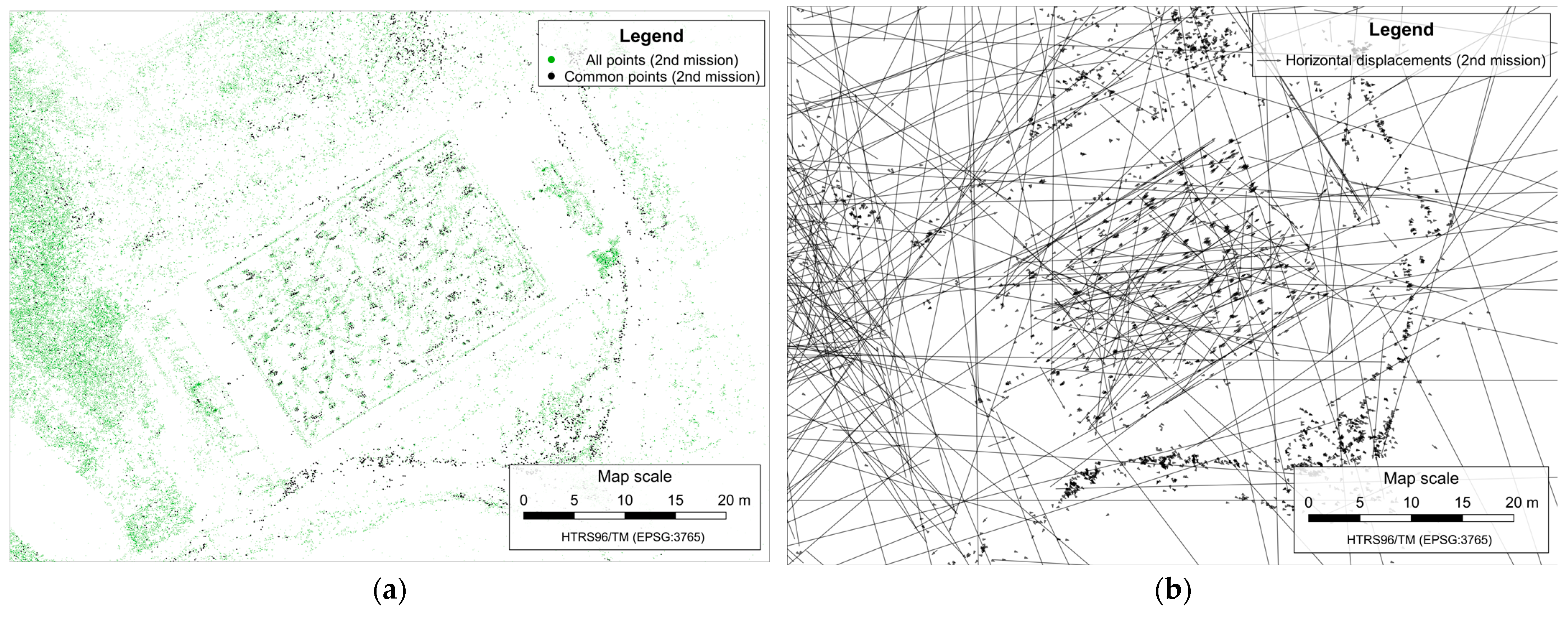
Figure 6a), and in the second mission decreased from 72,531 to 19,125 (26.4%) (
Figure 7a).
The displacement determination is based on comparing the reconstructed sparse point clouds of the same mission from the two surveying epochs by calculating the differences between the coordinates of common matching feature points according to Equation (1). The horizontal displacement vectors determined between all common matching feature points in both missions are shown in
Figure 6b and
Figure 7b.
Before running the outlier removal process, the dataset is filtered keeping only the vectors between feature points found on at least five images in both epochs within each mission and located within the area of simulated landslide, resulting with reduction of the number of displacements vector from 16,339 to 722 (
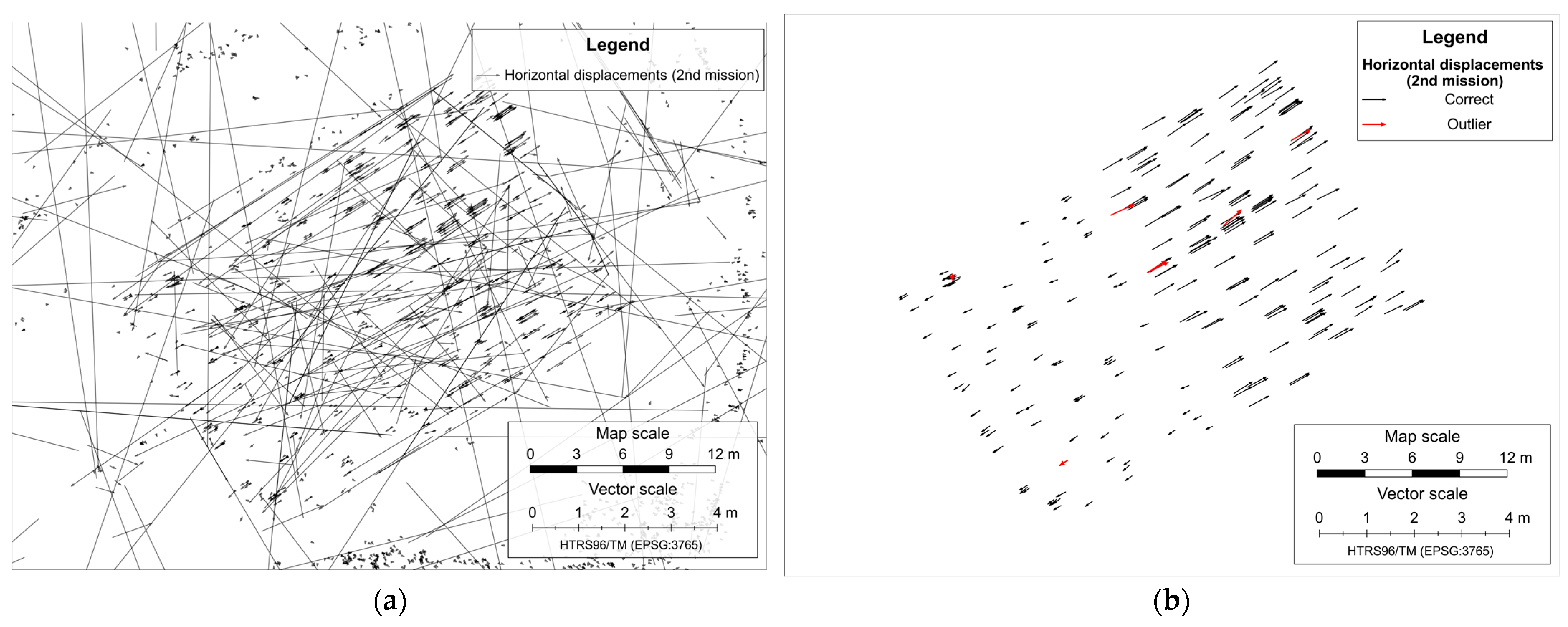
Figure 8a) in the first mission and from 19,125 to 304 (
Figure 9a) in the second mission.
Before removing outlier displacement, additional filtering was performed to discard all displacement vectors whose 3D displacement magnitude is greater than a predefined threshold. In the case of the test field, this threshold was subjectively defined as 1 m, which was approximately twice the maximum magnitude of the simulated displacement between epochs. After performing this filtering, the total number of displacement vectors decreased from 722 to 526 in the first mission, and from 304 to 284 in the second mission.
When the dataset was filtered, removing the remaining outlier displacement vectors from datasets was conducted by performing the iterative LOOCV outlier-removing process based on the kriging interpolation method, as explained in
Section 2.2.
After removing outliers, the total number of displacement vectors remaining was 482 in the first mission (
Figure 8b) and 277 in the second mission (
Figure 9b). The density of the remaining displacement vectors per square meter of simulated landslide area was 0.8 vector per m
2 in the first mission and 0.46 vector per m
2 in the second mission.
As it can be noticed from above-presented results, the number of displacement vectors in the dataset significantly decreased after performing the filtering of data, and detecting and removing outlier from data, but at the same time, the most reliable displacement vectors within the area of the simulated landslide were kept.
3.2. Test Field—The Accuracy of Displacement Determination Using the Proposed Data Processing Method
The remaining displacement vectors were used to generate a displacement map of simulated landslides for each mission, which was made by performing a kriging interpolation based on the datasets that consists of a displacement determined by the proposed data processing method. The interpolation was made on regular raster grid points with a cell size of 1 m, covering the area of the simulated landslide. The displacement maps of the simulated landslide are shown in
Figure 10a and
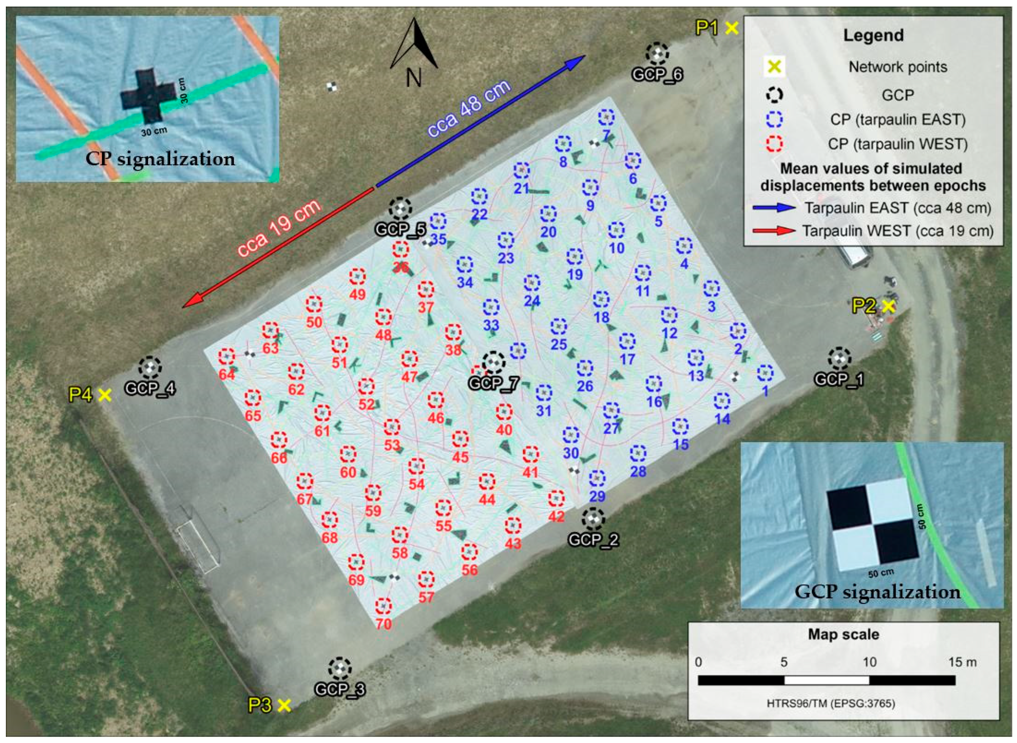
Figure 11a, where it can be seen that the displacements determined by using the proposed data processing method follow the reference displacements (obtained from the measurements with the total station) in magnitude and direction. Accuracy analysis of landslide displacement determination by using the proposed data processing method is performed by comparison of the displacement for all 70 CPs calculated from the total station measurements (which present referent displacement values) and determined displacement vectors of the proposed data processing method based on kriging interpolation with the origins in the same positions.
The range values of displacements in each mission in the east and north directions differ from zero (
Table 5), indicating that the tarpaulins did not move uniformly along the entire surface. However, this is normal because it is impossible to move the entire tarpaulin manually on a flat surface and expect that the displacements over its entire surface at each point will be equal to each other. The reference displacement values in
Table 5 indicate that the average horizontal displacement of the east tarpaulin was 48.2 cm in the north-east direction (59.0°). For the west tarpaulin, it was 18.9 cm in the south-west direction (242.4°). The average vertical displacement value for both tarpaulins indicates that they did not move in height (equal to zero). The determined displacement values are similar to the reference values in both missions. Thus, it can be seen that the mean determined vector values in both missions did not differ by more than 1.2 cm in magnitude and by more than 0.8° in the horizontal angle direction, and also did not differ by more than 0.2 cm in the vertical direction, compared to the reference values.
Displacement residuals are the difference between the reference value and the value of displacements determined using the proposed method (
Table 6). The residuals range from −4.3 cm to 3.7 cm in the horizontal direction and from −2.8 cm to 1.8 cm in the vertical direction.
Table 6 shows that the first mission, in which the UAS operated at a lower flight altitude and achieved more precise results, with mean values of residuals of 0.2 cm in the East direction, −0.1 cm in the North direction, and 0.2 cm in the vertical direction, compared to the results from the second mission, which had mean values of 0.6 cm in the East direction, 0.5 cm in the North direction, and 0.1 cm in the vertical direction.
Figure 10b and
Figure 11b provide the mission-specific graphical representations of the displacement residuals. The graphical representation of the displacement residuals for each mission can be seen in
Figure 10b and
Figure 11b, respectively.
The Root Mean Square Error (RMSE) is used as an indicator of the accuracy of displacement determination using the proposed data processing method. It represents the square root of the sum of the squares of the differences (residuals) between the determined (proposed data processing method) and reference (total station) coordinates of the identical CPs, and it is calculated for each coordinate direction by means of the following equations:
where:
—reference value,
—determined value,
i—index of the CP .
The summary of the achieved RMSE values of displacement determination by using the proposed data processing method for each coordinate direction, horizontal (2D) direction, and spatial (3D) direction for both UAS missions can be seen in
Table 6.
The results in
Table 6 indicate great accuracy of displacement determination with the proposed data processing method because in both missions, the RMSE value for all coordinate directions (1D) was maximally 1.4 cm. The accuracy of the determination of 2D displacements equals 1.0 cm in the first mission and 1.8 cm in the second mission. Furthermore, the accuracy of determination of 3D displacements equals 1.2 cm in the first mission, and 1.9 cm in the second mission, which indicates a good accuracy.
3.3. Test Field—Displacements Determined from Orthomosaics Images
After the displacements were determined using the proposed data processing method, the same displacements simulated on the test field were determined by using a commonly used method based on comparing manually tracked features of SfM-MVS derived orthomosaics from different epochs. This was performed to analyze the possibility to determine displacement vectors with the same accuracy using the proposed data processing method.
Orthomosaic images are produced using OpenDronMap (ODM) v2.9.0 software [
49] based on the sparse point clouds that are generated during the determination of the displacements using the proposed method. Since the surveys in two UAS missions were made twice in different time epochs (before and after simulating displacements), it resulted in the production of four orthomosaics (
Figure 12).
The achieved GSD values of generated orthomosaics was 1.4 cm/px in the first mission and 3.3 cm/px in the second mission. The determination of simulated landslide displacements was performed based on comparing the manually tracked features on SfM-MVS-derived georeferenced orthomosaics resulting from different UAS survey epochs. When tracking the features manually, it is necessary that the chosen features on orthophotos be distinctly recognizable between the epochs. For this purpose, we used clearly recognizable cross marks on the tarpaulins where the center of the cross also marks the position of the CP (
Figure 3). Each tracked feature on the orthomosaics denotes the center of the cross, and horizontal displacement vectors were calculated based on determining the coordinates and their differences between the epochs.
The accuracy of the method based on the comparison of orthomosaic images was performed by calculating displacement residuals as a difference between referent and displacement values determined from orthomosaic images (
Table 7). Since both values denote the displacements between the center of the same cross marks (CPs) on the tarpaulins from different epochs, a comparison was conducted directly i.e., it was not necessary to perform kriging interpolation, as it was performed for calculating displacement residuals for displacements determined by using the proposed data processing method.
The residuals in the horizontal direction range between −5.4 cm to 7.5 cm, and from the results shown in
Table 7, it can be seen that more precise results were achieved in the first mission with lower (50 m) flight altitude.
The results of the accuracy in determining the displacements from orthomosaic images indicate good accuracy, because in both missions, the RMSE value for each coordinate direction was lower than 2.3 cm. The RMSE of determining the horizontal displacements equals 2.2 cm in the first mission and 2.9 cm in the second mission. When compared to the achieved accuracy of the proposed data processing method (
Table 6), it can be noticed that the simulated landslide displacements were determined more accurately by using the proposed data processing method. Moreover, it should be noted that the vertical displacement vectors can be determined using the proposed data processing method, which is not possible from orthomosaic images.
3.4. Case Study—The Accuracy of Displacement Determination Using the Proposed Data Processing Method on the Kostanjek Landslide
Processing of the captured images during two UAS photogrammetric surveys of the Kostanjek landslide using the proposed data processing method was carried out according to the steps described in
Section 2.1. The first step in data processing was to detect features on images collected in both UAS survey epochs. The total number of 196,428,504 features were found on all 2092 images from both surveys, which gives an average of 93.85 thousand features detected per image. From the total number of found features, 23.81% of found features are related to the first epoch, and the other 76.19% are related to the second epoch. The ratio is 1 to 3.2, which is expected because almost three times more images were captured in the second epoch.
The next step of the proposed data processing method is feature matching. A total of 29.02 million matches are found among all images where over 2.19 million are common matches between epochs. The next step was the matching of the feature points. The total number of matching feature points equals to 7,529,936, while 675,485 of them are detected on images from both epochs.
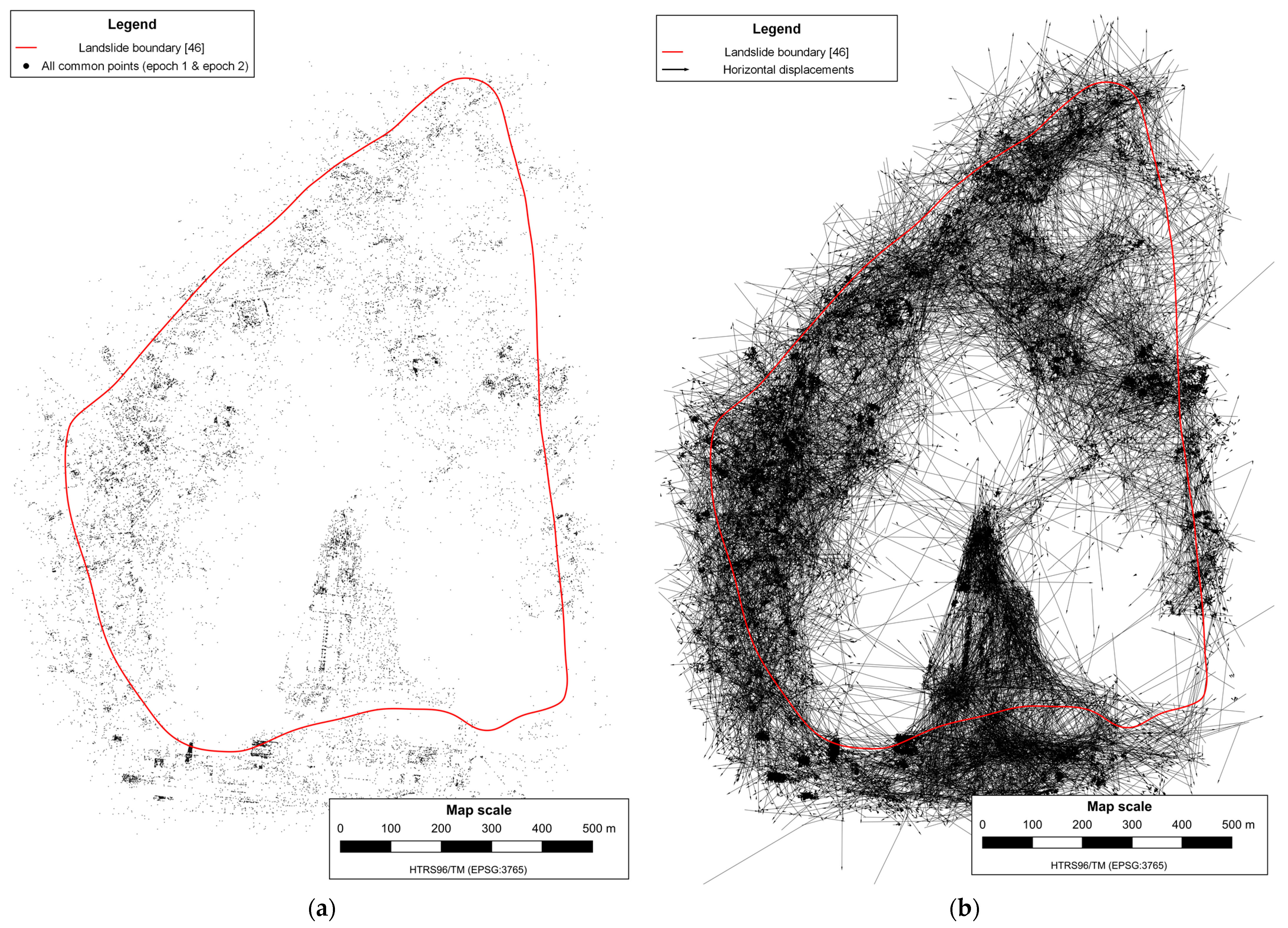
After the feature matching process, SFM reconstructions were executed independently for each epoch. One reconstruction was based solely on the features and matches between images from the first epoch, and the other was exclusively based on features and matches between images from the second epoch. After the SfM reconstructions, the number of common matching feature points decreased from 675,485 to 33,545 (5.0%) (
Figure 13a). The next step was calculating the displacements based on the comparison of reconstructed sparse point clouds from two survey epochs by calculating the differences between the coordinates of common matching feature points (
Figure 13b) using Equation (1).
As explained in
Section 2.1, the dataset is filtered before running the outlier removal process, keeping only the vectors between feature points found on at least five images in both epochs, resulting in the reduction of the number of displacements vector from 33,545 to 5657 (
Figure 14a). After removing outlier displacement vectors (
Figure 14b) from datasets by performing LOOCV processes based on the kriging interpolation method, the total number of displacement vectors that remained was 1822.
The displacement map of the Kostanjek landslide was prepared by performing kriging interpolation, where the interpolation was based on the displacement dataset that consists of a displacement determined by using the proposed data processing method. The points on which the displacement vectors were determined are the points of a regular raster grid covering the landslide area. The landslide map can be seen in
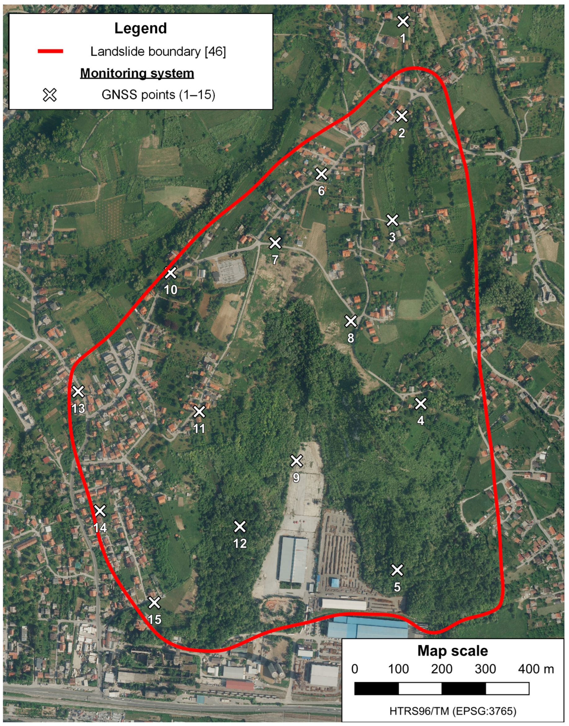
Figure 15a, indicating that the determined displacements successfully follow the actual displacements in magnitude and direction (red vectors show actual displacements determined with the measurements of 15 GNSS monitoring system sensors).
The proposed data processing method is validated by comparing its determined displacement vectors with the displacement vectors determined in the measurements with the GNSS monitoring system sensors and their values are considered as reference values. In order to consider the comparison as valid, the vectors being compared must have their origin at an identical position. Since the origins of the reference displacement vectors refer to the positions of the GNSS sensor in the first epoch, it is necessary to determine the displacement vectors of the proposed data processing method based on kriging interpolation in the same positions. The kriging interpolation was used to predict displacement vectors at the position of the GNSS sensors based on the displacement dataset determined by means of the proposed data processing method. Thus, out of 15 GNSS sensors of the monitoring system of the Kostanjek landslide, 14 were used as CPs in the validation process. One GNSS point (GNSS 01) was placed outside the landslide area, and therefore, it was not used in the validation process. Displacement residuals are calculated as a difference between referent and displacement values determined by using the proposed method (
Table 8).
The statistics results in
Table 8 show that the residuals in the east direction ranged between −5.0 cm and 6.5 cm, with a mean value of −0.2 cm; and in the north direction, they ranged between −4.7 cm and 5.5 cm, with a mean value of 0.1 cm; and in height, they ranged between −4.7 cm and 8.7 cm, with a mean value of 1.2 cm. The graphical presentation of the displacement residuals is shown in
Figure 15b.
According to the results shown in
Table 8, it can be concluded that the displacement vectors are determined with reasonable accuracy since the RMSE values of the determined horizontal (2D) displacements equal 4.0 cm, and the RMSE value of the determined spatial (3D) displacements equals 5.4 cm. These accuracies represent an acceptable result since the flight altitude was higher by 40 m in the first epoch than in the second epoch, and the camera used for the acquisition of images in the first epoch had a shorter focal length than the camera in the second epoch, leading to a significant difference in image GSD values between the epochs (GSD(epoch 1) = 4.1 cm/px, and GSD(epoch 2) = 2.6 cm/px).


