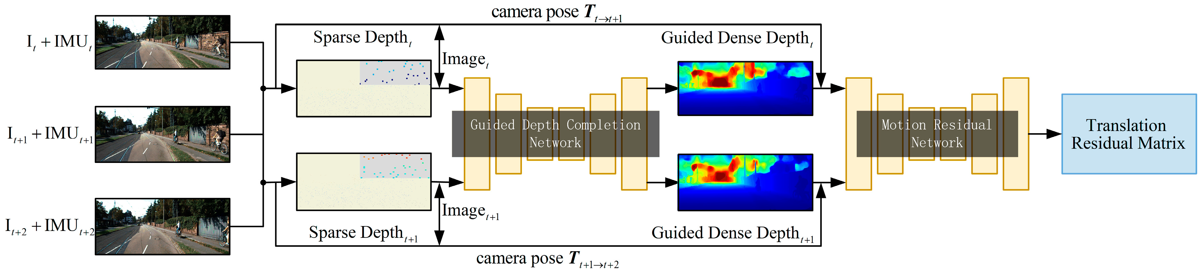
Specifically, we used VI-SLAM (see
Section 3.1) to calculate the depth of feature points in the scene and the motion pose of the cameras. The sparse depth map and RGB images were used as the guidance depth complement network input to make the network output guidance dense depth (see
Section 3.2). In addition, the dense depth, RGB images and camera motion pose were used as the input of the motion residual network to make the network predict the motion of each pixel relative to the background (see
Section 3.2). We proposed a new regularized loss function (see
Section 3.3), which is helpful for training in highly complex dynamic scenes.
3.2. Depth and Motion Networks
The depth and Motion networks are mainly divided into two parts. The first part is the guidance depth completion network used to estimate the dense depth, and the second part is the motion residual network used to estimate the object motion.
Inspired by Eldesokey et al. [
14],
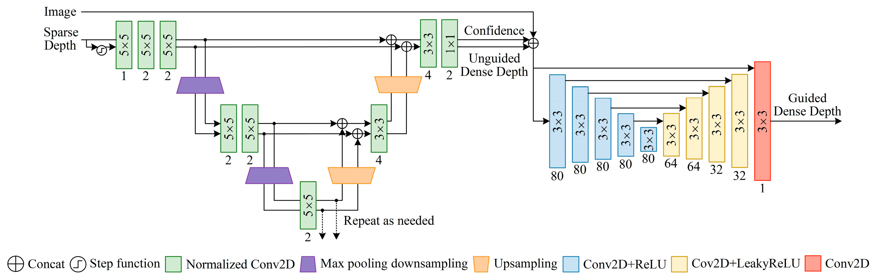
Figure 2 shows a new network of depth completion. This is a layered multi-scale architecture. The architecture acts as a generic estimator for different scales and gives a good approximation for the dense output at a very low computation cost. In the first stage, we used the normalized convolution model. The concept of normalized convolution was proposed by Knutsson and Westin based on the signal theory with confidence [
26]. The core advantage of normalized convolution is the separation between signal (depth) and confidence. We only needed to provide an initial confidence. Through continuous normalization convolution, we can adaptively process this confidence and determine the final confidence of the output and the unguided dense depth. At the same time, the output confidence can also reflect the density of input confidence. We refer to the method of outputting confidence in the literature [
27]. In our network, in order to obtain the initial confidence, we calculated the step function of the sparse depth image. That is, the confidence level for pixels with depth value was set to 1, and the confidence level for pixels without depth value was set to 0. In addition, in order to fuse different scales, the output and corresponding confidence of the last normalized convolution layer were unsampled using the nearest neighbor interpolation, and connected with the corresponding scale through jump connection. Because of the dense depth learned from the sparse depth images estimated by VI-SLAM, it shows weakness in the local area of weak textures. Therefore, this problem was mitigated in the second stage by using RGB images and new forms of auxiliary data fusion. The auxiliary data were the confidence level of the first stage output that holds the reliability of the depth value of each pixel. We will prove in subsequent experiments that the accuracy of depth complement is improved by assisting RGB image fusion with output confidence.
The input of the motion residual network is a pair of consecutive frames connected along the channel dimension. The motion residual network is similar to the network in reference [
28]. The difference is that each input image has five channels: RGB channel, guided dense depth channel and motion pose channel. The output of the motion residual network is the translation residual matrix
, which represents the translation size of the dynamic objects in the pixel coordinate system.
According to the dense depth
of the current frame outputted by the guidance depth complement network, and the motion pose of two adjacent frames provided by visual-inertial system, the pixel coordinate
of each pixel point of the current frame in the next frame image are:
where
is the internal parameter of the cameras, and
is the depth value of each pixel of the predicted next frame image.
Equation (1) only considers the pixel change caused by camera motion, and does not consider the pixel change between two frames caused by the motion of the dynamic object itself in the scene. As shown in Equation (2), the accurate pixel coordinate
and the corresponding pixel value
of the next frame image of the dynamic object can be obtained through the translation residual matrix output by the motion residual network.
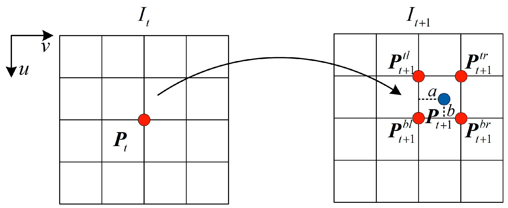
Meanwhile, as shown in
Figure 3, in the process of projection reconstruction between two frames, the pixel value
of each pixel point of the reconstructed images can be obtained through the differentiable bilinear interpolation method [
25]:
3.3. Losses
Since our goal was to only use VIO for depth completion and dynamic object motion learning in dynamic scenes, a lot of regularization of loss functions was required during training. In particular, we explicitly considered the problem of occlusion in order to eliminate the occlusion interference in the unsupervised training of depth completion, and designed the corresponding loss functions for different situations in the occlusion area. Starting from analyzing different situations of occluded areas, we describe the following loss functions, which are the key contributions of this work.
Through the RGB images and the translation residual output of motion residual network, the pixel coordinate
and the corresponding pixel value
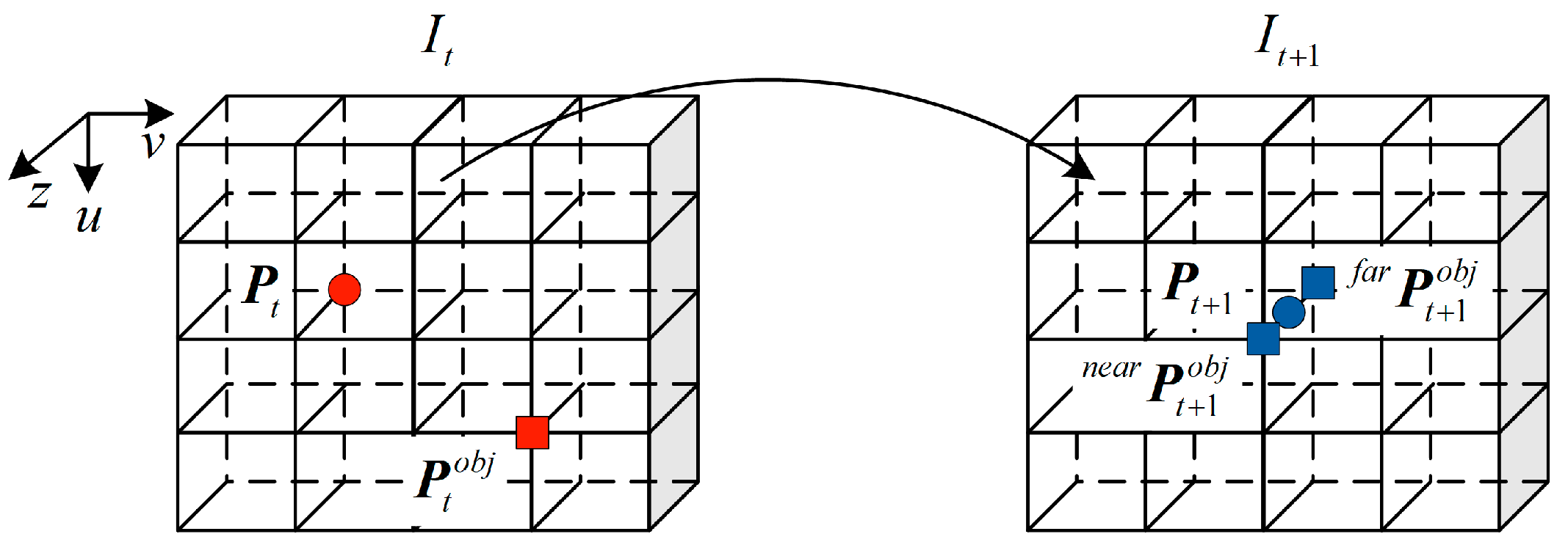
of the dynamic object at the current time can be obtained. The dynamic object area at the current time is defined as a dynamic area, and the static structure area at the current time is defined as a static area. When the current frame images are projected to the next frame, due to the motion of the cameras and the dynamic objects, there will be an area occluded by each other. This area is defined as an occluded area. As shown in
Figure 4, occlusion conditions in the occlusion area are mainly divided into two types: the depth of static structures are smaller than dynamic objects and the depth of static structures are larger than dynamic objects.
According to Equation (2), the pixel coordinate
of the next frame image of the dynamic objects and the pixel value
of the corresponding RGB images can be obtained. Note that the key point at this time is to determine whether the pixel belongs to the dynamic object or the static scene. According to Equation (4), the pixel coordinate
can be projected back to the pixel coordinate
of the current frame, and the corresponding pixel value
can be obtained from the RGB images.
Next, we identified the category of occlusion by judging the pixel difference between or . If the former is smaller than the latter, then the static structure depth is small. That is, static structures are not occluded and dynamic objects are occluded. At this point, pixels in the occluded area are naturalized to pixels in the static area. On the contrary, the static structure depth is larger, and the pixels of the occluded area are naturalized to pixels of the dynamic area. Similarly, when multiple dynamic objects move to the same pixel, the pixel difference of these dynamic objects and static structures can be used to identify which of them pixel value of the pixel belongs to.
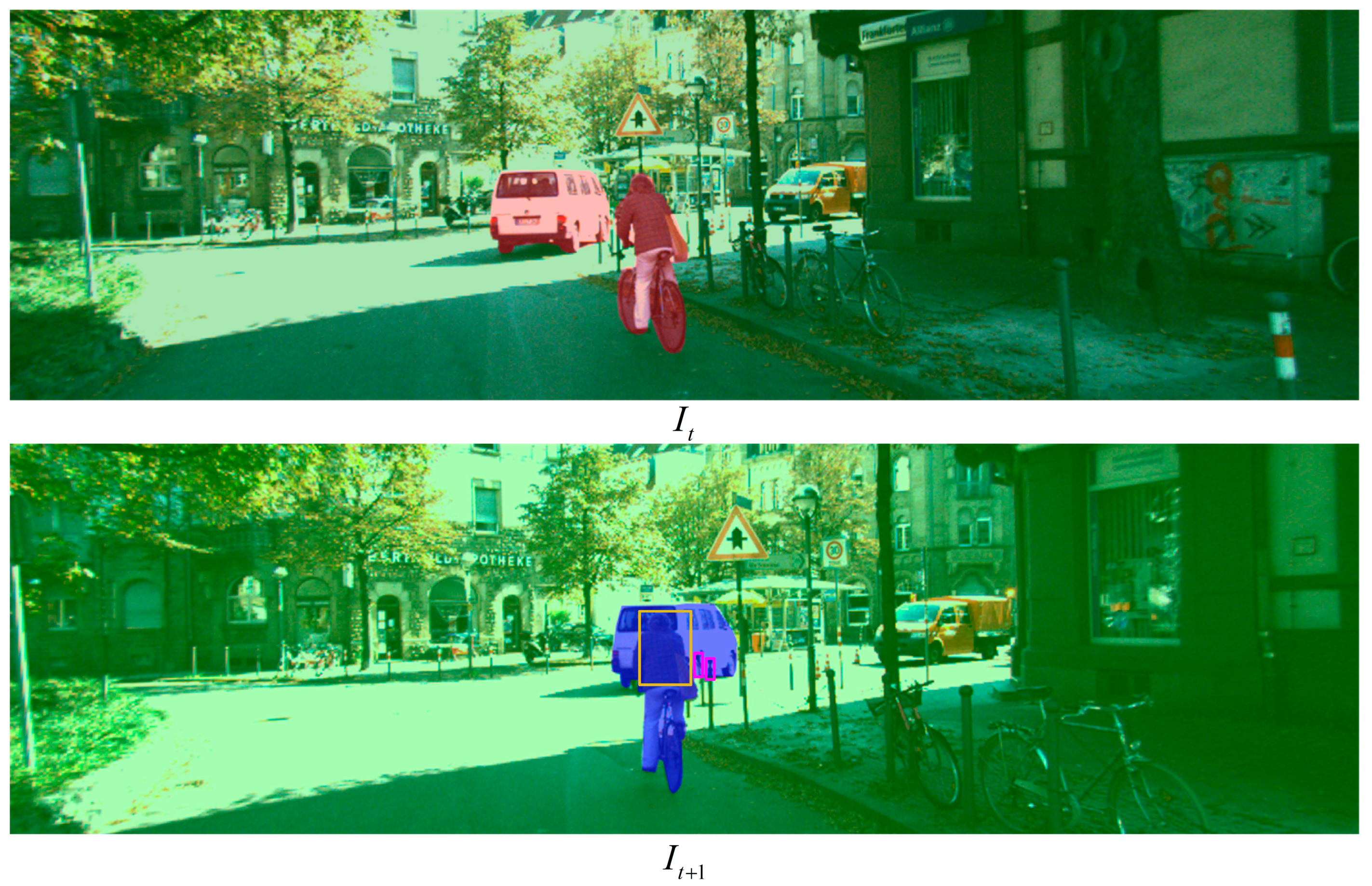
As shown in
Figure 5, we listed a group of schematic diagrams of pixel region classifications of two adjacent frames. Through the motion residual network, the dynamic area at the current time can be obtained (marked by red shadow), and the static area at the current time can be marked by green shadow. At the next moment, we can judge the occluded area (marked by blue shadow) through the above description, in which the pink box is static structure occluding dynamic structure, the orange box is dynamic structure occluding each other, and the rest is dynamic structure occluding static structure. In training, the pixels in the pink box belong to the static area, and the rest belong to the pixels in the dynamic area.
The translation residual
of the residual translation network output is regularized normalized by the
loss function. In order to keep the motion of all pixels belonging to a dynamic object consistent, the translation difference of each dynamic object in the dynamic region using the
loss function is minimized. It is defined as:
The dense depth
of the depth complement network output is normalized by the photometric consistency losses and parallax smoothing losses that are complementary to the maximum confidence. The luminosity loss consistency is a combination of
penalty and SSIM [
29] for average reprojection error of each pixel, and SSIM is a perceptual measure of the constant change of local illumination. Parallax smoothing losses are the standard edge perception smoothing regularization of parallax map
. It ensures that the loss weight of parallax smoothing is small when the images gradient is large. Specifically, the photometric consistency losses are calculated as shown in Equation (6) for pixels in the static region. The photometric consistency losses are calculated as shown in Equation (7) for pixels in the dynamic region. The parallax smoothing losses are calculated as shown in Equation (8) for all pixel points.
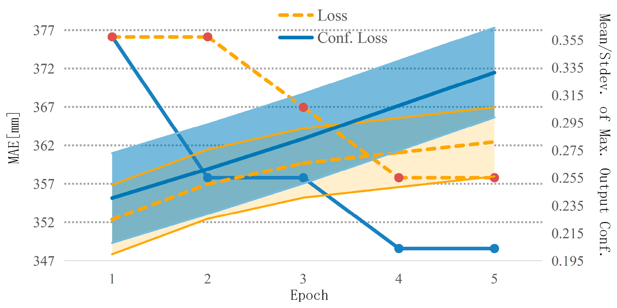
In the supervised depth completion network with normalized convolution layer, it is necessary to maximize the output confidence
while minimizing the data error. Therefore, it is necessary to realize the loss functions of these two objectives at the same time. The total losses
:
where
is the epoch number. The confidence term is decaying by dividing it by the epoch number
to prevent it from dominating the losses when the data error term starts to converge.


