4.1. Lidar Wind Power Data Collection
At present, most wind farms use the method of building an anemometer tower to observe the wind conditions at the site continuously around the clock, and then record and store the measurement data in the data recorder installed on the tower body. However, the anemometer tower has disadvantages, such as many requirements for site selection, difficult maintenance, and high cost, which bring huge investment risks and loss of income to the construction, operation, and maintenance of wind farms. Lidar has the advantages of light and portable, easy installation, simple operation, and accurate wind measurement results. It is currently widely used in the field of wind power at home and abroad.
Wind Iris is the first wind turbine nacelle wind lidar developed by the French company Leosphere (Paris, France). It can measure the wind speed and wind direction in the range of 40~400 m directly in front of the hub of the wind turbine. Real-time data and statistics can be automatically transmitted via the data protocol or stored on the device itself. Wind Iris emits two laser beams at the same time to measure the wind speed at the hub height in front of the unit, and the wind speed measured by the two laser beams is processed to obtain the actual wind speed at the hub height at the measured position. However, Wind Iris cannot measure data such as wind direction, air pressure, temperature, and humidity.
The WindCube V2 land-based lidar is also developed by Leosphere (Paris, France). The wind speed, wind direction, and other indicators are measured by measuring the frequency change in the moving speed of the aerosol in the air by the pulsed laser. Measuring equipment such as air pressure, temperature, and humidity are embedded in the lidar wind measurement system. The WindCube V2 lidar emits four laser beams at the same time, measures the wind speed at four points within each layer height, performs weighted processing, and obtains the average wind speed and wind direction of the layer height.
Both lidars use laser pulse Doppler. The principle of frequency shift, by measuring the Doppler frequency shift generated by the aerosol backscatter echo signal; accurate real-time wind field data; and aerosol backscatter data are obtained to invert wind speed and wind direction information [
37,
38]. The specific working principle is as follows:
Let the laser-emitting module and the receiving module be used as the inertial system S, and the measured object be used as the inertial system A; the motion speed of the inertial system A relative to the inertial system S is
. When the laser source emits a beam of laser light with frequency
to the measured object, in the inertial system A, the laser frequency at the measured object is:
The emitted laser light is backscattered by aerosol particles, and part of the light is reflected back to the detector. In the inertial system S, the laser frequency at the receiving module is:
Therefore, there is a frequency difference between the local oscillator light and the echo signal, and the frequency difference is the Doppler frequency shift, namely:
The above Doppler frequency shift formula is applicable to the off-axis coherent wind lidar system. For the transceiver coaxial system, the laser transmitting module and the receiving module are the same telescope,
, Formula (23) can be simplified as:
Among them, is the laser wavelength, is the moving speed of the measured object, and is the angle between the measured object and the emitting laser.
4.4. Experimental Results and Model Comparison
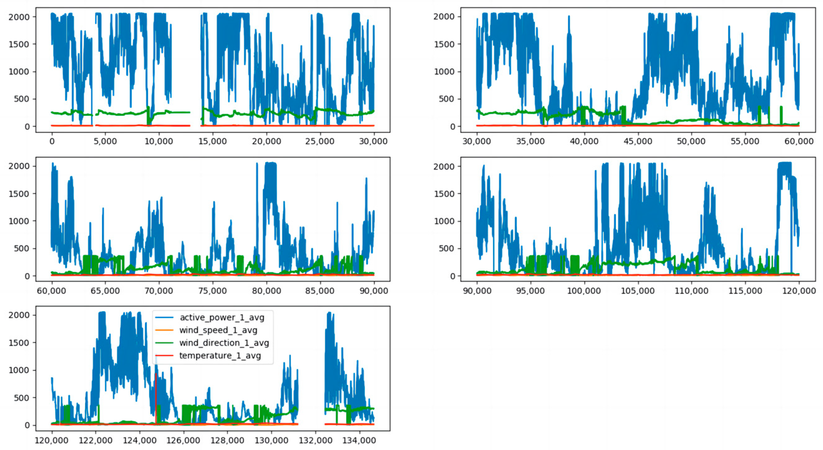
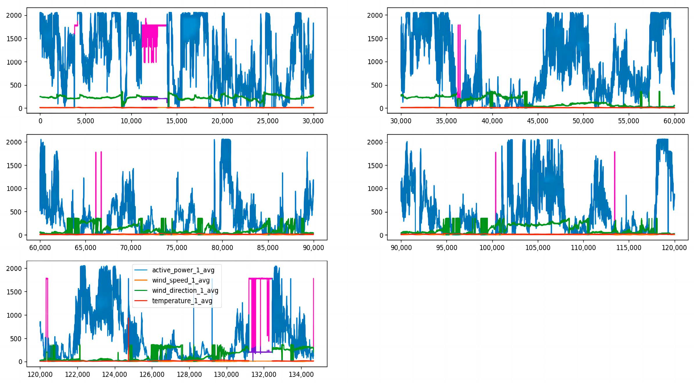
Since the CGAN-CNN-LSTM model is relatively advanced, it is meaningless to compare it with the BP neural network, Elman neural network, and other prediction models, so the CNN-LSTM, LSTM, and SVM prediction models were selected for comparative experiments. First, we imported all the data sets. From
Figure 6, it can be seen that the data in the first part and the data in the fifth part are obviously missing.
Figure 7 shows the effect after supplementing the data with the CGAN correlation, data supplements have been highlighted in different colors.
We selected February, May, August, and November from the one-year data set, 5 days per month as the training set, and 1 day as the test set. Fans 1, 3, 5, and 7 were selected as test units. The wind speed, wind direction, and temperature in the NWP data are used as the input data, and the output is the wind power.
Figure 8 shows the influence of the wind speed, wind direction, and temperature on the wind power, among which wind speed has the greatest influence, and wind direction has the least influence.
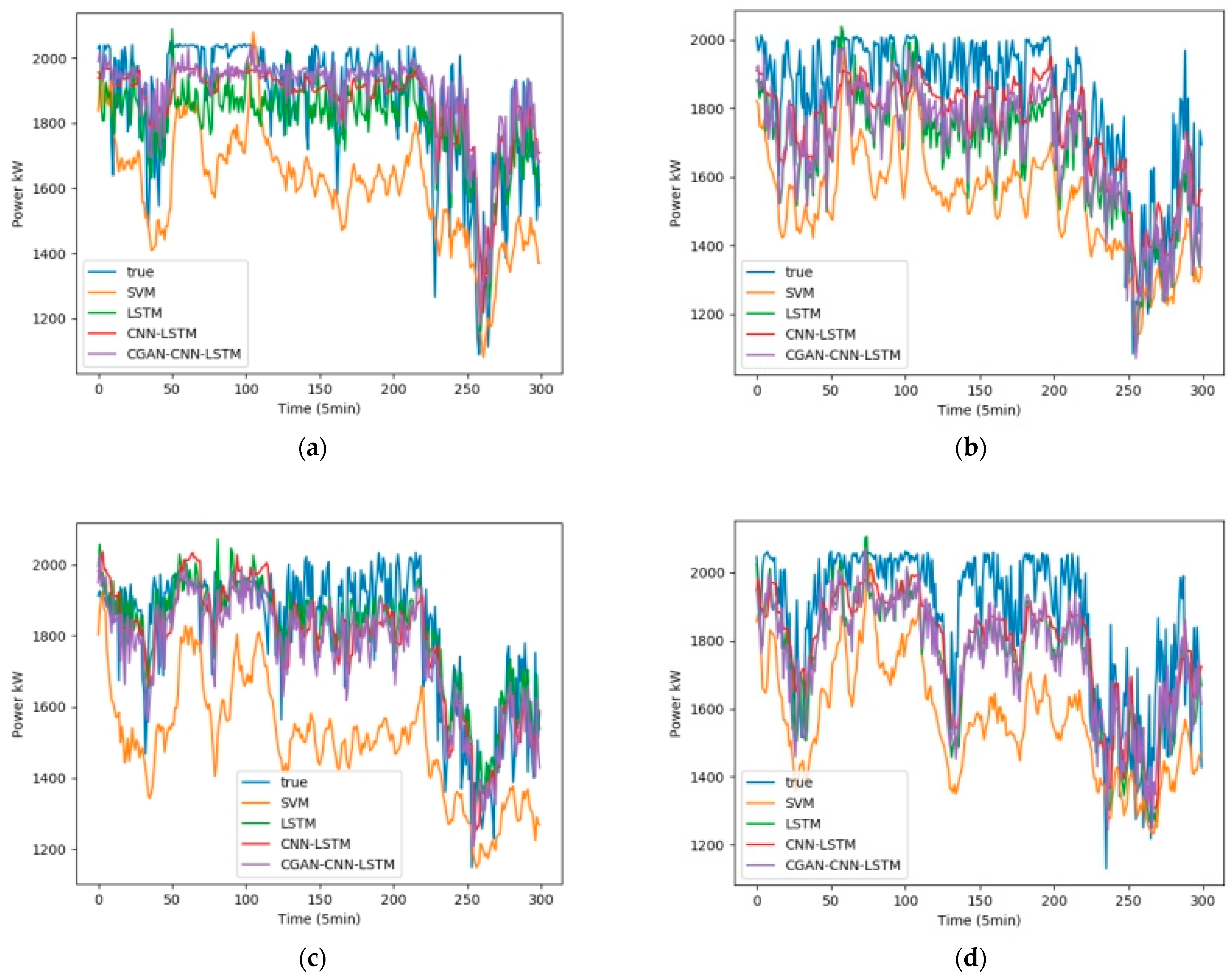
Figure 9 shows the test results in February,
Figure 10 shows the test results in May,
Figure 11 shows the test results in August, and
Figure 12 shows the test results in November. In the simulation diagram, the 300 sampling points in the image are divided according to the time scale, and a sampling point every 5 min predicts the wind power of a day.
Table 2 shows the data of the two loss functions of
and
of the four forecasting models in February, and
Table 3,
Table 4 and
Table 5 represent the same content in May, August, and September, respectively.
It can be seen from
Table 2 that the average values of
of the four prediction models of CGAN-CNN-LSTM, CNN-LSTM, LSTM, and SVM are 0.934, 0.922, 0.911, and 0.847; the average values of
are 0.0804, 0.0871, 0.0939, and 0.1236, respectively.
It can be seen from
Table 3 that the average values of
of the four prediction models of CGAN-CNN-LSTM, CNN-LSTM, LSTM, and SVM are 0.911, 0.873, 0.888, and 0.891; the average values of
are 0.0733, 0.0872, 0.0826, and 0.0783, respectively.
It can be seen from
Table 4 that the average values of
of the four prediction models of CGAN-CNN-LSTM, CNN-LSTM, LSTM, and SVM are 0.925, 0.912, 0.899, and 0.898; the average values of
are 0.0710, 0.0739, 0.0785, and 0.0803, respectively.
It can be seen from
Table 5 that the average values of
of the four prediction models of CGAN-CNN-LSTM, CNN-LSTM, LSTM, and SVM are 0.911, 0.887, 0.881, and 0.892; the average values of
are 0.0847, 0.1056, 0.1060, and 0.1001, respectively.
For the whole year, it can be seen from the figure that the forecasts for February and August are better than those for May and November. This is because February and August are windy months, with strong and relatively stable wind speeds, and less fluctuations in wind power power, which are easier to predict. It can also be seen from the figure that the fitting curves of SMV5 and SMV7 are obviously better than those of SMV1 and SMV3. This is because there are a small number of wind speed and temperature in the data sets of SMV1 and SMV3 units. Or the record of the wind direction is missing, which does not match the power value at the same time, resulting in some impact on the power prediction of the model. The final results show that for different wind turbines tested in different months in the same wind farm, The average values of of the four prediction models of CGAN-CNN-LSTM, CNN-LSTM, LSTM, and SVM are 0.921, 0.899, 0.895, and 0.882; the average values of are 0.0774, 0.0885, 0.0903, and 0.0956, respectively. Compared with the best CNN-LSTM in the control experiment, CGAN-CNN-LSTM increased by 2.45% and decreased by 12.5%. It proves that this model is more accurate in predicting wind power.
In order to show that the model is applicable to wind farms all over the world, and to verify the difference between CGAN and general interpolation methods, this experiment adds a set of control experiments in Chinese wind farms. The content of the experiment is to set the data of the wind farm from March 1st to 5th as the training set. The data on March 6 was set as the test set, and the CGAN-CNN-LSTM model and the CNN-LSTM with linear interpolation model (L-CNN-LSTM) were used to make predictions, and the test results of the four machines were compared,
Figure 13 and
Table 6 are the test results in March.
Table 6 is the
and
evaluation functions of these two groups of models.
In experiments in wind farms in China, the final results show that the average value of the CGAN-CNN-LSTM prediction model is 0.927, and the average value of the L-CNN-LSTM prediction model is 0.887; The average value of the CGAN-CNN-LSTM prediction is 0.0812, and the average value of the L-CNN-LSTM prediction model is 0.0926. It can be seen that compared with the L-CNN-LSTM prediction model, the value of this model increases by 4.5% on average, and the value decreases by 12.3% on average, which is closer to the actual wind power curve.


