
Integrating Cosmic Microwave Background Readings with Celestial Navigation to Enhance Deep Space Navigation

 , , and
Abstract
:1. Introduction
2. The Cosmic Microwave Background as a Navigation Reference
3. Methodology for CMB Velocity Determination
4. Preliminary Feasibility Assessment of CMB Measurements for Navigation Purposes
4.1. Foreground Noise
- Galactic Synchrotron Emission: This nonthermal radiation is produced by high-energy electrons spiraling in the Galaxy’s magnetic field [53]. It dominates at low frequencies (under 10 GHz) and can affect the CMB signal at frequencies below 50 GHz. However, its spectral index causes it to decline sharply with increasing frequency, minimizing interference above 70 GHz [51];
- Spinning Dust Emission: This emission arises from the rotational motion of tiny dust grains in the interstellar medium of galaxies [53]. These spinning dust grains, typically a few nanometers in size, emit radiation mainly below 30 GHz as they interact with ambient radiation and magnetic fields [51]; and
4.2. Systematic Errors
- Gain Fluctuations: These are caused by various instrumental and environmental factors during a scan observation. They result in residual calibration uncertainty, which modulates the polarization field and can distort the CMB signal;
- Angle Errors: These arise from thermal deformation, mechanical vibration of instruments, errors in telescope-attitude determination, and inaccuracies in optical system calibration. Such errors affect the alignment of the observed data with the true sky signals; and
- Pointing Errors: These occur when there is a mismatch between the actual pointing direction and its estimated direction, degrading the spatial position accuracy of the observed data.
4.3. Sensors
- Antenna: Captures the CMB signal;
- Dicke Switch: Rapidly alternates between the antenna signal and a reference source, minimizing gain variations;
- Local Oscillator: Generates a stable frequency used for mixing with the input signal;
- Mixer: Combines the input signal with the local oscillator signal, producing the IF signal;
- IF Amplifier: Amplifies the lower-frequency IF signal, reducing noise compared to direct amplification; and
- Detector: Converts the amplified signal to a measurable output.
- Bandwidth: Increasing the bandwidth improves sensitivity but also increases noise. In the Planck mission, a bandwidth of approximately 20% of the central frequency, around 1 GHz for the three selected frequencies, was targeted [67]. Achieving this is feasible but requires high-quality electronics;
- System Noise Temperature: Higher frequencies lead to higher , making it impractical to use this type of equipment for frequencies above 100 GHz for CMB measurements. An appropriate value is approximately 30 K [66]; and
- Integration Time: Longer observation times improve precision. Therefore, a data accumulator can enhance accuracy by averaging the random noise.
- Absorber: Captures the incoming radiation and converts it into heat;
- Thermometer: Measures the temperature change in the absorber; and
- Heat Sink: Maintains a stable reference temperature.
4.4. Preliminary Requirements
- Utilize multi-frequency sensors to mitigate foreground noise;
- Design sensors to be positioned on the spacecraft in a way that favors measurements aligned with the direction of its velocity;
- Implement scan patterns to mitigate systematic errors; and
- Accumulate data onboard to increase the sensitivity of the sensors.
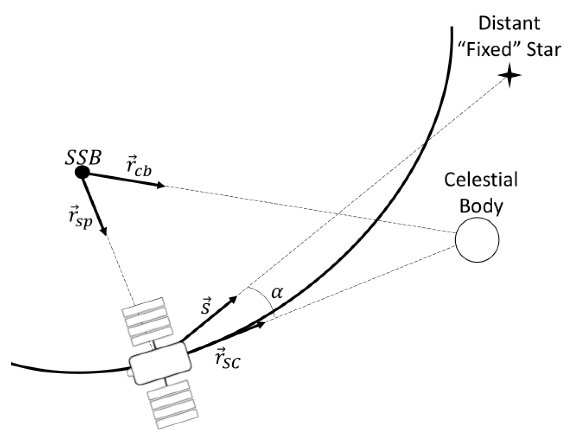
5. Integrating CMB and Celestial Navigation for State Estimation
6. Simulation and Analysis
6.1. Initial Conditions for the Simulation
6.2. CeleNav Method
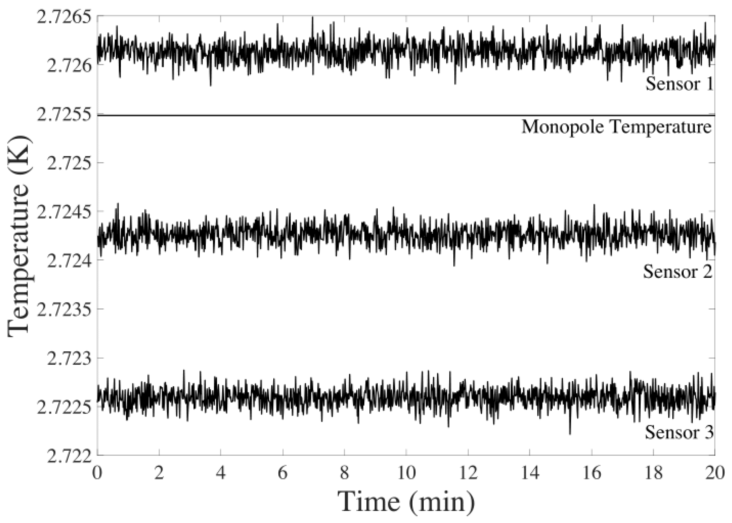
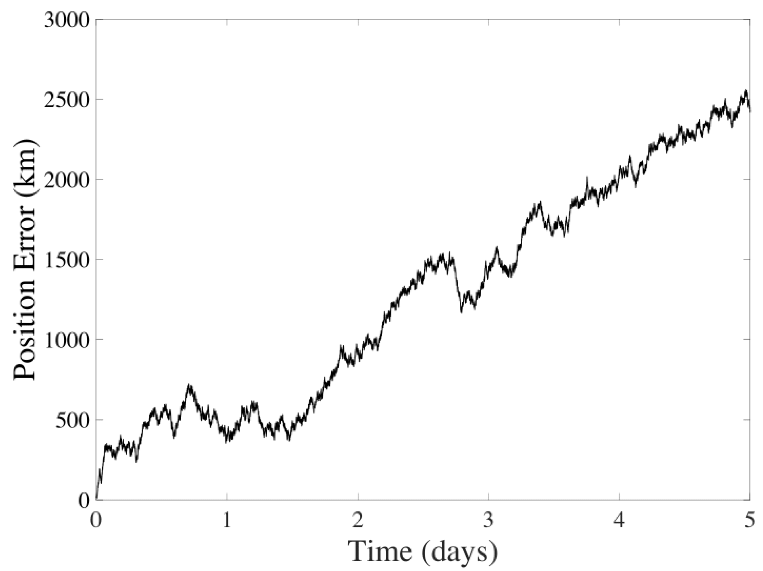
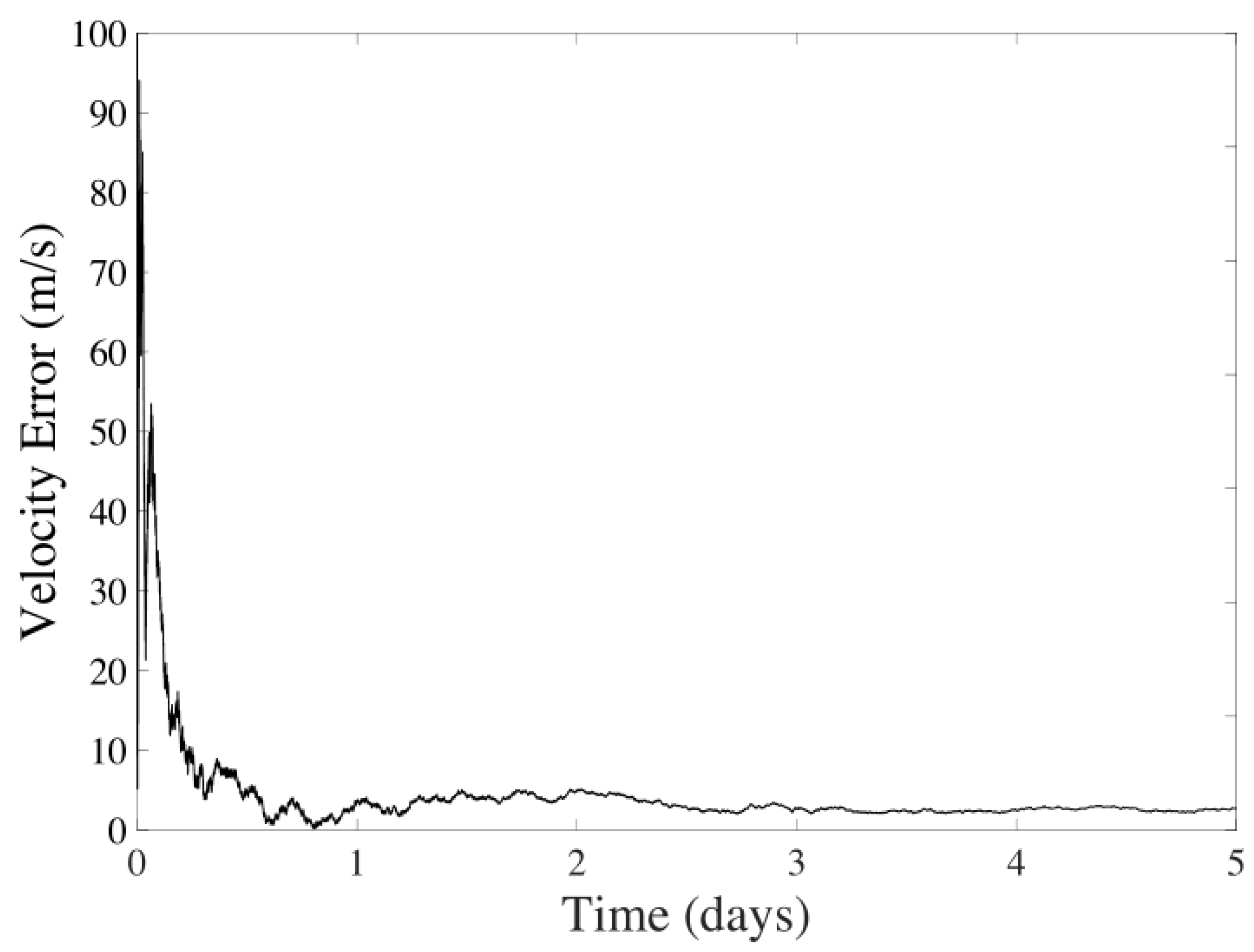
6.3. CMB Method
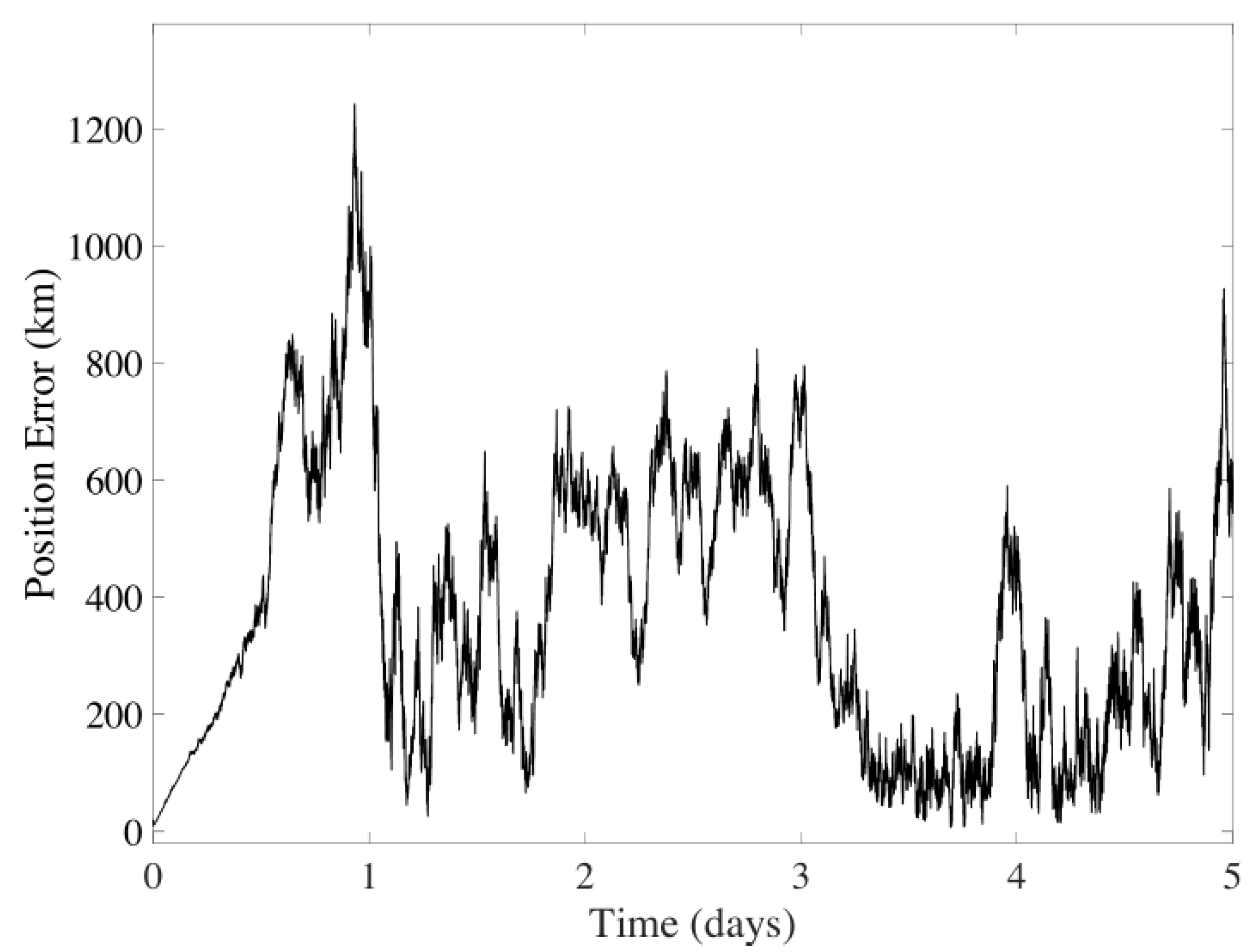
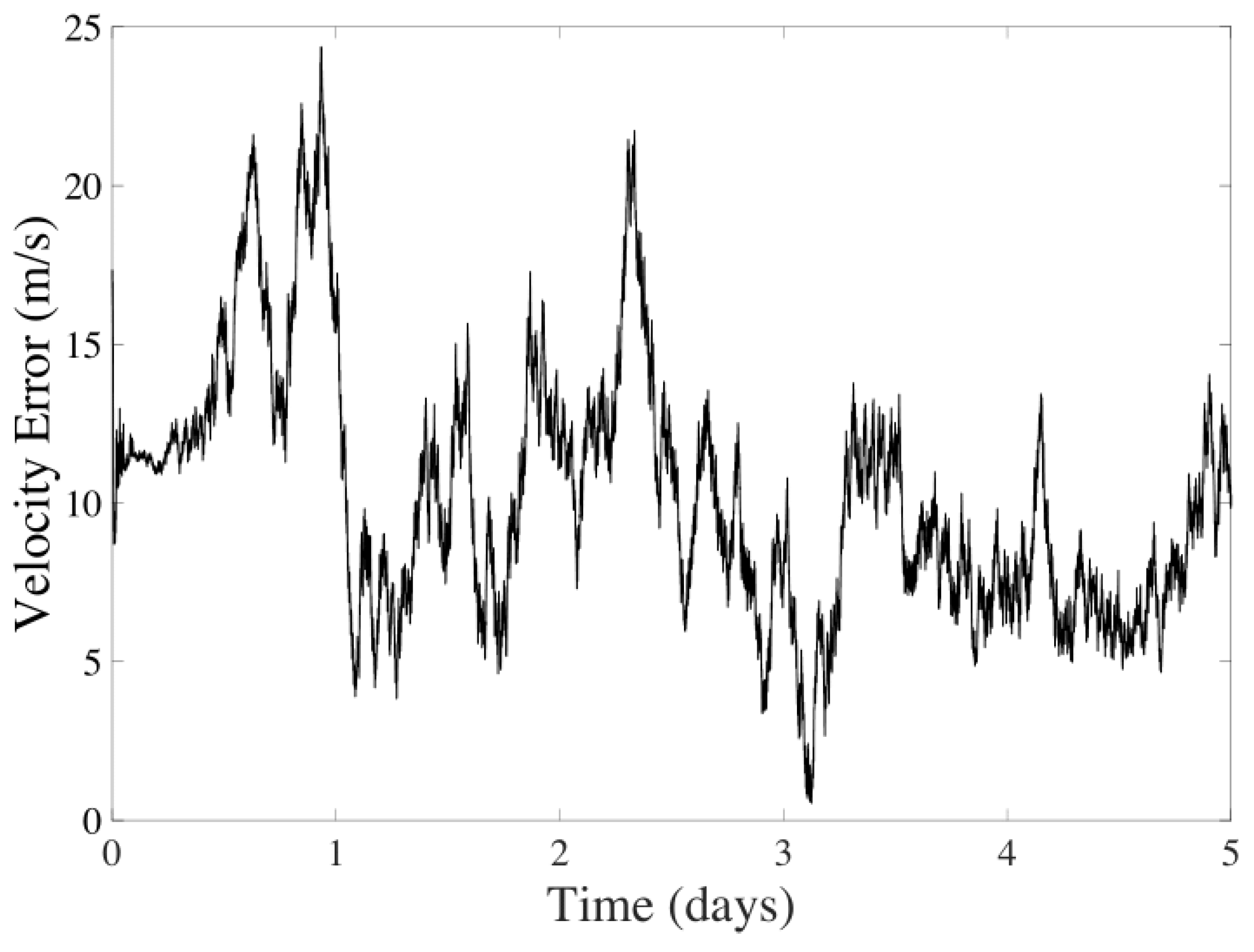
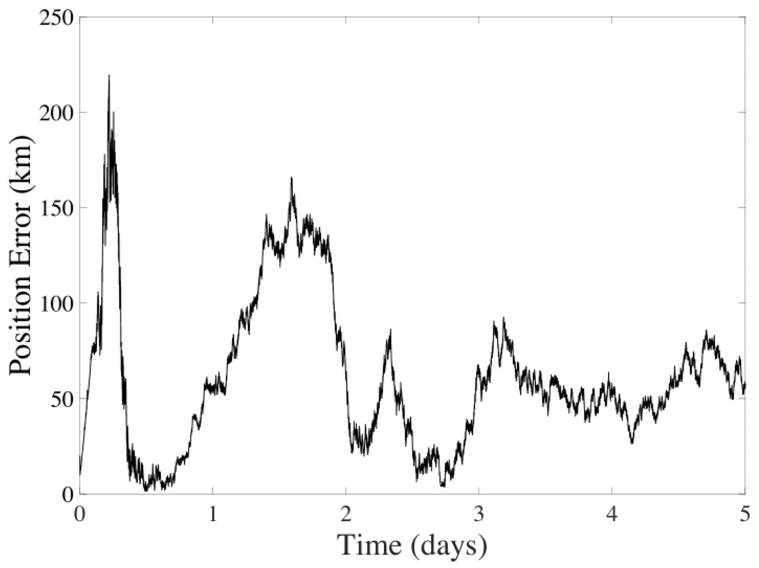
6.4. Hybrid Method
6.5. Analysis of the Three Methods
7. Conclusions
Author Contributions
Funding
Institutional Review Board Statement
Informed Consent Statement
Data Availability Statement
Conflicts of Interest
References
- Deutsch, L.J.; Townes, S.A.; Liebrecht, P.E.; Vrotsos, P.A.; Cornwell, D.M. Deep space network: The next 50 years. In Proceedings of the 14th International Conference on Space Operations, Daejeon, Republic of Korea, 16–20 May 2016. [Google Scholar] [CrossRef]
- Means, H.H. The Deep Space Network: Overburdened and underfunded. Phys. Today 2023, 76, 22–23. [Google Scholar] [CrossRef]
- Turan, E.; Speretta, S.; Gill, E. Autonomous navigation for deep space small satellites: Scientific and technological advances. Acta Astronaut. 2022, 193, 56–74. [Google Scholar] [CrossRef]
- Corrado, L.; Cropper, M.; Rao, A. Space exploration and economic growth: New issues and horizons. Proc. Natl. Acad. Sci. USA 2023, 120, e2221341120. [Google Scholar] [CrossRef] [PubMed]
- Crawford, I.A. Lunar resources. Prog. Phys. Geogr. Earth Environ. 2015, 39, 137–167. [Google Scholar] [CrossRef]
- Jakhu, R.S.; Pelton, J.N.; Nyampong, Y.O.M. The importance of natural resources from space and key challenges. In Space Mining and Its Regulation; Springer: Berlin/Heidelberg, Germany, 2017. [Google Scholar] [CrossRef]
- Zurbuchen, T. Science 2020–2024: A Vision for Scientific Excellence; Technical Report; National Aeronautics and Space Administration: Washington, DC, USA, 2020.
- Deutsch, L.J.; Dowen, A.; Townes, S.; Guinn, J.; Wyatt, E.J.; Levesque, M.; Chang, S. Autonomy for Deep Space Communications and Navigation. In Proceedings of the SpaceOps 2021, Cape Town, South Africa, 3–5 May 2021. [Google Scholar]
- Bhaskaran, S. Autonomous navigation for deep space missions. In Proceedings of the SpaceOps 2012, Stockholm, Sweden, 11–15 June 2012. [Google Scholar] [CrossRef]
- Owen, W.M.J. Methods of Optical Navigation. In Proceedings of the AAS/AIAA Space Flight Mechanics Meeting, New Orleans, LA, USA, 13–17 February 2021. AAS 11–215. [Google Scholar]
- Graven, P.; Collins, J.; Sheikh, S.; Hanson, J.; Ray, P.; Wood, K. XNAV for deep space navigation. In Proceedings of the 31st Annual AAS Guidance and Control Conference, Breckenridge, CO, USA, 1–6 February 2008. AAS 08–054. [Google Scholar]
- Hisamoto, C.S.; Sheikh, S.I. Spacecraft Navigation Using Celestial Gamma-Ray Sources. J. Guid. Control. Dyn. 2015, 38, 1765–1774. [Google Scholar] [CrossRef]
- Yu, Z.; Cui, P.; Crassidis, J.L. Design and optimization of navigation and guidance techniques for Mars pinpoint landing: Review and prospect. Prog. Aerosp. Sci. 2017, 94, 82–94. [Google Scholar] [CrossRef]
- Wang, D.; Li, M.; Huang, X.; Zhang, X. Introduction. In Spacecraft Autonomous Navigation Technologies Based on Multi-Source Information Fusion; Springer: Singapore, 2021; pp. 1–21. [Google Scholar] [CrossRef]
- Sinclair, A.J.; Henderson, T.A.; Hurtado, J.E.; Junkins, J.L. Development of spacecraft orbit determination and navigation using solar Doppler shift. In Proceedings of the AAS/AIAA Space Flight Mechanics Meeting, Ponce, Puerto Rico, 9–13 February 2003. AAS 03–159. [Google Scholar]
- Christian, J.A. StarNAV: Autonomous optical navigation of a spacecraft by the relativistic perturbation of starlight. Sensors 2019, 19, 4064. [Google Scholar] [CrossRef] [PubMed]
- Norton, R.; Wildey, R. Fundamental limitations to optical Doppler measurements for space navigation. In Proceedings of the IRE; IEEE: Piscataway, NJ, USA, 1961; Volume 49, pp. 1655–1659. [Google Scholar]
- Durrer, R. The theory of CMB anisotropies. J. Phys. Stud. 2001, 5, 177–215. [Google Scholar] [CrossRef]
- Durrer, R. The Cosmic Microwave Background; Cambridge University Press: Cambridge, UK, 2020. [Google Scholar] [CrossRef]
- Bennett, C.L.; Larson, D.; Weiland, J.L.; Jarosik, N.; Hinshaw, G.; Odegard, N.; Smith, K.; Hill, R.; Gold, B.; Halpern, M.; et al. Nine-Year Wilkinson Microwave Anisotropy Probe (WMAP) observations: Final maps and results. Astrophys. J. Suppl. Ser. 2013, 208, 20. [Google Scholar] [CrossRef]
- Hansen, F.K.; Banday, A.J.; Górski, K.M. Testing the cosmological principle of isotropy: Local power-spectrum estimates of the WMAP data. Mon. Not. R. Astron. Soc. 2004, 354, 641–665. [Google Scholar] [CrossRef]
- Lakhal, B.S.; Guezmir, A. The Horizon Problem. J. Phys. Conf. Ser. 2019, 1269, 012017. [Google Scholar] [CrossRef]
- Smoot, G.F. Nobel Lecture: Cosmic microwave background radiation anisotropies: Their discovery and utilization. Rev. Mod. Phys. 2007, 79, 1349–1379. [Google Scholar] [CrossRef]
- Hu, W.; Dodelson, S. Cosmic microwave background anisotropies. Annu. Rev. Astron. Astrophys. 2002, 40, 171–216. [Google Scholar] [CrossRef]
- Bucher, M. Physics of the cosmic microwave background anisotropy. Int. J. Mod. Phys. D 2015, 24, 1530004. [Google Scholar] [CrossRef]
- Thommesen, H.; Andersen, K.J.; Aurlien, R.; Banerji, R.; Brilenkov, M.; Eriksen, H.K.; Fuskeland, U.; Galloway, M.; Mocanu, L.M.; Svalheim, T.L.; et al. A Monte Carlo comparison between template-based and Wiener-filter CMB dipole estimators. Astron. Astrophys. 2020, 643, A179. [Google Scholar] [CrossRef]
- Fixsen, D.J.; Cheng, E.S.; Gales, J.M.; Mather, J.C.; Shafer, R.A.; Wright, E.L. The Cosmic Microwave Background Spectrum from the Full COBE FIRAS Data Set. Astrophys. J. 1996, 473, 576–587. [Google Scholar] [CrossRef]
- Adam, R.; Ade, P.; Aghanim, N.; Arnaud, M.; Ashdown, M.; Aumont, J.; Baccigalupi, C.; Banday, A.; Barreiro, R.; Bartolo, N.; et al. Planck 2015 results—VIII. High Frequency Instrument data processing: Calibration and maps. Astron. Astrophys. 2016, 594, A8. [Google Scholar]
- Kogut, A.; Lineweaver, C.; Smoot, G.F.; Bennett, C.L.; Banday, A. Dipole anisotropy in the COBE DMR first-year sky maps. arXiv, 1993; arXiv:9312056. [Google Scholar]
- Melchiorri, B.; Melchiorri, F.; Signore, M. The dipole anisotropy of the cosmic microwave background radiation. New Astron. Rev. 2002, 46, 693–698. [Google Scholar] [CrossRef]
- Hasenöhrl, F. Zur Theorie der Strahlung in bewegten Körpern. Ann. Phys. 1904, 320, 344–370. [Google Scholar] [CrossRef]
- Von Mosengeil, K. Theorie der stationären Strahlung in einem gleichförmig bewegten Hohlraum. Ann. Phys. 1907, 327, 867–904. [Google Scholar] [CrossRef]
- Pauli, W. Theory of Relativity; Courier Corporation: North Chelmsford, MA, USA, 2013. [Google Scholar]
- Penzias, A.A.; Wilson, R.W. Measurement of the Flux Density of CAS a at 4080 Mc/s. Astrophys. J. 1965, 142, 1149. [Google Scholar] [CrossRef]
- Stewart, J.; Sciama, D. Peculiar velocity of the sun and its relation to the cosmic microwave background. Nature 1967, 216, 748–753. [Google Scholar] [CrossRef]
- Condon, J.J.; Harwit, M. Means of Measuring the Earth’s Velocity through the 3° K Radiation Field. Phys. Rev. Lett. 1968, 21, 58. [Google Scholar] [CrossRef]
- Forman, M.A. The Compton-Getting effect for cosmic-ray particles and photons and the Lorentz-invariance of distribution functions. Planet. Space Sci. 1970, 18, 25–31. [Google Scholar] [CrossRef]
- Heer, C.; Kohl, R. Theory for the Measurement of the Earth’s Velocity through the 3° K Cosmic Radiation. Phys. Rev. 1968, 174, 1611. [Google Scholar] [CrossRef]
- Peebles, P.; Wilkinson, D.T. Comment on the anisotropy of the primeval fireball. Phys. Rev. 1968, 174, 2168. [Google Scholar] [CrossRef]
- Puget, J.L. The planck mission and the cosmic microwave background. In The Universe: Poincaré Seminar 2015; Birkhäuser: Cham, Switzerland, 2021; pp. 73–92. [Google Scholar] [CrossRef]
- Abitbol, M.H.; Ahmed, Z.; Barron, D.; Thakur, R.B.; Bender, A.N.; Benson, B.A.; Bischoff, C.A.; Bryan, S.; Carlstrom, J.E.; Chang, C.L.; et al. CMB-S4 Technology Book, First Edition. arXiv 2017, arXiv:1706.02464. Available online: http://arxiv.org/abs/1706.02464 (accessed on 12 April 2023).
- Klimontovich, Y.L. The Statistical Theory of Non-Equilibrium Processes in a Plasma: International Series of Monographs in Natural Philosophy; Pergamon Press: Oxford, UK, 2013; Volume 9. [Google Scholar]
- Darling, J. The universe is brighter in the direction of our motion: Galaxy counts and fluxes are consistent with the CMB Dipole. Astrophys. J. Lett. 2022, 931, L14. [Google Scholar] [CrossRef]
- Kelley, C.T. Solving Nonlinear Equations with Newton’s Method; SIAM: Philadelphia, PA, USA, 2003. [Google Scholar]
- Nayak, S. Fundamentals of Optimization Techniques with Algorithms; Academic Press: Cambridge, MA, USA, 2020. [Google Scholar]
- Battin, R.H. An Introduction to the Mathematics and Methods of Astrodynamics; AIAA: Reston, VA, USA, 1999. [Google Scholar]
- Fixsen, D. The temperature of the cosmic microwave background. Astrophys. J. 2009, 707, 916. [Google Scholar] [CrossRef]
- Mather, J.C. Cosmic background explorer (COBE) mission. In Proceedings of the Infrared Spaceborne Remote Sensing of SPIE, San Diego, CA, USA, 11–16 July 1993; Volume 2019, pp. 146–157. [Google Scholar]
- Page, L. The MAP satellite mission to map the CMB anisotropy. In Proceedings of the Symposium—International Astronomical Union; Cambridge University Press: Cambridge, UK, 2005; Volume 201, pp. 75–85. [Google Scholar]
- Tauber, J.; ESA; the Planck Scientific Collaboration. The Planck mission. Adv. Space Res. 2004, 34, 491–496. [Google Scholar] [CrossRef]
- Ichiki, K. CMB foreground: A concise review. Prog. Theor. Exp. Phys. 2014, 2014, 06B109. [Google Scholar] [CrossRef]
- Abitbol, M.H.; Chluba, J.; Hill, J.C.; Johnson, B.R. Prospects for measuring cosmic microwave background spectral distortions in the presence of foregrounds. Mon. Not. R. Astron. Soc. 2017, 471, 1126–1140. [Google Scholar] [CrossRef]
- Thommesen, H. Observing the CMB Sky with GreenPol, SPIDER and Planck. Ph.D. Thesis, University of Oslo, Oslo, Norway, 2019. [Google Scholar]
- Planck Collaboration; Akrami, Y.; Andersen, K.J.; Ashdown, M.; Baccigalupi, C.; Ballardini, M.; Banday, A.J.; Barreiro, R.B.; Bartolo, N.; Basak, S.; et al. Planck intermediate results—LVII. Joint Planck LFI and HFI data processing. Astron. Astrophys. 2020, 643, A42. [Google Scholar] [CrossRef]
- Colombo, L.P.L.; Eskilt, J.R.; Paradiso, S.; Thommesen, H.; Andersen, K.J.; Aurlien, R.; Banerji, R.; Basyrov, A.; Bersanelli, M.; Bertocco, S.; et al. BEYONDPLANCK—XI. Bayesian CMB analysis with sample-based end-to-end error propagation. Astron. Astrophys. 2023, 675, A11. [Google Scholar] [CrossRef]
- Petroff, M.A.; Addison, G.E.; Bennett, C.L.; Weiland, J.L. Full-sky cosmic microwave background foreground cleaning using machine learning. Astrophys. J. 2020, 903, 104. [Google Scholar] [CrossRef]
- Dvorkin, C.; Peiris, H.V.; Hu, W. Testable polarization predictions for models of CMB isotropy anomalies. Phys. Rev. D 2008, 77, 063008. [Google Scholar] [CrossRef]
- Abazajian, K.N.; Adshead, P.; Ahmed, Z.; Allen, S.W.; Alonso, D.; Arnold, K.S.; Baccigalupi, C.; Bartlett, J.G.; Battaglia, N.; Benson, B.A.; et al. CMB-S4 Science Book, First Edition. arXiv 2016, arXiv:1610.02743. Available online: http://arxiv.org/abs/1610.02743 (accessed on 12 April 2023).
- Galli, S.; Benabed, K.; Bouchet, F.; Cardoso, J.F.; Elsner, F.; Hivon, E.; Mangilli, A.; Prunet, S.; Wandelt, B. CMB Polarization can constrain cosmology better than CMB temperature. Phys. Rev. D 2014, 90, 063504. [Google Scholar] [CrossRef]
- Hu, W.; Hedman, M.M.; Zaldarriaga, M. Benchmark parameters for CMB polarization experiments. Phys. Rev. D 2003, 67, 043004. [Google Scholar] [CrossRef]
- Notari, A.; Quartin, M. Measuring our peculiar velocity by “pre-deboosting” the CMB. J. Cosmol. Astropart. Phys. 2012, 2012, 026. [Google Scholar] [CrossRef]
- Amendola, L.; Catena, R.; Masina, I.; Notari, A.; Quartin, M.; Quercellini, C. Measuring our peculiar velocity on the CMB with high-multipole off-diagonal correlations. J. Cosmol. Astropart. Phys. 2011, 2011, 027. [Google Scholar] [CrossRef]
- Wright, E.L. Scanning and mapping strategies for cmb experiments. arXiv 1996, arXiv:9612006. [Google Scholar]
- Adachi, S.; Faúndez, M.A.; Arnold, K.; Baccigalupi, C.; Barron, D.; Beck, D.; Beckman, S.; Bianchini, F.; Boettger, D.; Borrill, J.; et al. A Measurement of the Degree-scale CMB B-mode Angular Power Spectrum with POLARBEAR. Astrophys. J. 2020, 897, 55. [Google Scholar]
- Incardona, F. Observing the Polarized Cosmic Microwave Background from the Earth: Scanning Strategy and Polarimeters Test for the LSPE/STRIP Instrument. Ph.D. Thesis, Università degli Studi di Milano, Milan, Italy, 2020. [Google Scholar]
- Partridge, R.B. 3K: The Cosmic Microwave Background Radiation; Cambridge Astrophysics, Cambridge University Press: Cambridge, UK, 1995. [Google Scholar]
- Zonca, A.; Franceschet, C.; Battaglia, P.; Villa, F.; Mennella, A.; D’Arcangelo, O.; Silvestri, R.; Bersanelli, M.; Artal, E.; Butler, R.C.; et al. Planck-LFI radiometers’ spectral response. J. Instrum. 2009, 4, T12010. [Google Scholar] [CrossRef]
- Michel, P. Review of Detector R&D for CMB Polarisation Observations; 43rd Rencontres de Moriond: Paris, France, 2008; pp. 15–22. [Google Scholar]
- Holmes, W.; Bock, J.J.; Ganga, K.; Hristov, V.; Hustead, L.; Koch, T.; Lange, A.E.; Paine, C.; Yun, M. Preliminary performance measurements of bolometers for the Planck high frequency instrument. In Proceedings of the Millimeter and Submillimeter Detectors for Astronomy of SPIE, Waikoloa, HI, USA, 22–28 August 2002; Volume 4855, pp. 208–216. [Google Scholar]
- Wertz, J.R.; Everett, D.F.; Puschell, J.J. Space Mission Engineering: The New SMAD; Microcosm Press: Hawthorne, CA, USA, 2011. [Google Scholar]
- Passvogel, T.; Crone, G.; Piersanti, O.; Guillaume, B.; Tauber, J.; Reix, J.M.; Banos, T.; Rideau, P.; Collaudin, B. Planck an Overview of the Spacecraft. AIP Conf. Proc. 2010, 1218, 1494–1501. [Google Scholar] [CrossRef]
- Molinari, D. Development of New Tools and Devices for CMB and Foreground Data Analysis and Future Experiments. Ph.D. Thesis, University of Bologna, Bologna, Italy, 2014. [Google Scholar]
- Welch, G.; Bishop, G. An Introduction to the Kalman Filter; Technical Report; University of North Carolina: Chapel Hill, NC, USA, 1995. [Google Scholar]
- Grewal, M.S.; Andrews, A.P. Kalman Filtering: Theory and Practice with MATLAB; John Wiley & Sons: Hoboken, NJ, USA, 2014. [Google Scholar]
- Wan, E.A.; Van Der Merwe, R. The unscented Kalman filter for nonlinear estimation. In Proceedings of the IEEE 2000 Adaptive Systems for Signal Processing, Communications, and Control Symposium (Cat. No. 00EX373), Lake Louise, AL, Canada, 1–4 October 2000; pp. 153–158. [Google Scholar]
- Julier, S.J.; Uhlmann, J.K. New extension of the Kalman filter to nonlinear systems. In Proceedings of the Signal Processing, Sensor Fusion, and Target Recognition VI of SPIE, Orlando, FL, USA, 21–25 April 1997; Volume 3068, pp. 182–193. [Google Scholar]
- Katz, M.L.; Bayle, J.B.; Chua, A.J.; Vallisneri, M. Assessing the data-analysis impact of LISA orbit approximations using a GPU-accelerated response model. Phys. Rev. D 2022, 106, 103001. [Google Scholar] [CrossRef]
- Ning, X.; Gui, M.; Fang, J.; Liu, G. Differential X-ray pulsar aided celestial navigation for Mars exploration. Aerosp. Sci. Technol. 2017, 62, 36–45. [Google Scholar] [CrossRef]
- Ning, X.; Gui, M.; Fang, J.; Liu, G.; Dai, Y. A novel differential Doppler measurement-aided autonomous celestial navigation method for spacecraft during approach phase. IEEE Trans. Aerosp. Electron. Syst. 2017, 53, 587–597. [Google Scholar] [CrossRef]
- Chen, X.; Sun, Z.; Zhang, W.; Xu, J. A novel autonomous celestial integrated navigation for deep space exploration based on angle and stellar spectra shift velocity measurement. Sensors 2019, 19, 2555. [Google Scholar] [CrossRef]
- Giorgini, J.D. Status of the JPL Horizons Ephemeris system. In Proceedings of the IAU General Assembly, Honolulu, HI, USA, 3–14 August 2015; Volume 29, p. 2256293. [Google Scholar]


| State Variable | Value |
|---|---|
| Position [km] | [−1.3765 × 10⁸, −6.2494 × 10⁷, 3.2994 × 10³] |
| Velocity [km/s] | [−15.2727, −26.2104, −0.3666] |
| Sensors | State Variable | Mean Error | Std Error |
|---|---|---|---|
| CMB + CeleNav | Position | 66.7610 km | 38.4788 km |
| CMB + CeleNav | Velocity | 7.6495 m/s | 0.2892 m/s |
| CMB | Position | km | 639.1644 km |
| CMB | Velocity | 3.0376 m/s | 0.7970 m/s |
| CeleNav | Position | 345.0031 km | 208.3662 km |
| CeleNav | Velocity | 9.1389 m/s | 3.1666 m/s |
Disclaimer/Publisher’s Note: The statements, opinions and data contained in all publications are solely those of the individual author(s) and contributor(s) and not of MDPI and/or the editor(s). MDPI and/or the editor(s) disclaim responsibility for any injury to people or property resulting from any ideas, methods, instructions or products referred to in the content. |
© 2024 by the authors. Licensee MDPI, Basel, Switzerland. This article is an open access article distributed under the terms and conditions of the Creative Commons Attribution (CC BY) license (https://creativecommons.org/licenses/by/4.0/).
Share and Cite
Albuquerque, P.K.d.; Santos, W.G.d.; Costa, P.; Barreto, A. Integrating Cosmic Microwave Background Readings with Celestial Navigation to Enhance Deep Space Navigation. Sensors 2024, 24, 3600. https://doi.org/10.3390/s24113600
Albuquerque PKd, Santos WGd, Costa P, Barreto A. Integrating Cosmic Microwave Background Readings with Celestial Navigation to Enhance Deep Space Navigation. Sensors. 2024; 24(11):3600. https://doi.org/10.3390/s24113600
Chicago/Turabian StyleAlbuquerque, Pedro Kukulka de, Willer Gomes dos Santos, Paulo Costa, and Alexandre Barreto. 2024. "Integrating Cosmic Microwave Background Readings with Celestial Navigation to Enhance Deep Space Navigation" Sensors 24, no. 11: 3600. https://doi.org/10.3390/s24113600