
Exploring the Processing Paradigm of Input Data for End-to-End Deep Learning in Tool Condition Monitoring

 ,
,
Abstract
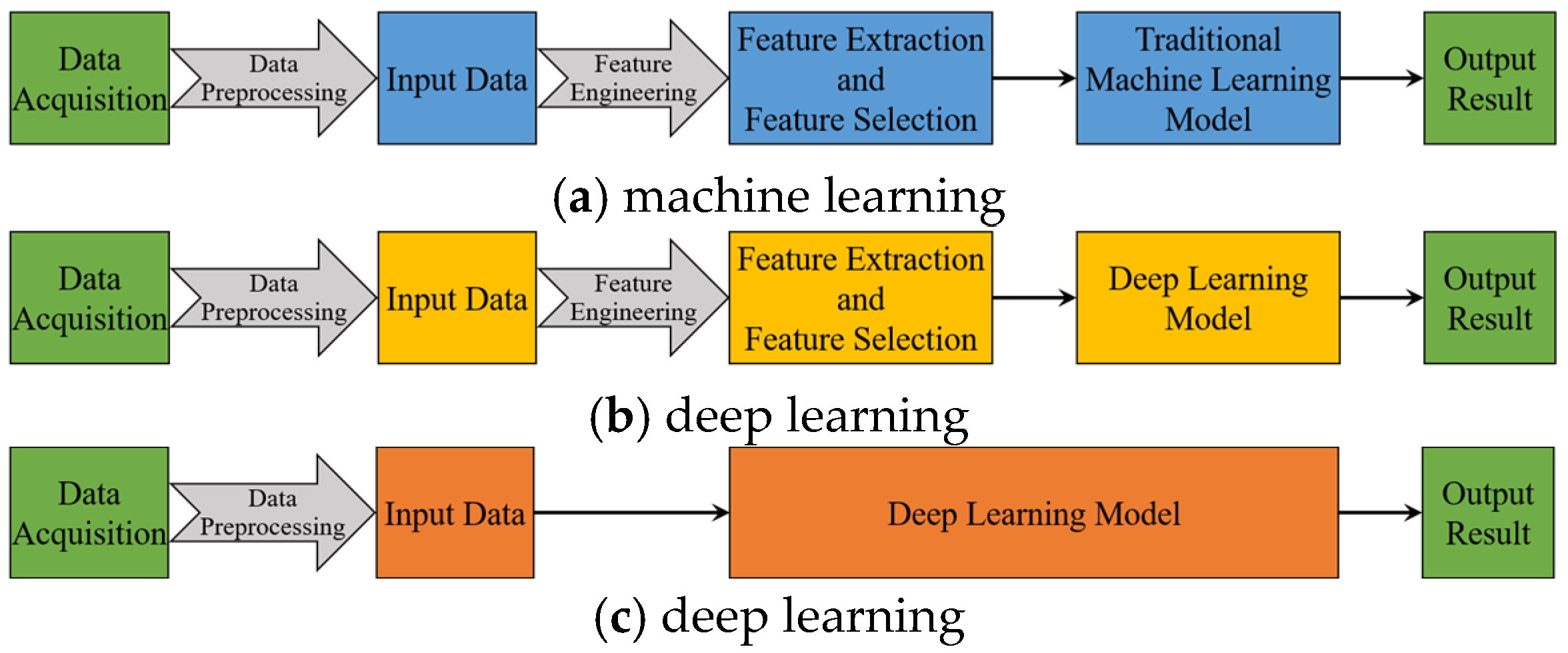
1. Introduction
2. Methodology of Input Paradigm and Time Series Presentation
2.1. Problem Description
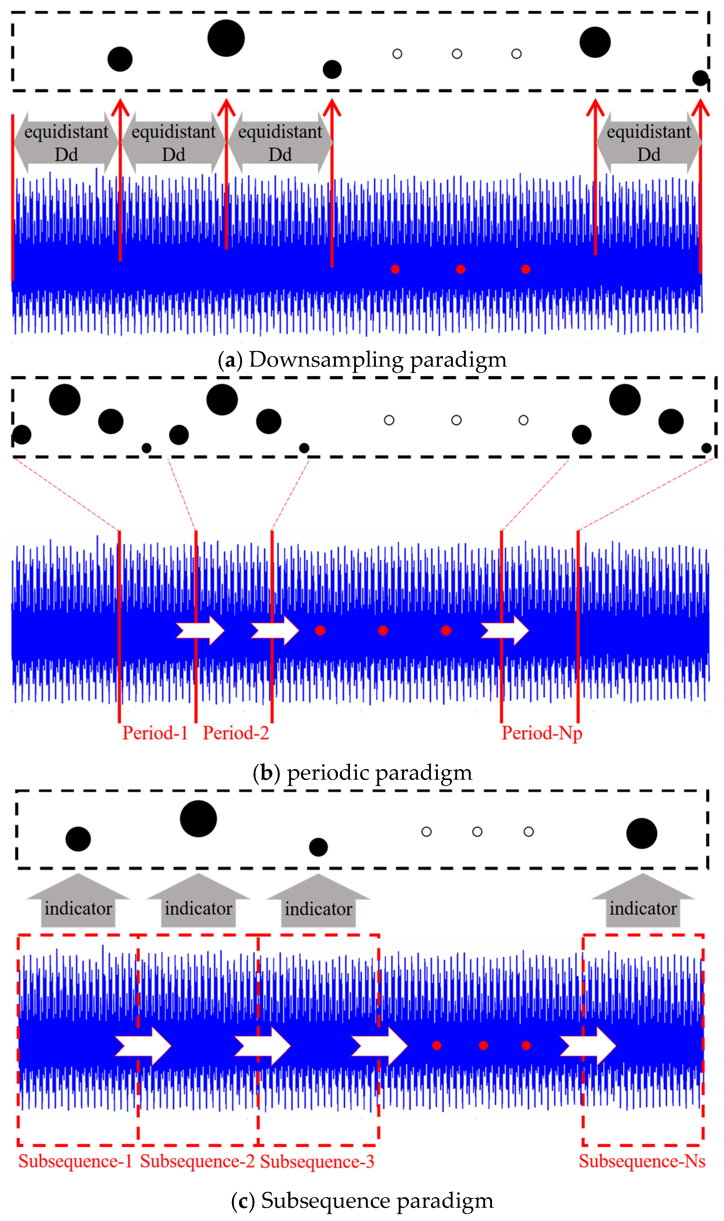
2.2. Design of Different Input Paradigms
2.2.1. Downsampling Paradigm
2.2.2. Periodic Paradigm
2.2.3. Subsequence Paradigm
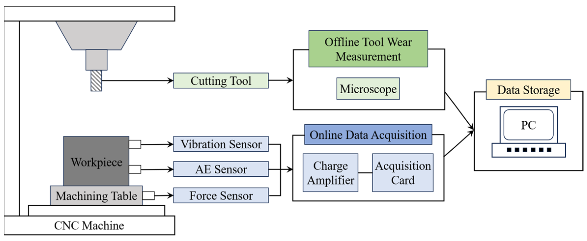
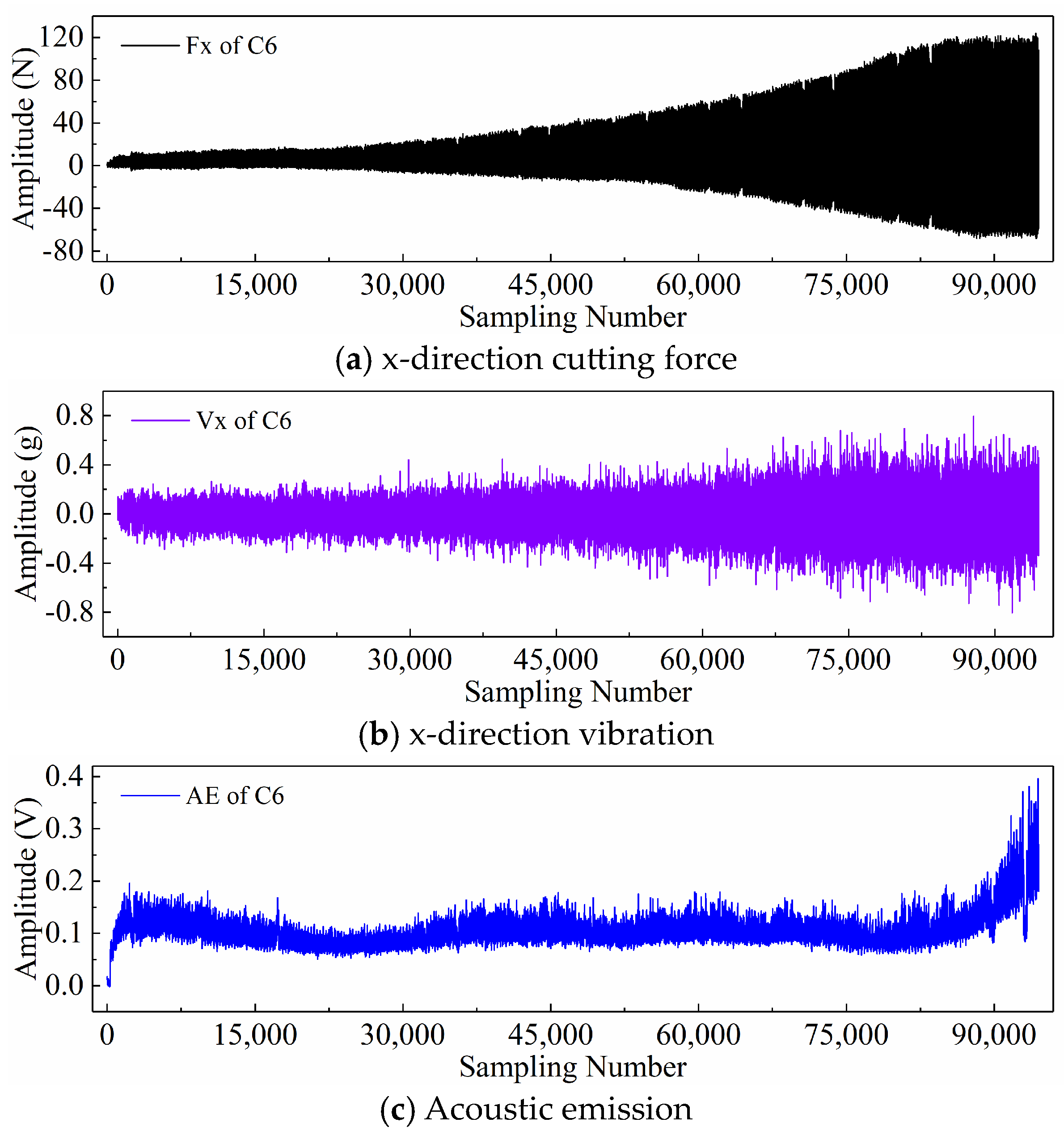
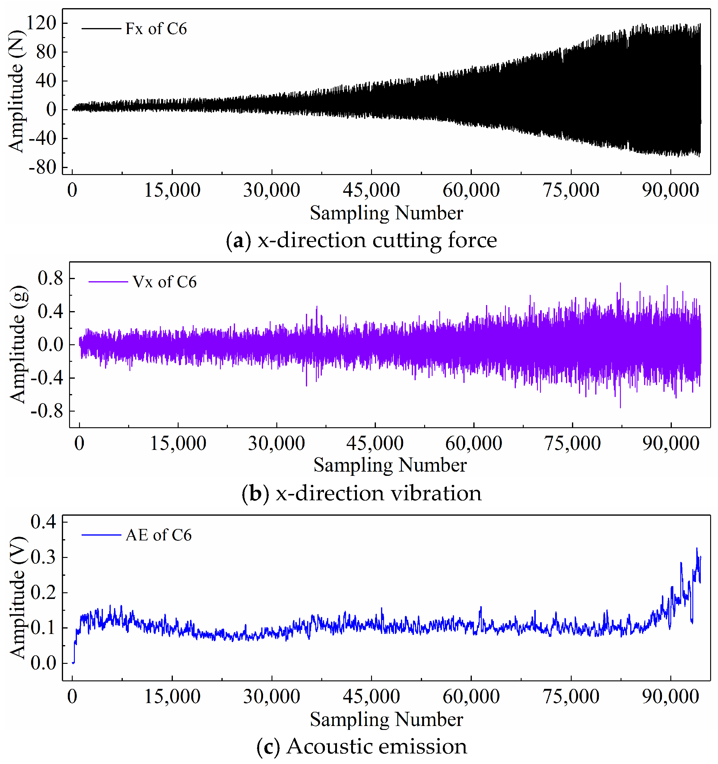
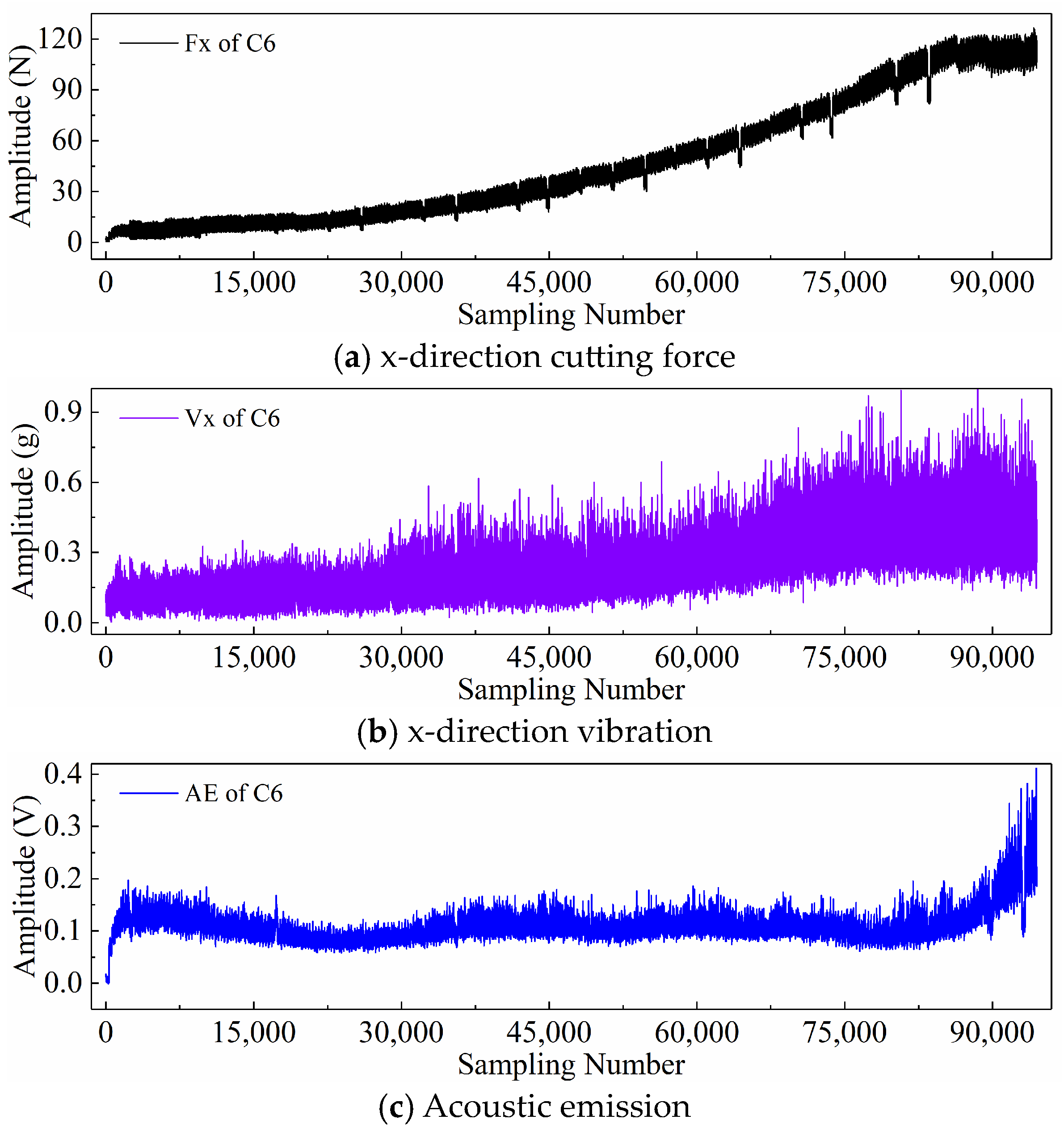
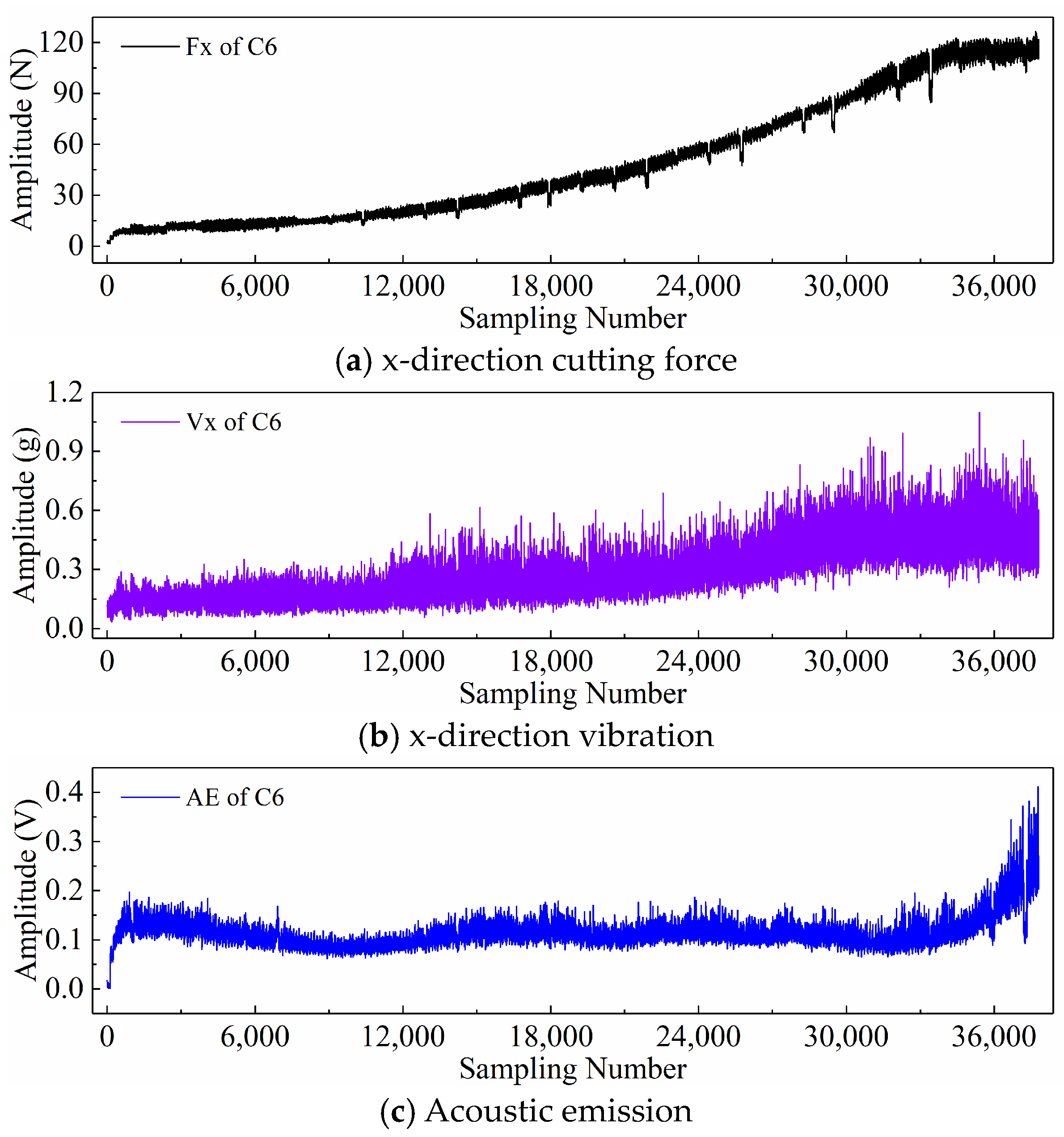
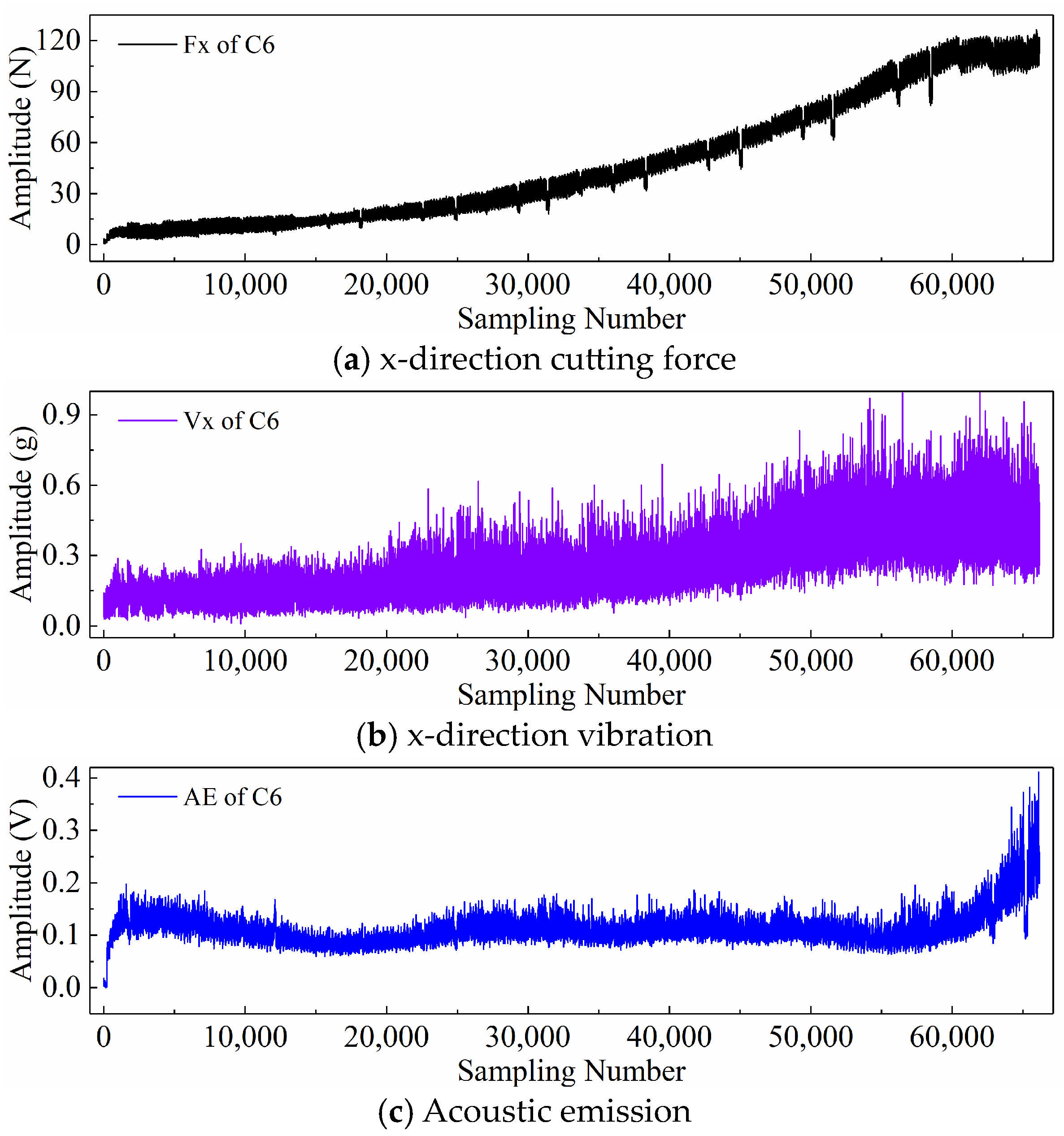
2.3. PHM2010 Dataset Description
2.4. Display of Time Series Generated by Different Input Paradigms
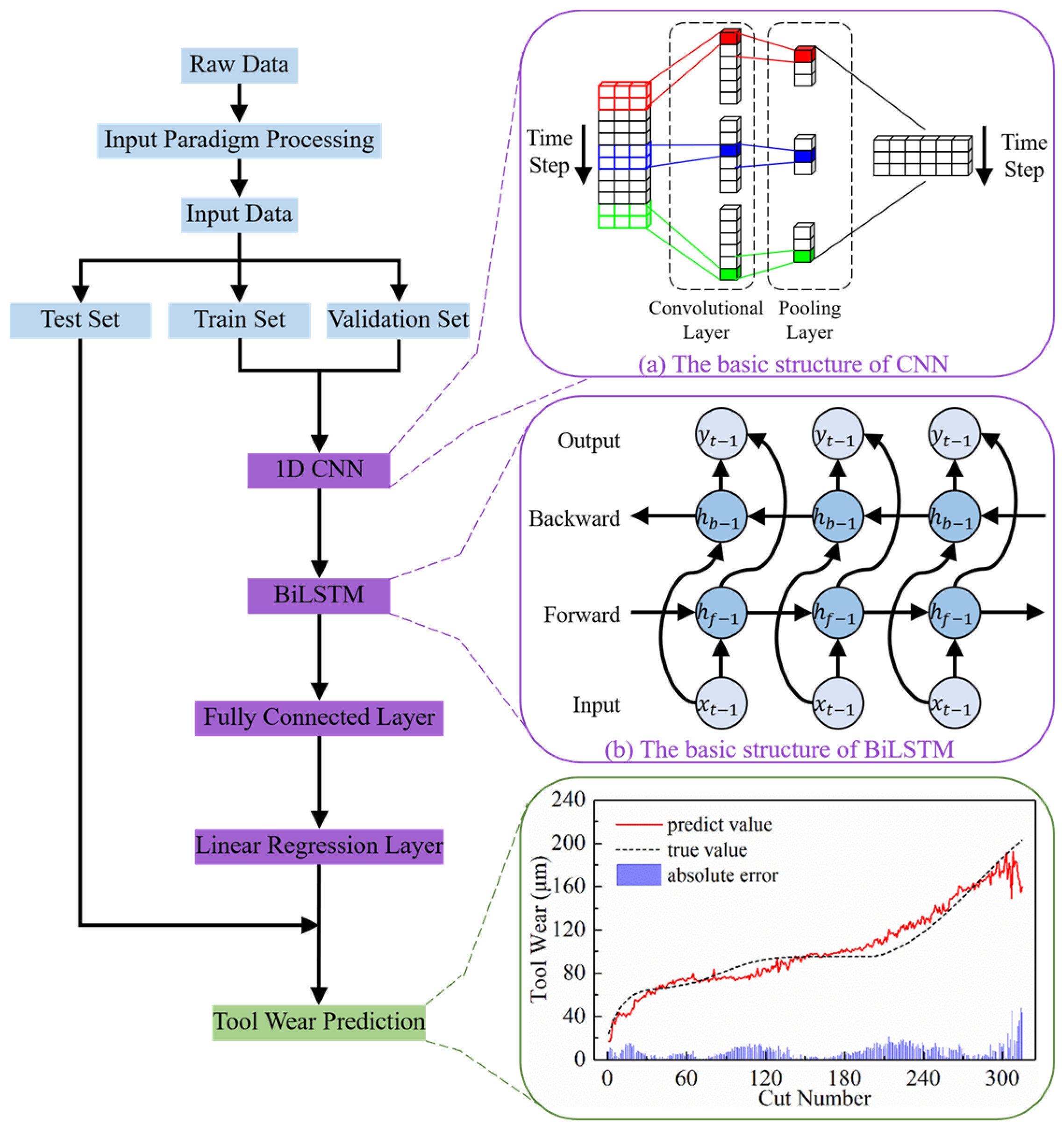
3. TCM Method Based on an Improved CNN-BiLSTM Hybrid Model
3.1. Model Architecture
3.1.1. CNN
3.1.2. BiLSTM
3.2. Model Training and Testing
3.2.1. Data Preprocessing
3.2.2. Implementation Details
4. Results and Discussion
4.1. Exploration of Different Input Paradigms
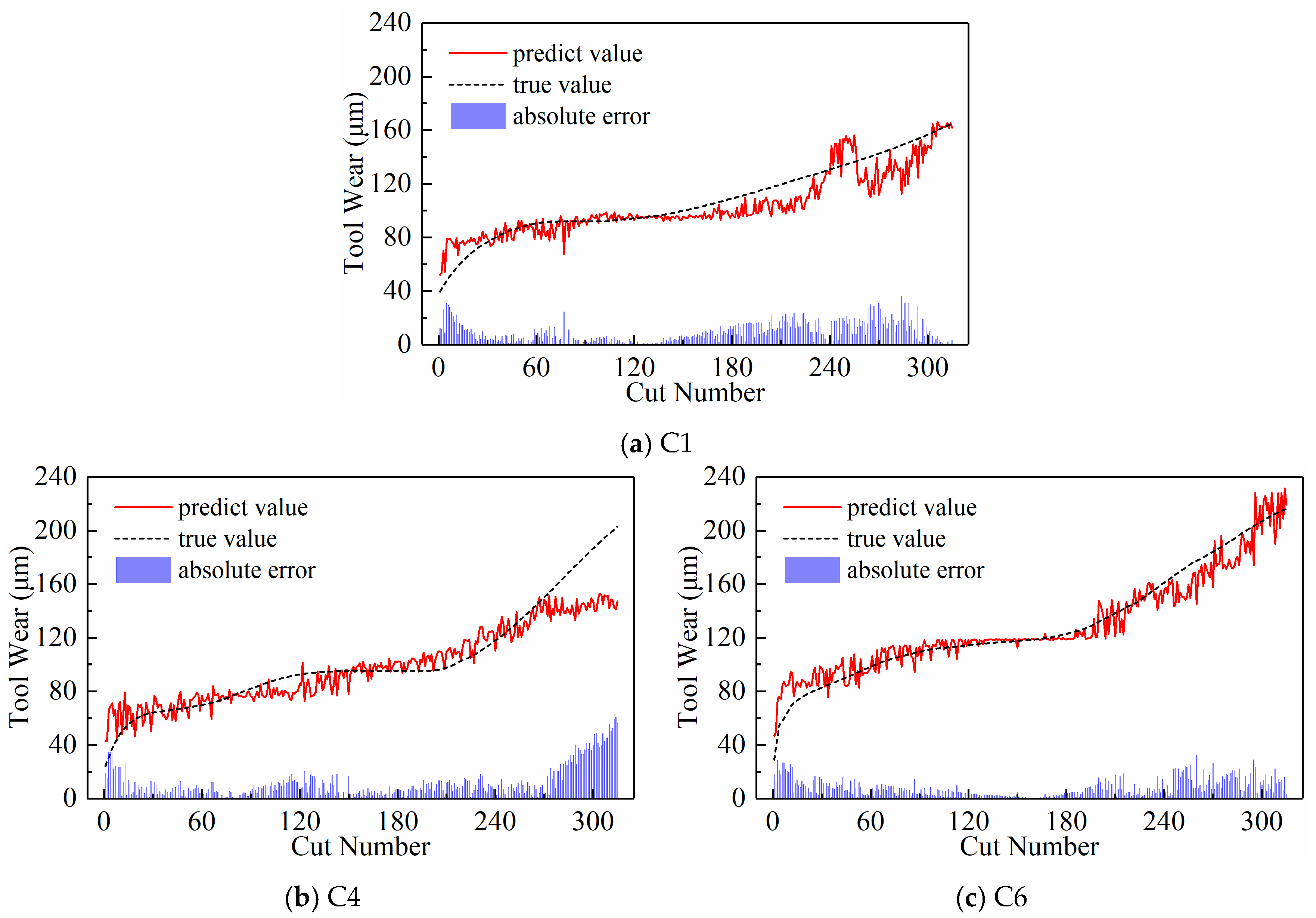
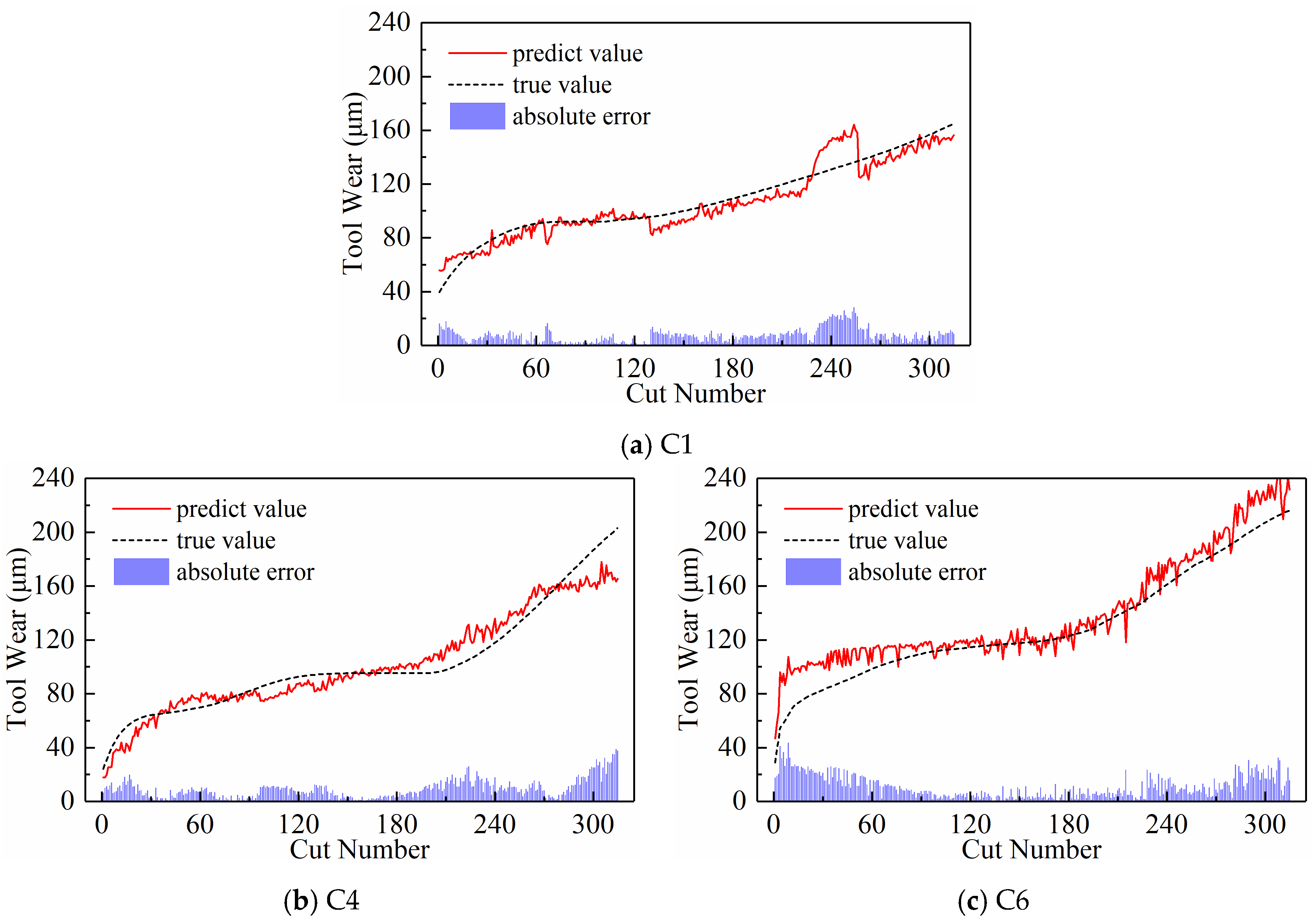
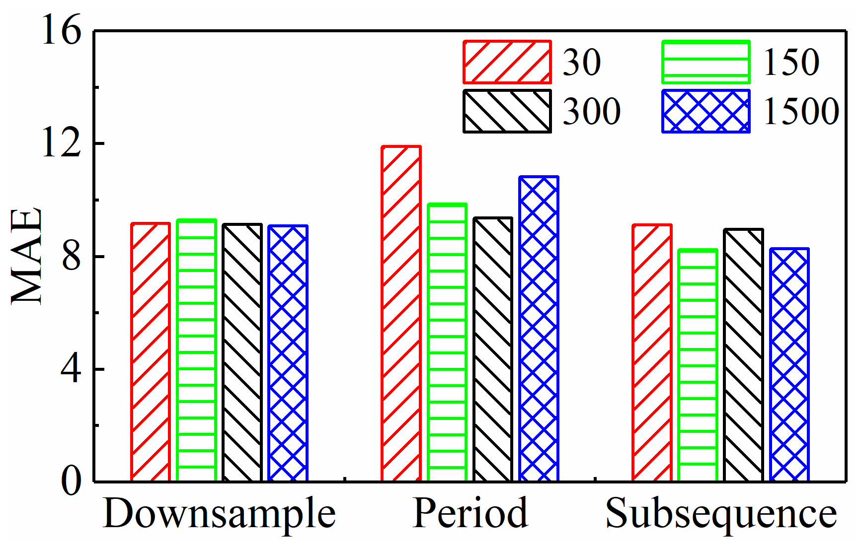
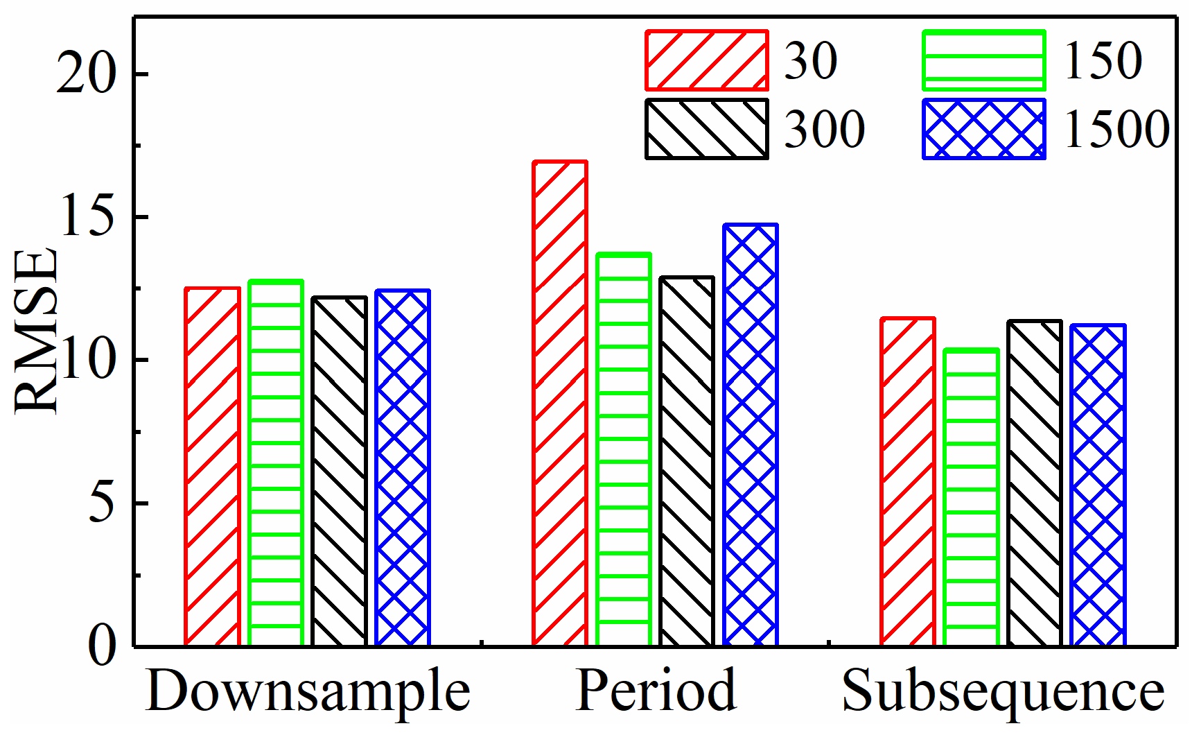
4.1.1. Model Performance of Different Input Paradigms
4.1.2. Dimensionality Reduction Potential of Different Input Paradigms
- Downsampling paradigm: Set intervals Nd to 1000, 200, 100, and 20, respectively.
- Periodic paradigm: Set the number of cycles Np to 0.1, 0.5, 1, and 5, respectively.
- Subsequence paradigm: Set the number of subsequences Ns to 30, 150, 300, and 1500, respectively.
4.2. Further Exploration of the Subsequence Paradigm
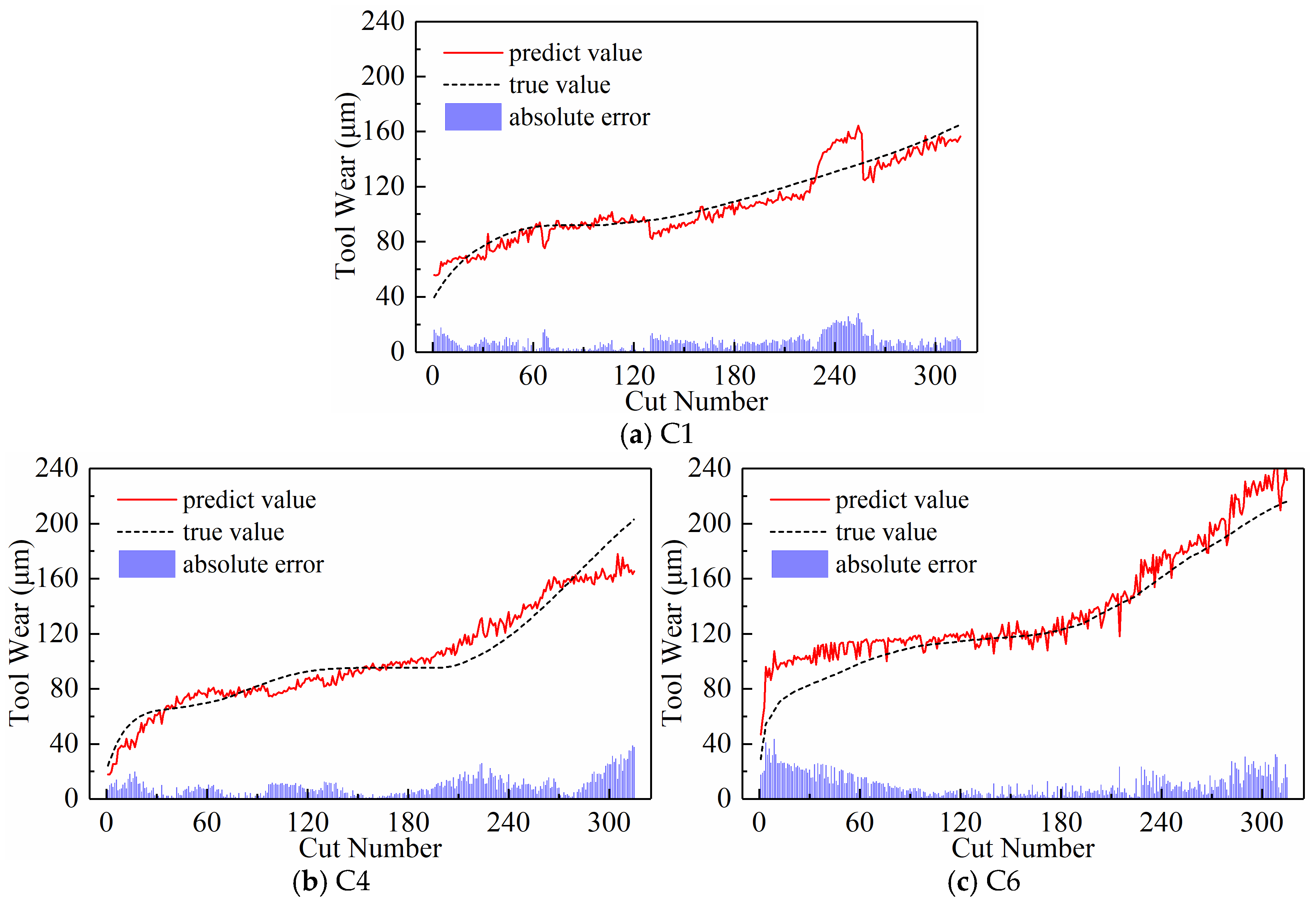
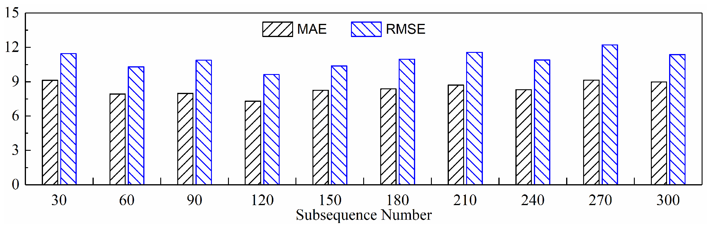
4.2.1. The Impact of Different Numbers of Subsequences on Model Performance
- (1)
- Display of Newly Generated Time Series
- (2)
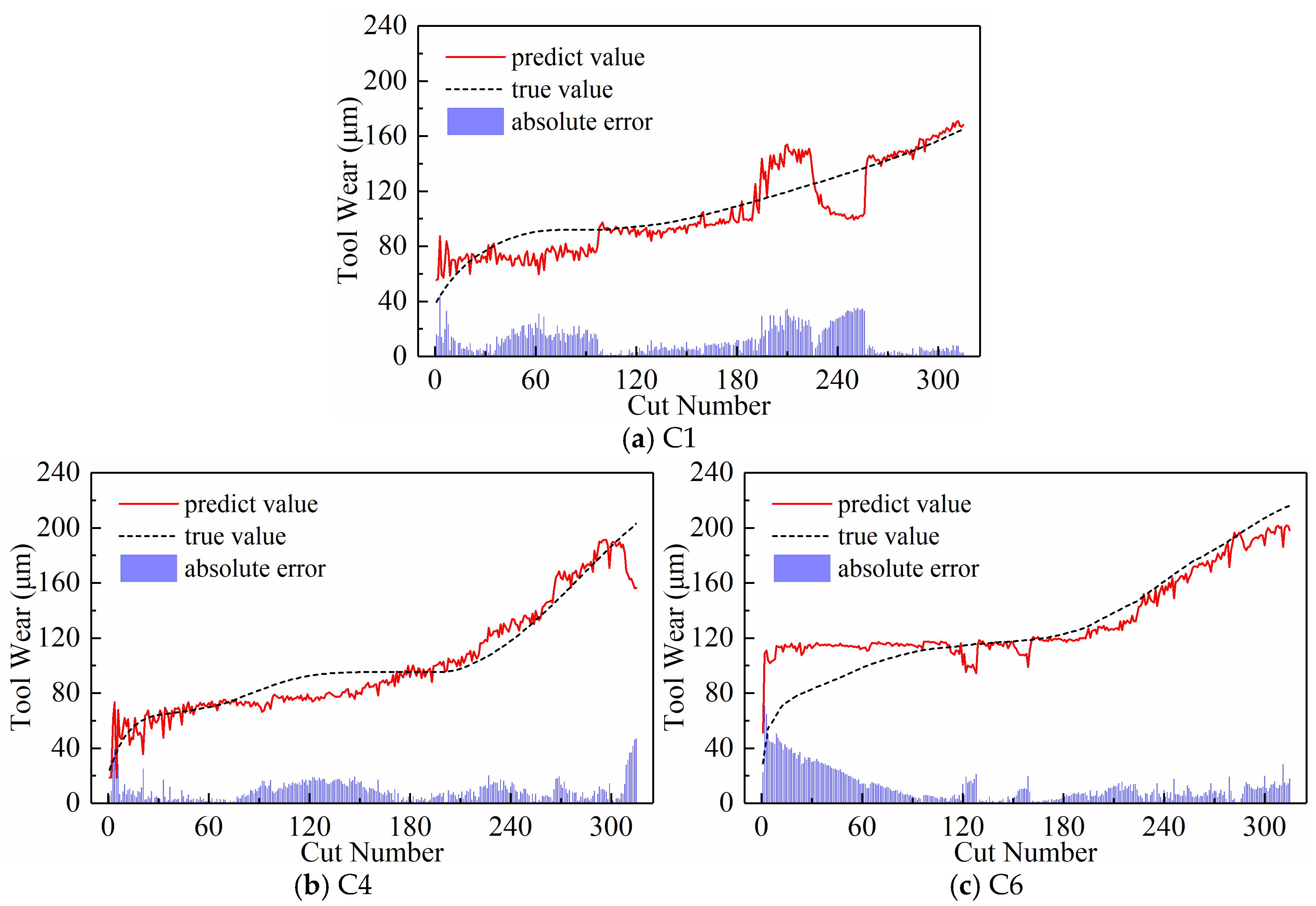
- Predictive Performance
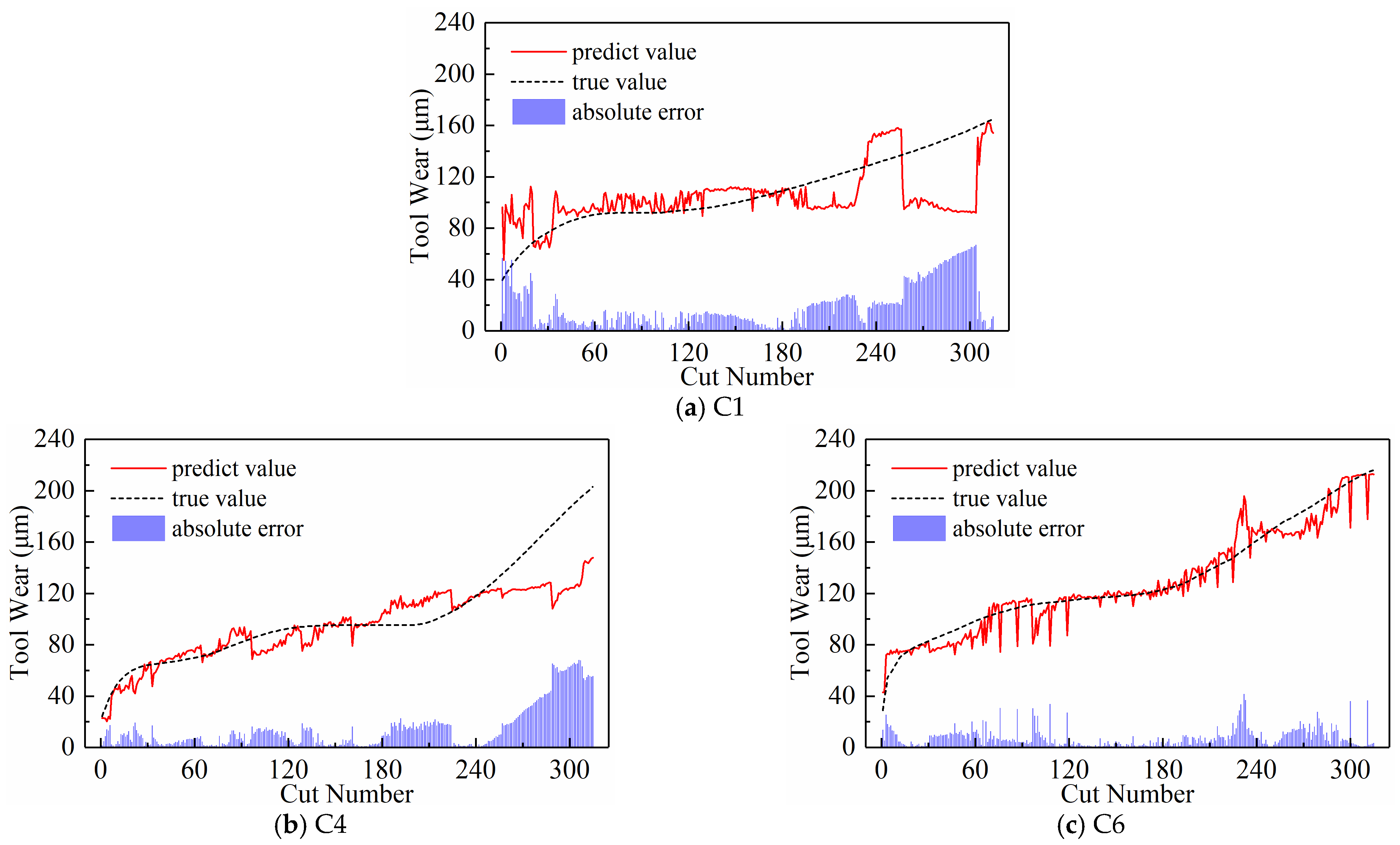
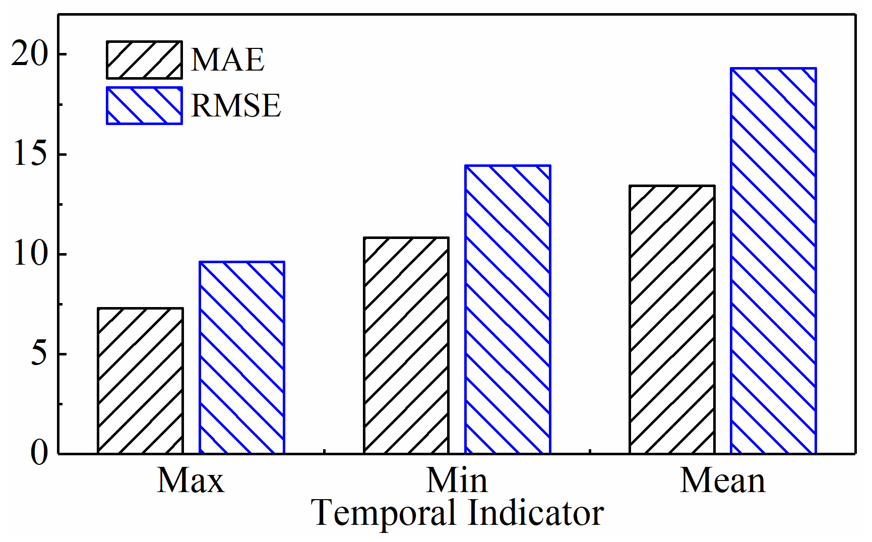
4.2.2. Impact of Different Temporal Indicators on Model Performance
- (1)
- Display of Newly Generated Time Series
- (2)
- Predictive Performance
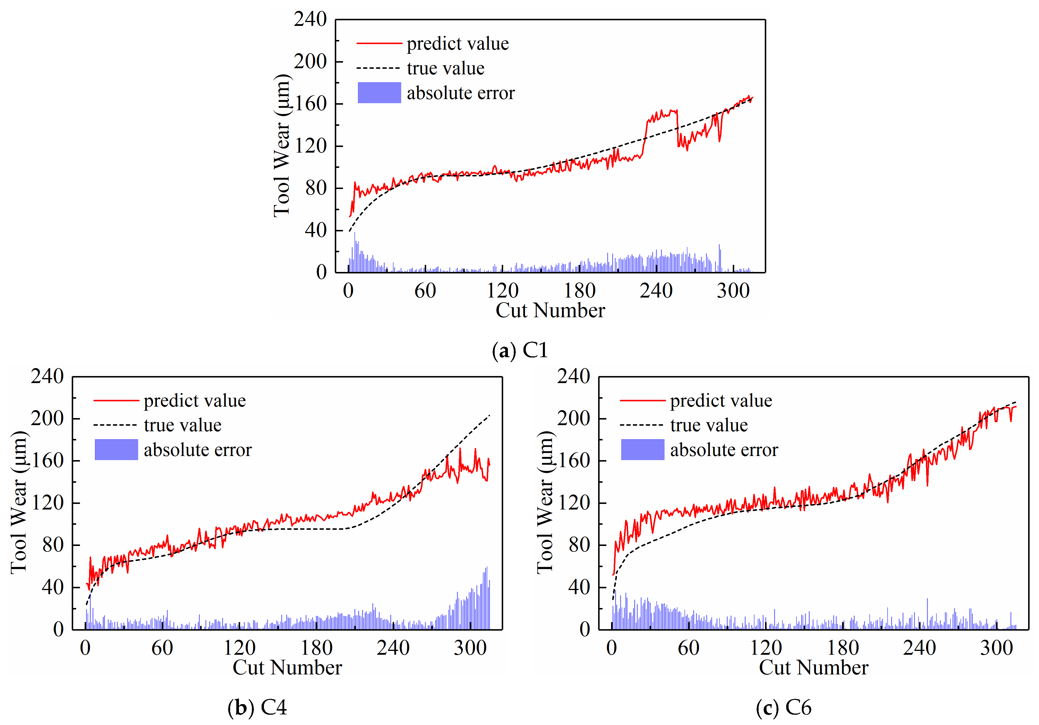
4.3. Comparison with Other Methods
5. Conclusions and Future Works
- (1)
- A new end-to-end framework for tool wear prediction was designed. Firstly, a suitable input paradigm was selected to generate new time series data directly into the model, eliminating the need for complex manual feature extraction. Then an improved CNN-BiLSTM hybrid model was utilized for prediction, capable of capturing the complex spatiotemporal correlation between the multi-sensor data and tool wear.
- (2)
- The subsequence paradigm had the lowest overall MAE and RMSE prediction performance metrics and the shortest computation time compared to the downsampling paradigm and the periodic paradigm. This shows that the subsequence paradigm is a great way to make TCM more effective and faster.
- (3)
- Further in-depth exploration of the subsequence paradigm revealed that the model’s MAE and RMSE were lowest when there were 120 subsequences and the temporal indicator was set to its highest value. This was after threefold cross-validation.
- (4)
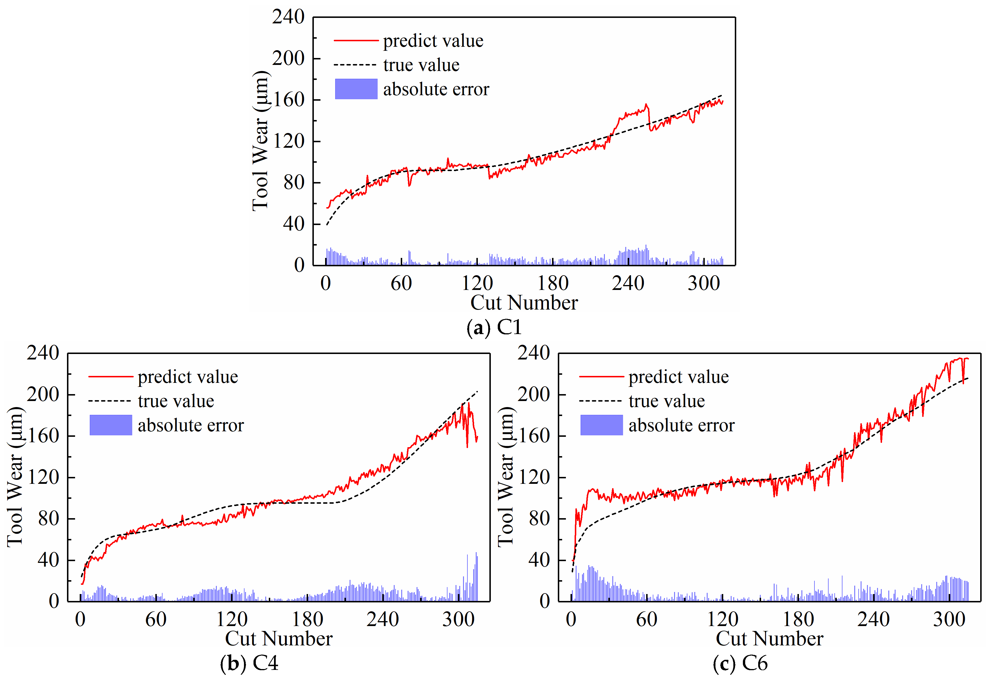
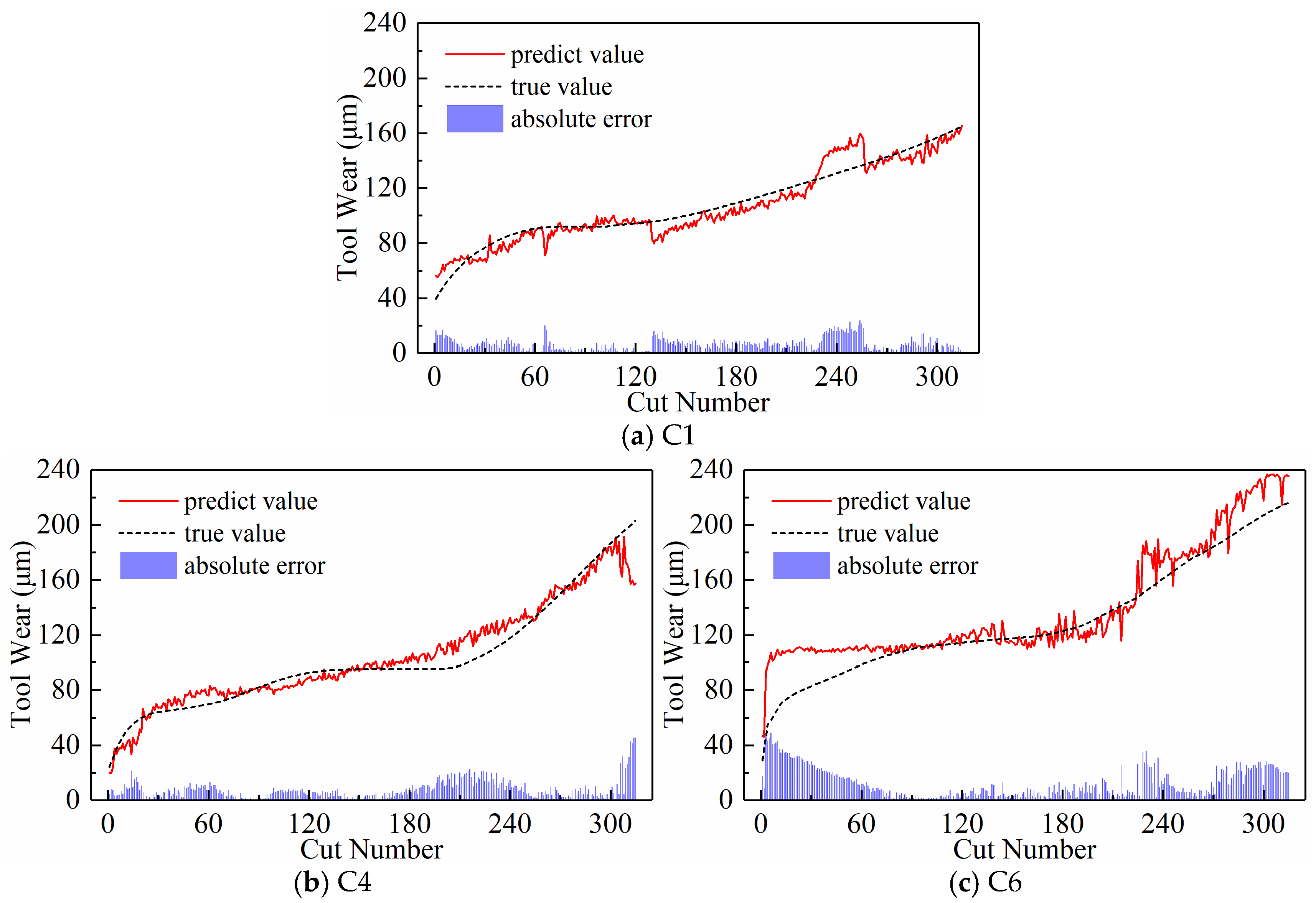
- Finally, we demonstrated the superiority of the proposed method by ditching feature engineering, overcoming the limitations of a single model architecture, and constructing high-quality input data by comparing the prediction performance of several classical and contemporary methods using the same dataset.
Author Contributions
Funding
Institutional Review Board Statement
Informed Consent Statement
Data Availability Statement
Conflicts of Interest
References
- Patil, S.S.; Pardeshi, S.S.; Patange, A.D.; Jegadeeshwaran, R. Deep learning algorithms for tool condition monitoring in milling: A review. Int. J. Phys. 2021, 1969, 012039. [Google Scholar] [CrossRef]
- Munaro, R.; Attanasio, A.; Del Prete, A. Tool Wear Monitoring with Artificial Intelligence Methods: A Review. J. Manuf. Mater. Proc. 2023, 7, 129. [Google Scholar] [CrossRef]
- Duan, J.; Zhang, X.; Shi, T. A hybrid attention-based paralleled deep learning model for tool wear prediction. Expert Syst. Appl. 2023, 211, 118548. [Google Scholar] [CrossRef]
- Serin, G.; Sener, B.; Ozbayoglu, A.M.; Unver, H.O. Review of tool condition monitoring in machining and opportunities for deep learning. Int. J. Adv. Manuf. Technol. 2020, 109, 953–974. [Google Scholar] [CrossRef]
- Cai, W.; Zhang, W.; Hu, X.; Liu, Y. A hybrid information model based on long short-term memory network for tool condition monitoring. J. Intell. Manuf. 2020, 31, 1497–1510. [Google Scholar] [CrossRef]
- Chen, Q.; Xie, Q.; Yuan, Q.; Huang, H.; Li, Y. Research on a real-time monitoring method for the wear state of a tool based on a convolutional bidirectional LSTM model. Symmetry 2019, 11, 1233. [Google Scholar] [CrossRef]
- Stavropoulos, P.; Papacharalampopoulos, A.; Souflas, T. Indirect online tool wear monitoring and model-based identification of process-related signal. Adv. Mech. Eng. 2020, 12, 1687814020919209. [Google Scholar] [CrossRef]
- Li, W.; Fu, H.; Han, Z.; Zhang, X.; Jin, H. Intelligent tool wear prediction based on Informer encoder and stacked bidirectional gated recurrent unit. Robot. Comput. Integr. Manuf. 2022, 77, 102368. [Google Scholar] [CrossRef]
- Shokrani, A.; Dogan, H.; Burian, D.; Nwabueze, T.D.; Kolar, P.; Liao, Z.; Sadek, A.; Teti, R.; Wang, P.; Pavel, R.; et al. Sensors for in-process and on-machine monitoring of machining operations. CIRP J. Manuf. Sci. Technol. 2024, 51, 263–292. [Google Scholar] [CrossRef]
- Li, K.; Qiu, C.; Zhou, X.; Chen, M.; Lin, Y.; Jia, X.; Li, B. Modeling and tagging of time sequence signals in the milling process based on an improved hidden semi-Markov model. Expert. Syst. Appl. 2022, 205, 117758. [Google Scholar] [CrossRef]
- Twardowski, P.; Tabaszewski, M.; Wiciak–Pikuła, M.; Felusiak-Czyryca, A. Identification of tool wear using acoustic emission signal and machine learning methods. Precis. Eng. 2021, 72, 738–744. [Google Scholar] [CrossRef]
- Zhang, K.; Zhu, H.; Liu, D.; Wang, G.; Huang, C.; Yao, P. A dual compensation strategy based on multi-model support vector regression for tool wear monitoring. Meas. Sci. Technol. 2022, 33, 105601. [Google Scholar] [CrossRef]
- Pratap, A.; Patra, K.; Joshi, S.S. Identification of tool life stages and redressing criterion for PCD micro-grinding tools using a machine learning approach. J. Manuf. Sci. Eng. 2022, 145, 1–29. [Google Scholar]
- Gai, X.; Cheng, Y.; Guan, R.; Jin, Y.; Lu, M. Tool wear state recognition based on WOA-SVM with statistical feature fusion of multi-signal singularity. Int. J. Adv. Manuf. Technol. 2022, 123, 2209–2225. [Google Scholar] [CrossRef]
- Babu, M.S.; Rao, T.B. Multi-sensor heterogeneous data-based online tool health monitoring in milling of IN718 superalloy using OGM (1, N) model and SVM. Measurement 2022, 199, 111501. [Google Scholar] [CrossRef]
- Cheng, Y.N.; Jin, Y.B.; Gai, X.Y.; Guan, R.; Lu, M.D. Prediction of tool wear in milling process based on BP neural network optimized by firefly algorithm. Proc. Inst. Mech. Eng. E J. Process Mech. Eng. 2023. [Google Scholar] [CrossRef]
- Gomes, M.C.; Brito, L.C.; da Silva, M.B.; Duarte, M.A.V. Tool wear monitoring in micromilling using support vector machine with vibration and sound sensors. Precis. Eng. 2021, 67, 137–151. [Google Scholar] [CrossRef]
- Li, K.M.; Lin, Y.Y. Tool wear classification in milling for varied cutting conditions: With emphasis on data pre-processing. Int. J. Adv. Manuf. Technol. 2023, 125, 341–355. [Google Scholar] [CrossRef]
- Dhobale, N.; Mulik, S.S.; Deshmukh, S.P. Naïve Bayes and Bayes net classifier for fault diagnosis of end mill tool using wavelet analysis: A comparative study. J. Vib. Eng. Technol. 2022, 10, 1721–1735. [Google Scholar] [CrossRef]
- Papacharalampopoulos, A.; Alexopoulos, K.; Catti, P.; Stavropoulos, P.; Chryssolouris, G. Learning More with Less Data in Manufacturing: The Case of Turning Tool Wear Assessment through Active and Transfer Learning. Processes 2024, 12, 1262. [Google Scholar] [CrossRef]
- Zhao, R.; Yan, R.; Wang, J.; Mao, K. Learning to Monitor Machine Health with Convolutional Bi-Directional LSTM Networks. Sensors 2017, 17, 273. [Google Scholar] [CrossRef]
- Ranawat, N.S.; Prakash, J.; Miglani, A.; Kankar, P.K. Performance evaluation of LSTM and Bi-LSTM using non-convolutional features for blockage detection in centrifugal pump. Eng. Appl. Artif. Intell. 2023, 122, 106092. [Google Scholar] [CrossRef]
- Hinton, G.; Salakhutdinov, R.R. Reducing the dimensionality of data with neural networks. Science 2006, 313, 504–507. [Google Scholar] [CrossRef]
- Gao, K.; Xu, X.; Jiao, S. Measurement and prediction of wear volume of the tool in nonlinear degradation process based on multi-sensor information fusion. Eng. Fail. Anal. 2022, 136, 106164. [Google Scholar] [CrossRef]
- Aghazadeh, F.; Tahan, A.; Thomas, M. Tool condition monitoring using spectral subtraction and convolutional neural networks in milling process. Int. J. Adv. Manuf. Technol. 2018, 98, 3217–3227. [Google Scholar] [CrossRef]
- Zhao, R.; Yan, R.; Chen, Z.; Mao, K.; Wang, P.; Gao, R.X. Deep learning and its applications to machine health monitoring. Mech. Syst. Signal Process. 2019, 115, 213–237. [Google Scholar] [CrossRef]
- Hall, S.; Newman, S.T.; Loukaides, E.; Shokrani, A. ConvLSTM deep learning signal prediction for forecasting bending moment for tool condition monitoring. Procedia CIRP 2022, 107, 1071–1076. [Google Scholar] [CrossRef]
- Gudelek, M.U.; Serin, G.; Ozbayoglu, A.M.; Unver, H.O. An industrially viable wavelet long-short term memory-deep multilayer perceptron-based approach to tool condition monitoring considering operational variability. Proc. Inst. Mech. Eng. Part E J. Process Mech. Eng. 2023, 237, 2532–2546. [Google Scholar] [CrossRef]
- Ma, K.; Wang, G.; Yang, K.; Hu, M.; Li, J. Tool wear monitoring for cavity milling based on vibration singularity analysis and stacked LSTM. Int. J. Adv. Manuf. Technol. 2022, 120, 4023–4039. [Google Scholar] [CrossRef]
- Wickramarachchi, C.T.; Rogers, T.J.; McLeay, T.E.; Leahy, W.; Cross, E.J. Online damage detection of cutting tools using Dirichlet process mixture models. Mech. Syst. Signal Process. 2022, 180, 109434. [Google Scholar] [CrossRef]
- Ahmed, M.; Kamal, K.; Ratlamwala, T.A.; Hussain, G.; Alqahtani, M.; Alkahtani, M.; Alatefi, M.; Alzabidi, A. Tool health monitoring of a milling process using acoustic emissions and a ResNet deep learning model. Sensors 2023, 23, 3084. [Google Scholar] [CrossRef]
- Hassan, M.; Sadek, A.; Attia, H. A Real-Time Deep Machine Learning Approach for Sudden Tool Failure Prediction and Prevention in Machining Processes. Sensors 2023, 23, 3894. [Google Scholar] [CrossRef] [PubMed]
- Shah, M.; Vakharia, V.; Chaudhari, R.; Vora, J.; Pimenov, D.Y.; Giasin, K. Tool wear prediction in face milling of stainless steel using singular generative adversarial network and LSTM deep learning models. Int. J. Adv. Manuf. Technol. 2022, 121, 723–736. [Google Scholar] [CrossRef]
- Liu, C.; Zhu, L. A two-stage approach for predicting the remaining useful life of tools using bidirectional long short-term memory. Measurement 2020, 164, 108029. [Google Scholar] [CrossRef]
- De Barrena, T.F.; Ferrando, J.L.; García, A.; Badiola, X.; de Buruaga, M.S.; Vicente, J. Tool remaining useful life prediction using bidirectional recurrent neural networks (BRNN). Int. J. Adv. Manuf. Technol. 2023, 125, 4027–4045. [Google Scholar] [CrossRef]
- Huang, Z.; Zhu, J.; Lei, J.; Li, X.; Tian, F. Tool wear predicting based on multi-domain feature fusion by deep convolutional neural network in milling operations. J. Intell. Manuf. 2020, 31, 953–966. [Google Scholar] [CrossRef]
- Bazi, R.; Benkedjouh, T.; Habbouche, H.; Rechak, S.; Zerhouni, N. A hybrid CNN-BiLSTM approach-based variational mode decomposition for tool wear monitoring. Int. J. Adv. Manuf. Technol. 2022, 119, 3803–3817. [Google Scholar] [CrossRef]
- Zhang, X.; Lu, X.; Li, W.; Wang, S. Prediction of the remaining useful life of cutting tool using the Hurst exponent and CNN-LSTM. Int. J. Adv. Manuf. Technol. 2021, 112, 2277–2299. [Google Scholar] [CrossRef]
- Sayyad, S.; Kumar, S.; Bongale, A.; Kotecha, K.; Selvachandran, G.; Suganthan, P.N. Tool wear prediction using long short-term memory variants and hybrid feature selection techniques. Int. J. Adv. Manuf. Tech. 2022, 121, 6611–6633. [Google Scholar] [CrossRef]
- Wang, C.Y.; Huang, C.Y.; Chiang, Y.H. Solutions of feature and Hyperparameter model selection in the intelligent manufacturing. Processes 2022, 10, 862. [Google Scholar] [CrossRef]
- Li, X.; Liu, X.; Yue, C.; Wang, L.; Liang, S.Y. Data-model linkage prediction of tool remaining useful life based on deep feature fusion and Wiener process. J. Manuf. Syst. 2024, 73, 19–38. [Google Scholar] [CrossRef]
- Liu, X.; Liu, S.; Li, X.; Zhang, B.; Yue, C.; Liang, S.Y. Intelligent tool wear monitoring based on parallel residual and stacked bidirectional long short-term memory network. J. Manuf. Syst. 2021, 60, 608–619. [Google Scholar] [CrossRef]
- Arias, V.A.; Vargas-Machuca, J.; Zegarra, F.C.; Coronado, A.M. Convolutional Neural Network Classification for Machine Tool Wear Based on Unsupervised Gaussian Mixture Model. In Proceedings of the 2021 IEEE Sciences and Humanities International Research Conference (SHIRCON), Lima, Peru, 17–19 November 2021; pp. 1–4. [Google Scholar]
- Zhang, N.; Chen, E.; Wu, Y.; Guo, B.; Jiang, Z.; Wu, F. A novel hybrid model integrating residual structure and bi-directional long short-term memory network for tool wear monitoring. Int. J. Adv. Manuf. Technol. 2022, 120, 6707–6722. [Google Scholar] [CrossRef]
- Suawa, P.F.; Hübner, M. Health monitoring of milling tools under distinct operating conditions by a deep convolutional neural network model. In Proceedings of the 2022 Design, Automation & Test in Europe Conference & Exhibition (DATE), Antwerp, Belgium, 14–23 March 2022; pp. 1107–1110. [Google Scholar]
- Chao, K.C.; Shih, Y.; Lee, C.H. A novel sensor-based label-smoothing technique for machine state degradation. IEEE Sens. J. 2023, 23, 10879–10888. [Google Scholar] [CrossRef]
- Yang, J.; Wu, J.; Li, X.; Qin, X. Tool wear prediction based on parallel dual-channel adaptive feature fusion. Int. J. Adv. Manuf. Technol. 2023, 128, 145–165. [Google Scholar] [CrossRef]
- Caggiano, A.; Mattera, G.; Nele, L. Smart tool wear monitoring of CFRP/CFRP stack drilling using autoencoders and memory-based neural networks. Appl. Sci. 2023, 13, 3307. [Google Scholar] [CrossRef]
- Zhao, R.; Wang, J.; Yan, R.; Mao, K. Machine health monitoring with LSTM networks. In Proceedings of the 10th International Conference on Sensing Technology (ICST), Nanjing, China, 11–13 November 2016. [Google Scholar]
- Marani, M.; Zeinali, M.; Songmene, V.; Mechefske, C.K. Tool wear prediction in high-speed turning of a steel alloy using long short-term memory modelling. Measurement 2021, 177, 109329. [Google Scholar] [CrossRef]
- Kim, G.; Yang, S.M.; Kim, D.M.; Kim, S.; Choi, J.G.; Ku, M.; Lim, S.; Park, H.W. Bayesian-based uncertainty-aware tool-wear prediction model in end-milling process of titanium alloy. Appl. Soft Comput. 2023, 148, 110922. [Google Scholar] [CrossRef]
- Jeon, W.S.; Rhee, S.Y. Tool Wear Monitoring System Using Seq2Seq. Machines 2024, 12, 169. [Google Scholar] [CrossRef]
- Yin, Y.; Wang, S.; Zhou, J. Multisensor-based tool wear diagnosis using 1D-CNN and DGCCA. Appl. Intell. 2023, 53, 4448–4461. [Google Scholar] [CrossRef]
- Chan, Y.W.; Kang, T.C.; Yang, C.T.; Chang, C.H.; Huang, S.M.; Tsai, Y.T. Tool wear prediction using convolutional bidirectional LSTM networks. J. Supercomput. 2022, 78, 810–832. [Google Scholar] [CrossRef]
- Nie, L.; Zhang, L.; Xu, S.; Cai, W.; Yang, H. Remaining useful life prediction of milling cutters based on CNN-BiLSTM and attention mechanism. Symmetry 2022, 14, 2243. [Google Scholar] [CrossRef]
- Ma, L.; Zhang, N.; Zhao, J.; Kong, H. An end-to-end deep learning approach for tool wear condition monitoring. Int. J. Adv. Manuf. Technol. 2024, 133, 2907–2920. [Google Scholar] [CrossRef]
- Wang, S.; Yu, Z.; Xu, G.; Zhao, F. Research on tool remaining life prediction method based on CNN-LSTM-PSO. IEEE Access 2023, 11, 80448–80464. [Google Scholar] [CrossRef]
- Li, Y.; Wang, X.; He, Y.; Wang, Y.; Wang, Y.; Wang, S. Deep spatial-temporal feature extraction and lightweight feature fusion for tool condition monitoring. IEEE Trans. Ind. Electron. 2021, 69, 7349–7359. [Google Scholar] [CrossRef]
- Zegarra, F.C.; Vargas-Machuca, J.; Coronado, A.M. Comparison of CNN and CNN-LSTM architectures for tool wear estimation. In Proceedings of the 2021 IEEE Engineering International Research Conference (EIRCON), Lima, Peru, 27–29 October 2021; pp. 1–4. [Google Scholar]
- Li, R.; Ye, X.; Yang, F.; Du, K.L. ConvLSTM-Att: An attention-based composite deep neural network for tool wear prediction. Machines 2023, 11, 297. [Google Scholar] [CrossRef]
- Justus, V.; Kanagachidambaresan, G.R. Machine learning based fault-oriented predictive maintenance in industry 4.0. Int. J. Syst. Assur. Eng. Manag. 2024, 15, 462–474. [Google Scholar] [CrossRef]
- Li, B.; Lu, Z.; Jin, X.; Zhao, L. Tool wear prediction in milling CFRP with different fiber orientations based on multi-channel 1DCNN-LSTM. J. Intell. Manuf. 2023, 35, 2547–2566. [Google Scholar] [CrossRef]
- Liu, X.; Zhang, B.; Li, X.; Liu, S.; Yue, C.; Liang, S.Y. An approach for tool wear prediction using customized DenseNet and GRU integrated model based on multi-sensor feature fusion. J. Intell. Manuf. 2023, 34, 885–902. [Google Scholar] [CrossRef]
- PHM Society. PHM Society Conference Data Challenge. 2010. Available online: https://data.phmsociety.org/2021-phm-conference-data-challenge/ (accessed on 30 May 2024).
- ISO 8688-2:1989(E); Tool Life Testing in Milling—Part 2: End milling. ISO: London, UK, 1989.
- Hochreiter, S.; Schmidhuber, J. Long short-term memory. Neural Comput. 1997, 9, 1735–1780. [Google Scholar] [CrossRef]
- Li, X.; Qin, X.; Wu, J.; Yang, J.; Huang, Z. Tool wear prediction based on convolutional bidirectional LSTM model with improved particle swarm optimization. Int. J. Adv. Manuf. Technol. 2022, 123, 4025–4039. [Google Scholar] [CrossRef]
- Qin, Y.; Liu, X.; Yue, C.; Zhao, M.; Wei, X.; Wang, L. Tool wear identification and prediction method based on stack sparse self-coding network. J. Manuf. Syst. 2023, 68, 72–84. [Google Scholar] [CrossRef]
- Wang, J.; Yan, J.; Li, C.; Gao, R.X.; Zhao, R. Deep heterogeneous GRU model for predictive analytics in smart manufacturing: Application to tool wear prediction. Comput. Ind. 2019, 111, 1–14. [Google Scholar] [CrossRef]
- Qiao, H.; Wang, T.; Wang, P.; Qiao, S.; Zhang, L. A time-distributed spatiotemporal feature learning method for machine health monitoring with multi-sensor time series. Sensors 2018, 18, 2932. [Google Scholar] [CrossRef]


| Milling Parameters | Value | Equipment Type | Equipment Model |
|---|---|---|---|
| Milling method | Climb milling | Machine | Roders RFM760 (Roders, Soltau, Germany) |
| Cooling method | Dry cutting | Tool | Ball-end carbide milling cutter (Roders, Soltau, Germany) |
| Spindle speed (r/min) | 10,400 | Workpiece material | Stainless steel HRC52 |
| Feed rate (mm/min) | 1555 | Vibration sensor | Kistler 8636C acceleration sensor (Kistler, Winterthur, Swiss) |
| Tool feeding amount (mm) | 0.001 | AE sensor | Kistler 8152 acoustic emission sensor (Kistler, Winterthur, Swiss) |
| Cutting width (mm) | 0.125 | Force sensor | Kistler 9265B dynamometer (Kistler, Winterthur, Swiss) |
| Cutting depth (mm) | 0.2 | Data acquisition card | DAQ NI PCI 1200 (National Instruments, Austin, TX, USA) |
| Cutting length (mm) | 108 | Charge amplifier | Kistler charge amplifier (Kistler, Winterthur, Swiss) |
| Sampling frequency (kHz) | 50 | Microscope | LEICA MZ12 microscope (Leica, Solms, Germany) |
| Parameter | Learning Rate | Batch Size | Dropout Rate | Epoch | Optimizer | Activation |
|---|---|---|---|---|---|---|
| Value | 0.001 | 128 | 0.2 | 500 (early stopping) | Adam | ReLU |
| Input Paradigms | Test Data | Computational Time (s) | |||||
|---|---|---|---|---|---|---|---|
| C1 | C4 | C6 | |||||
| MAE | RMSE | MAE | RMSE | MAE | RMSE | ||
| downsampling-100 | 7.49 | 9.99 | 10.66 | 14.56 | 9.26 | 11.96 | 93.26 |
| periodic-1 | 9.03 | 11.87 | 11.30 | 16.53 | 7.76 | 10.33 | 108.12 |
| subsequence-300 | 7.10 | 8.92 | 8.92 | 11.39 | 10.88 | 13.78 | 76.89 |
| Input Paradigms | Input Sequence Length | Test Set | |||||
|---|---|---|---|---|---|---|---|
| C1 | C4 | C6 | |||||
| MAE | RMSE | MAE | RMSE | MAE | RMSE | ||
| Downsampling paradigm | 30 | 9.18 | 11.87 | 11.33 | 16.44 | 7.00 | 9.25 |
| 150 | 6.73 | 8.95 | 10.59 | 15.92 | 10.57 | 13.46 | |
| 300 | 7.49 | 9.99 | 10.66 | 14.56 | 9.26 | 11.96 | |
| 1500 | 8.40 | 10.59 | 9.81 | 14.85 | 9.02 | 11.81 | |
| Periodic paradigm | 30 | 9.94 | 13.89 | 13.54 | 20.17 | 12.24 | 16.76 |
| 150 | 9.50 | 12.45 | 11.33 | 16.67 | 8.72 | 12.05 | |
| 300 | 9.03 | 11.87 | 11.30 | 16.53 | 7.76 | 10.33 | |
| 1500 | 9.99 | 13.40 | 11.42 | 16.54 | 11.08 | 14.27 | |
| Subsequence paradigm | 30 | 5.87 | 7.43 | 10.35 | 12.50 | 11.16 | 14.42 |
| 150 | 5.64 | 7.06 | 9.89 | 12.57 | 9.20 | 11.48 | |
| 300 | 7.10 | 8.92 | 8.92 | 11.39 | 10.88 | 13.78 | |
| 1500 | 6.86 | 8.64 | 8.29 | 12.20 | 9.66 | 12.79 | |
| Subsequence Number | Test Set | |||||
|---|---|---|---|---|---|---|
| C1 | C4 | C6 | ||||
| MAE | RMSE | MAE | RMSE | MAE | RMSE | |
| 30 | 5.87 | 7.43 | 10.35 | 12.50 | 11.15 | 14.42 |
| 60 | 5.61 | 6.89 | 7.60 | 9.83 | 10.59 | 14.17 |
| 90 | 5.52 | 7.40 | 8.10 | 11.94 | 10.35 | 13.29 |
| 120 | 5.53 | 6.93 | 7.70 | 10.10 | 8.66 | 11.84 |
| 150 | 5.64 | 7.06 | 9.89 | 12.57 | 9.20 | 11.48 |
| 180 | 5.83 | 7.25 | 9.54 | 12.58 | 9.77 | 13.06 |
| 210 | 6.35 | 8.01 | 7.54 | 10.28 | 12.22 | 16.39 |
| 240 | 5.90 | 7.40 | 8.71 | 11.44 | 10.31 | 13.83 |
| 270 | 7.00 | 8.67 | 8.77 | 12.32 | 11.64 | 15.63 |
| 300 | 7.10 | 8.92 | 8.92 | 11.39 | 10.88 | 13.78 |
| Temporal Indicator | Test Set | Computational Time (s) | |||||
|---|---|---|---|---|---|---|---|
| C1 | C4 | C6 | |||||
| MAE | RMSE | MAE | RMSE | MAE | RMSE | ||
| Maximum Values | 5.53 | 6.93 | 7.70 | 10.10 | 8.66 | 11.84 | 43.00 |
| Minimum Values | 11.52 | 14.94 | 8.86 | 11.54 | 12.07 | 16.81 | 44.99 |
| Mean Values | 18.56 | 25.22 | 14.30 | 22.18 | 7.44 | 10.51 | 54.17 |
| Method | Feature Engineering | Test Data | |||||
|---|---|---|---|---|---|---|---|
| C1 | C4 | C6 | |||||
| MAE | RMSE | MAE | RMSE | MAE | RMSE | ||
| LR [49] | Yes | 24.4 | 31.1 | 16.3 | 19.3 | 24.4 | 30.9 |
| SVR [68] | Yes | 10.1 | 13.12 | 13.69 | 15.4 | 12.42 | 14.74 |
| SSAE-SVR [68] | Yes | 8.6 | 11.89 | 11.52 | 14.75 | 8.25 | 10.95 |
| CNN [69] | Yes | 9.31 | 12.19 | 11.29 | 14.59 | 34.69 | 40.48 |
| LSTM [54] | No | 22.3 | 22.7 | 18.7 | 19.4 | 27.1 | 29.2 |
| BiLSTM [54] | No | 12.8 | 14.6 | 10.9 | 14.2 | 14.7 | 17.7 |
| CNN-LSTM [70] | No | 11.18 | 13.77 | 9.39 | 11.85 | 11.34 | 14.33 |
| CABLSTM [55] | No | 7.47 | 8.17 | \ | \ | \ | \ |
| Proposed method | No | 5.53 | 6.93 | 7.70 | 10.10 | 8.66 | 11.84 |
Disclaimer/Publisher’s Note: The statements, opinions and data contained in all publications are solely those of the individual author(s) and contributor(s) and not of MDPI and/or the editor(s). MDPI and/or the editor(s) disclaim responsibility for any injury to people or property resulting from any ideas, methods, instructions or products referred to in the content. |
© 2024 by the authors. Licensee MDPI, Basel, Switzerland. This article is an open access article distributed under the terms and conditions of the Creative Commons Attribution (CC BY) license (https://creativecommons.org/licenses/by/4.0/).
Share and Cite
Wang, C.; Wang, G.; Wang, T.; Xiong, X.; Ouyang, Z.; Gong, T. Exploring the Processing Paradigm of Input Data for End-to-End Deep Learning in Tool Condition Monitoring. Sensors 2024, 24, 5300. https://doi.org/10.3390/s24165300
Wang C, Wang G, Wang T, Xiong X, Ouyang Z, Gong T. Exploring the Processing Paradigm of Input Data for End-to-End Deep Learning in Tool Condition Monitoring. Sensors. 2024; 24(16):5300. https://doi.org/10.3390/s24165300
Chicago/Turabian StyleWang, Chengguan, Guangping Wang, Tao Wang, Xiyao Xiong, Zhongchuan Ouyang, and Tao Gong. 2024. "Exploring the Processing Paradigm of Input Data for End-to-End Deep Learning in Tool Condition Monitoring" Sensors 24, no. 16: 5300. https://doi.org/10.3390/s24165300
APA StyleWang, C., Wang, G., Wang, T., Xiong, X., Ouyang, Z., & Gong, T. (2024). Exploring the Processing Paradigm of Input Data for End-to-End Deep Learning in Tool Condition Monitoring. Sensors, 24(16), 5300. https://doi.org/10.3390/s24165300