
Camera-Radar Fusion with Radar Channel Extension and Dual-CBAM-FPN for Object Detection


Abstract
1. Introduction
- We propose the CRFRD model, which incorporates radar channel extension (RCE) and dual-CBAM-FPN (DCF) into the CRF-Net model. The CRFRD enriches the representation of radar features and pays more attention to the important information of multi-scale features that are fused by radar and camera features.
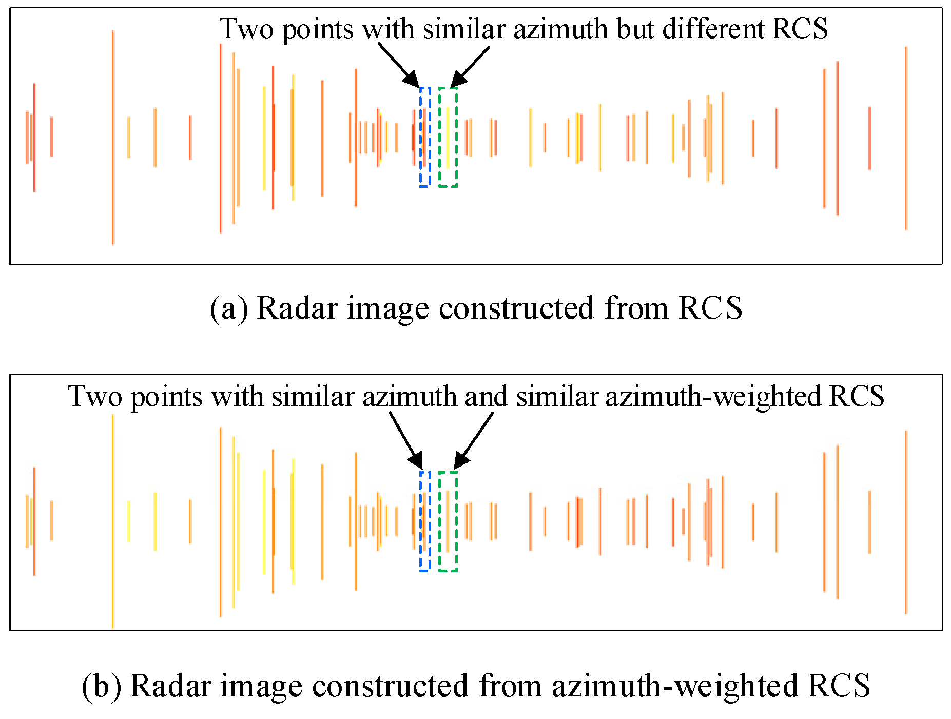
- We introduce a new parameter azimuth-weighted RCS to construct a radar channel, making use of the azimuth and RCS parameters to achieve richer feature representation. Along with velocity, azimuth and azimuth-weighted RCS are chosen to construct additional radar channels and undergo experimental evaluation.
- We present a dual-CBAM-FPN strategy to direct the model’s focus toward pivotal features along the channel and spatial dimensions. CBAM is inserted into both the input and the fusion process of FPN, which significantly enhances the feature representation, particularly with regard to smaller objects.
- Numerous experiments verify the effectiveness of the CRFRD model in improving the detection accuracy of CRF-Net. The weighted mean average precision (wmAP) increases from 43.89% to 45.03%, and more small and occluded objects are detected by CRFRD.
2. Related Work and Background Knowledge
2.1. Related Work
2.2. Radar Data Preprocessing
2.3. CRF-Net
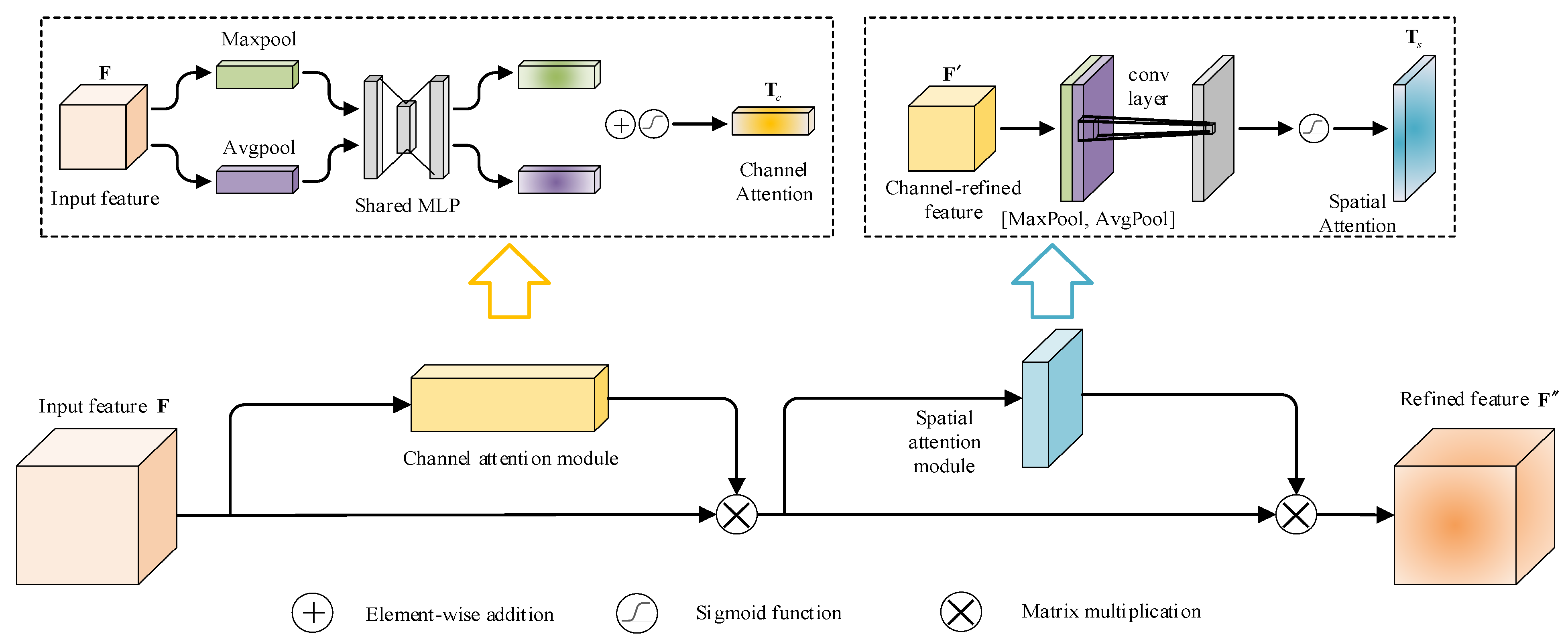
2.4. CBAM
2.4.1. Channel Attention Module
2.4.2. Spatial Attention Module
3. Camera-Radar Fusion with RCE and DCF
3.1. The Overall Structure of CRFRD
3.2. Radar Channel Extension
3.3. Dual-CBAM-FPN
4. Experiment and Analysis of Results
4.1. Dataset and Experimental Settings
4.2. Evaluation Criteria
4.3. Comparative Experiments
4.4. Ablation Study
5. Conclusions
Author Contributions
Funding
Institutional Review Board Statement
Informed Consent Statement
Data Availability Statement
Conflicts of Interest
References
- Bai, J.; Li, S.; Zhang, H.; Huang, L.; Wang, P. Robust Target Detection and Tracking Algorithm Based on Roadside Radar and Camera. Sensors 2021, 21, 1116. [Google Scholar] [CrossRef] [PubMed]
- Liu, P.; Yu, G.; Wang, Z.; Zhou, B.; Chen, P. Object Classification Based on Enhanced Evidence Theory: Radar–Vision Fusion Approach for Roadside Application. IEEE Trans. Instrum. Meas. 2022, 71, 1–12. [Google Scholar] [CrossRef]
- Lin, J.-J.; Guo, J.-I.; Shivanna, V.M.; Chang, S.-Y. Deep Learning Derived Object Detection and Tracking Technology Based on Sensor Fusion of Millimeter-Wave Radar/Video and Its Application on Embedded Systems. Sensors 2023, 23, 2746. [Google Scholar] [CrossRef]
- Ounoughi, C.; Ben Yahia, S. Data Fusion for ITS: A Systematic Literature Review. Inf. Fusion 2023, 89, 267–291. [Google Scholar] [CrossRef]
- Kim, Y.; Kim, S.; Choi, J.W.; Kum, D. CRAFT: Camera-Radar 3D Object Detection with Spatio-Contextual Fusion Transformer. Procee. AAAI Conf. Artif. Intell. 2023, 37, 1160–1168. [Google Scholar] [CrossRef]
- Dudczyk, J.; Czyba, R.; Skrzypczyk, K. Multi-Sensory Data Fusion in Terms of UAV Detection in 3D Space. Sensors 2022, 22, 4323. [Google Scholar] [CrossRef] [PubMed]
- Liu, X.; Li, Z.; Zhou, Y.; Peng, Y.; Luo, J. Camera–Radar Fusion with Modality Interaction and Radar Gaussian Expansion for 3D Object Detection. Cyborg Bionic Syst. 2024, 5, 0079. [Google Scholar] [CrossRef]
- Sun, H.; Feng, H.; Stettinger, G.; Servadei, L.; Wille, R. Multi-Task Cross-Modality Attention-Fusion for 2D Object Detection. In Proceedings of the 2023 IEEE 26th International Conference on Intelligent Transportation Systems (ITSC), Bilbao, Spain, 24–28 September 2023; pp. 3619–3626. [Google Scholar] [CrossRef]
- Zong, M.; Wu, J.; Zhu, Z.; Ni, J. A Method for Target Detection Based on Mmw Radar and Vision Fusion. arXiv 2024, arXiv:2403.16476. [Google Scholar]
- He, S.; Lin, C.; Hu, Z. A Multi-Scale Fusion Obstacle Detection Algorithm for Autonomous Driving Based on Camera and Radar. SAE Intl. J CAV 2023, 6, 333–343. [Google Scholar] [CrossRef]
- Nabati, R.; Qi, H. CenterFusion: Center-Based Radar and Camera Fusion for 3D Object Detection. In Proceedings of the IEEE/CVF Winter Conference on Applications of Computer Vision (WACV), Waikoloa, HI, USA, 3–8 January 2021; pp. 1527–1536. [Google Scholar] [CrossRef]
- Chadwick, S.; Maddern, W.; Newman, P. Distant Vehicle Detection Using Radar and Vision. In Proceedings of the 2019 International Conference on Robotics and Automation (ICRA), Montreal, QC, Canada, 20–24 May 2019; pp. 8311–8317. [Google Scholar] [CrossRef]
- Wang, Z.; Miao, X.; Huang, Z.; Luo, H. Research of Target Detection and Classification Techniques Using Millimeter-Wave Radar and Vision Sensors. Remote Sens. 2021, 13, 1064. [Google Scholar] [CrossRef]
- Ni, J.; Liu, J.; Li, X.; Chen, Z. SFA-Net: Scale and Feature Aggregate Network for Retinal Vessel Segmentation. J. Healthc. Eng. 2022, 2022, e4695136. [Google Scholar] [CrossRef] [PubMed]
- Wang, J.; Kong, L.; Chang, D.; Kong, Z.; Zhao, Y. Interactive Guidance Network for Object Detection Based on Radar-Camera Fusion. Multimedia Tools Appl. 2024, 83, 28057–28075. [Google Scholar] [CrossRef]
- Lo, C.-C.; Vandewalle, P. RCDPT: Radar-Camera Fusion Dense Prediction Transformer. In Proceedings of the IEEE International Conference on Acoustics, Speech, and Signal Processing (ICASSP), Rhodes Island, Greece, 4–10 June 2023; pp. 1–5. [Google Scholar] [CrossRef]
- Nobis, F.; Geisslinger, M.; Weber, M.; Betz, J.; Lienkamp, M. A Deep Learning-Based Radar and Camera Sensor Fusion Architecture for Object Detection. In Proceedings of the 2019 Sensor Data Fusion: Trends, Solutions, Applications (SDF), Bonn, Germany, 15–17 October 2019; pp. 1–7. [Google Scholar] [CrossRef]
- Cui, C.; Ma, Y.; Lu, J.; Wang, Z. REDFormer: Radar Enlightens the Darkness of Camera Perception with Transformers. IEEE Trans. Intell. Veh. 2024, 9, 1358–1368. [Google Scholar] [CrossRef]
- Stacker, L.; Heidenreich, P.; Rambach, J.; Stricker, D. Fusion Point Pruning for Optimized 2D Object Detection with Radar-Camera Fusion. In Proceedings of the 2022 IEEE/CVF Winter Conference on Applications of Computer Vision (WACV), Waikoloa, HI, USA, 5–7 January 2022; pp. 1275–1282. [Google Scholar]
- Xiao, M.; Yang, B.; Wang, S.; Zhang, Z.; Tang, X.; Kang, L. A Feature Fusion Enhanced Multiscale CNN with Attention Mechanism for Spot-Welding Surface Appearance Recognition. Comput. Ind. 2022, 135, 103583. [Google Scholar] [CrossRef]
- Stäcker, L.; Mishra, S.; Heidenreich, P.; Rambach, J.; Stricker, D. RC-BEVFusion: A Plug-In Module for Radar-Camera Bird’s Eye View Feature Fusion. In Proceedings of the DAGM German Conference on Pattern Recognition, Heidelberg, Germany, 19–22 September 2023; pp. 178–194. [Google Scholar] [CrossRef]
- Li, L.; Xie, Y. A Feature Pyramid Fusion Detection Algorithm Based on Radar and Camera Sensor. In Proceedings of the 2020 15th IEEE International Conference on Signal Processing (ICSP), Beijing, China, 6–9 December 2020; pp. 366–370. [Google Scholar] [CrossRef]
- Chang, S.; Zhang, Y.; Zhang, F.; Zhao, X.; Huang, S.; Feng, Z.; Wei, Z. Spatial Attention Fusion for Obstacle Detection Using MmWave Radar and Vision Sensor. Sensors 2020, 20, 956. [Google Scholar] [CrossRef] [PubMed]
- Liu, Y.; Chang, S.; Wei, Z.; Zhang, K.; Feng, Z. Fusing mmWave Radar With Camera for 3-D Detection in Autonomous Driving. IEEE Internet Things J. 2022, 9, 20408–20421. [Google Scholar] [CrossRef]
- Dang, J.; Tang, X.; Li, S. HA-FPN: Hierarchical Attention Feature Pyramid Network for Object Detection. Sensors 2023, 23, 4508. [Google Scholar] [CrossRef]
- Sheng, W.; Yu, X.; Lin, J.; Chen, X. Faster RCNN Target Detection Algorithm Integrating CBAM and FPN. Appl. Sci. 2023, 13, 6913. [Google Scholar] [CrossRef]
- Guo, Q.; Liu, J.; Kaliuzhnyi, M. YOLOX-SAR: High-Precision Object Detection System Based on Visible and Infrared Sensors for SAR Remote Sensing. IEEE Sens. J. 2022, 22, 17243–17253. [Google Scholar] [CrossRef]
- Cerón, J.C.Á.; Ruiz, G.O.; Chang, L.; Ali, S. Real-Time Instance Segmentation of Surgical Instruments Using Attention and Multi-Scale Feature Fusion. Med. Image Anal. 2022, 81, 102569. [Google Scholar] [CrossRef]
- Cui, Z.; Li, Q.; Cao, Z.; Liu, N. Dense Attention Pyramid Networks for Multi-Scale Ship Detection in SAR Images. IEEE Trans. Geosci. Remote Sens. 2019, 57, 8983–8997. [Google Scholar] [CrossRef]
- Han, Y.; Ding, T.; Li, T.; Li, M. An Improved Anchor-Free Object Detection Method. In Proceedings of the 2022 International Conference on Machine Learning and Intelligent Systems Engineering (MLISE), Guangzhou, China, 5–7 August 2022; pp. 6–9. [Google Scholar] [CrossRef]
- Lin, T.L.; Piotr, D.; Ross, G.; He, K.M.; Hariharan, B.; Belongie, S. Feature pyramid networks for object detection. In Proceedings of the IEEE Conference on Computer Vision and Pattern Recognition (CVPR 2017), Honolulu, HI, USA, 22–25 July 2017; pp. 936–944. [Google Scholar]
- Lin, T.Y.; Goyal, P.; Girshick, R.; He, K.M.; Dollár, P. Focal loss for dense object detection. In Proceedings of the IEEE International Conference on Computer Vision (ICCV 2017), Venice, Italy, 22–29 October 2017; pp. 770–778. [Google Scholar]
- Dong, C.; Duoqian, M. Control Distance IoU and Control Distance IoU Loss for Better Bounding Box Regression. Pattern Recognit. 2023, 137, 109256. [Google Scholar] [CrossRef]
- Ganguly, A.; Ruby, A.U.; Chandran J, G.C. Evaluating CNN Architectures Using Attention Mechanisms: Convolutional Block Attention Module, Squeeze, and Excitation for Image Classification on CIFAR10 Dataset. Res. Sq. 2023, 1–13. [Google Scholar] [CrossRef]
- Woo, S.; Park, J.; Lee, J.-Y.; Kweon, I.S. CBAM: Convolutional Block Attention Module. In Proceedings of the European conference on computer vision (ECCV), Munich, Germany, 8–14 September 2018; pp. 3–19. [Google Scholar]
- Zhang, J.; Wu, J.; Wang, H.; Wang, Y.; Li, Y. Cloud Detection Method Using CNN Based on Cascaded Feature Attention and Channel Attention. IEEE Trans. Geosci. Remote Sens. 2022, 60, 1–17. [Google Scholar] [CrossRef]
- Wang, B.; Zhang, S.; Zhang, J.; Cai, Z. Architectural Style Classification Based on CNN and Channel–Spatial Attention. Signal, Image Video Process. 2023, 17, 99–107. [Google Scholar] [CrossRef]
- Caesar, H.; Bankiti, V.; Lang, A.H.; Vora, S.; Liong, V.E.; Xu, Q.; Krishnan, A.; Pan, Y.; Baldan, G.; Beijbom, O. nuScenes: A Multimodal Dataset for Autonomous Driving. In Proceedings of the IEEE/CVF Conference on Computer Vision and Pattern Recognition (CVPR), Seattle, WA, USA, 14–19 June 2020; pp. 11621–11631. [Google Scholar]
- Nabati, R.; Qi, H. Radar-Camera Sensor Fusion for Joint Object Detection and Distance Estimation in Autonomous Vehicles. arXiv 2020, arXiv:2009.08428. [Google Scholar]
- Gu, Y.; Meng, S.; Shi, K. Radar-Enhanced Image Fusion-Based Object Detection for Autonomous Driving. In Proceedings of the 2022 IEEE International Conference on Signal Processing, Communications and Computing (ICSPCC), Xi’an, China, 25–27 October 2022; pp. 1–6. [Google Scholar] [CrossRef]
- Feng, B.; Li, B.; Wang, S.; Ouyang, N.; Dai, W. RSA-Fusion: Radar Spatial Attention Fusion for Object Detection and Classification. Multimed. Tools Appl. 2024, 1–20. [Google Scholar] [CrossRef]
- Sun, H.; Feng, H.; Mauro, G.; Ott, J.; Stettinger, G.; Servadei, L.; Wille, R. Enhanced Radar Perception via Multi-Task Learning: Towards Refined Data for Sensor Fusion Applications. arXiv 2024, arXiv:2404.06165. [Google Scholar]
- Kim, Y.; Shin, J.; Kim, S.; Lee, I.-J.; Choi, J.W.; Kum, D. CRN: Camera Radar Net for Accurate, Robust, Efficient 3D Perception. In Proceedings of the IEEE International Conference on Computer Vision (ICCV 2023), Paris, France, 2–6 October 2023; pp. 17615–17626. [Google Scholar]


| Class | Human | Bicycle | Bus | Car | Motorcycle | Trailer | Truck | wmAP | Parameters | FPS | |
|---|---|---|---|---|---|---|---|---|---|---|---|
| Model | |||||||||||
| RetinaNet [32] | 40.25 | 7.14 | 17.19 | 53.33 | 19.36 | 5.95 | 25.00 | 43.58 | |||
| CRF-Net | 38.41 | 14.99 | 33.67 | 52.96 | 26.60 | 18.37 | 25.85 | 43.89 (43.95 ⊕) | 22.45 M | 4.12 | |
| Nabati and Qi [39] * | 27.59 | 25.00 | 48.30 | 52.31 | 25.97 | 34.45 | 44.49 | ||||
| REF-Net [40] | 44.76 | ||||||||||
| RSA + CA2 [41] | 38.87 | 15.19 | 35.39 | 52.42 | 24.09 | 15.02 | 28.53 | 43.92 | |||
| H. Sun et al. [42] | 44.88 | ||||||||||
| CRFRD | 40.35 | 17.69 | 33.08 | 54.27 | 26.22 | 17.73 | 27.46 | 45.03 | 23.12 M | 3.97 | |
| RCE | DCF | Human | Bicycle | Bus | Car | Motorcycle | Trailer | Truck | wmAP |
|---|---|---|---|---|---|---|---|---|---|
| 38.41 | 14.99 | 33.67 | 52.96 | 26.60 | 18.37 | 25.85 | 43.89 | ||
| √ | 39.66 | 15.23 | 34.76 | 53.79 | 27.69 | 16.29 | 26.43 | 44.74 | |
| √ | 40.26 | 14.78 | 27.25 | 53.14 | 26.35 | 17.37 | 27.48 | 44.41 | |
| √ | √ | 40.35 | 17.69 | 33.08 | 54.27 | 26.22 | 17.73 | 27.46 | 45.03 |
| Human | Bicycle | Bus | Car | Motorcycle | Trailer | Truck | wmAP | ||
|---|---|---|---|---|---|---|---|---|---|
| 39.07 | 13.20 | 28.63 | 53.40 | 22.91 | 18.21 | 26.82 | 44.20 | ||
| √ | 39.64 | 14.44 | 31.41 | 52.93 | 28.50 | 17.05 | 29.18 | 44.49 | |
| √ | 39.66 | 15.23 | 34.76 | 53.79 | 27.69 | 16.29 | 26.43 | 44.74 | |
| √ | √ | 39.90 | 13.28 | 30.20 | 53.68 | 20.40 | 16.86 | 26.34 | 44.52 |
Disclaimer/Publisher’s Note: The statements, opinions and data contained in all publications are solely those of the individual author(s) and contributor(s) and not of MDPI and/or the editor(s). MDPI and/or the editor(s) disclaim responsibility for any injury to people or property resulting from any ideas, methods, instructions or products referred to in the content. |
© 2024 by the authors. Licensee MDPI, Basel, Switzerland. This article is an open access article distributed under the terms and conditions of the Creative Commons Attribution (CC BY) license (https://creativecommons.org/licenses/by/4.0/).
Share and Cite
Sun, X.; Jiang, Y.; Qin, H.; Li, J.; Ji, Y. Camera-Radar Fusion with Radar Channel Extension and Dual-CBAM-FPN for Object Detection. Sensors 2024, 24, 5317. https://doi.org/10.3390/s24165317
Sun X, Jiang Y, Qin H, Li J, Ji Y. Camera-Radar Fusion with Radar Channel Extension and Dual-CBAM-FPN for Object Detection. Sensors. 2024; 24(16):5317. https://doi.org/10.3390/s24165317
Chicago/Turabian StyleSun, Xiyan, Yaoyu Jiang, Hongmei Qin, Jingjing Li, and Yuanfa Ji. 2024. "Camera-Radar Fusion with Radar Channel Extension and Dual-CBAM-FPN for Object Detection" Sensors 24, no. 16: 5317. https://doi.org/10.3390/s24165317
APA StyleSun, X., Jiang, Y., Qin, H., Li, J., & Ji, Y. (2024). Camera-Radar Fusion with Radar Channel Extension and Dual-CBAM-FPN for Object Detection. Sensors, 24(16), 5317. https://doi.org/10.3390/s24165317