
Dense Convolutional Neural Network-Based Deep Learning Pipeline for Pre-Identification of Circular Leaf Spot Disease of Diospyros kaki Leaves Using Optical Coherence Tomography

 ,
,  ,
,  , , , and
Abstract
:1. Introduction
- Developed a DL-based framework using optimized transfer learning models for the automated pre-identification of CLS disease in persimmons, addressing the time-consuming and subjective nature of traditional detection methods.
- Developed a highly curated dataset for CLS classification using manual analysis of OCT amplitude scans (A-scan) and loop-mediated isothermal amplification (LAMP), focusing on pre-identification of CLS.
- Presented the inaugural application of OCT combined with DL for disease detection in plant leaves within agricultural contexts.
- Utilized a novel combination of LAMP with A-scan for detecting CLS disease in persimmon.
2. Related Works
3. Materials and Methodology
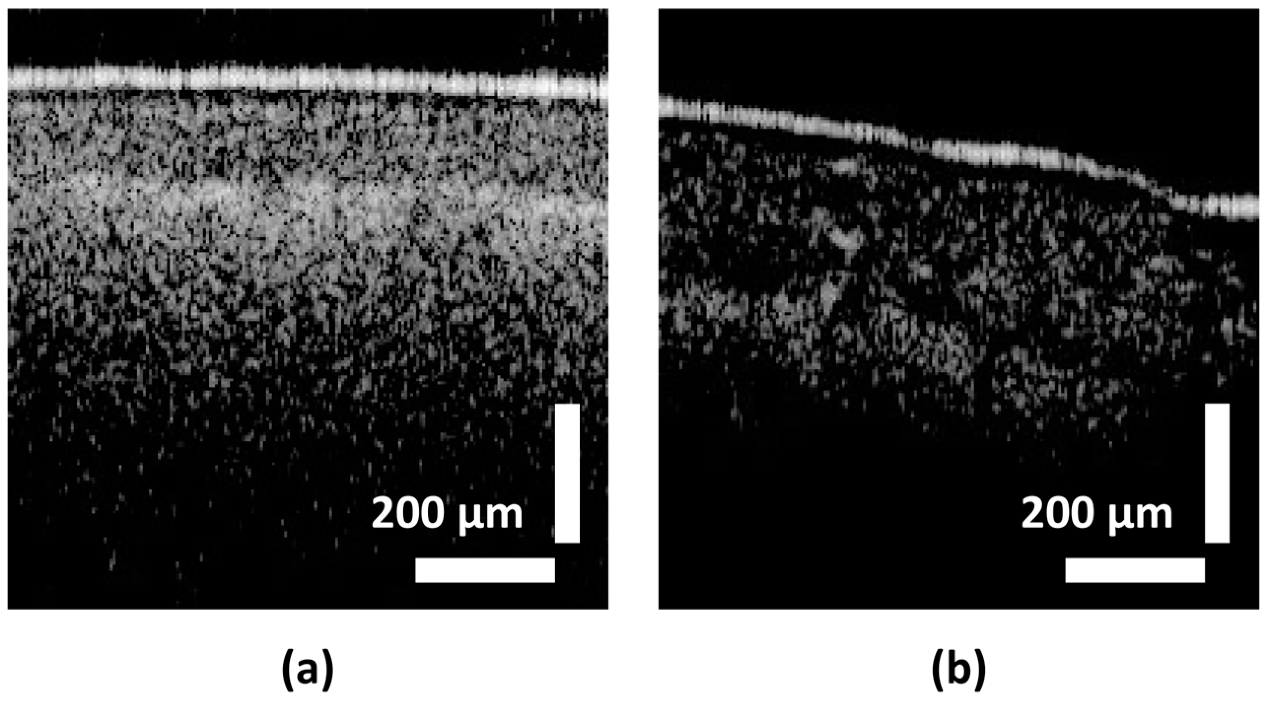
3.1. Experimental Setup and Data Acquisition
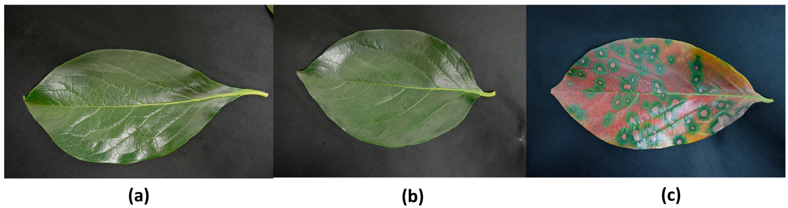
3.1.1. Collection of Plant Materials
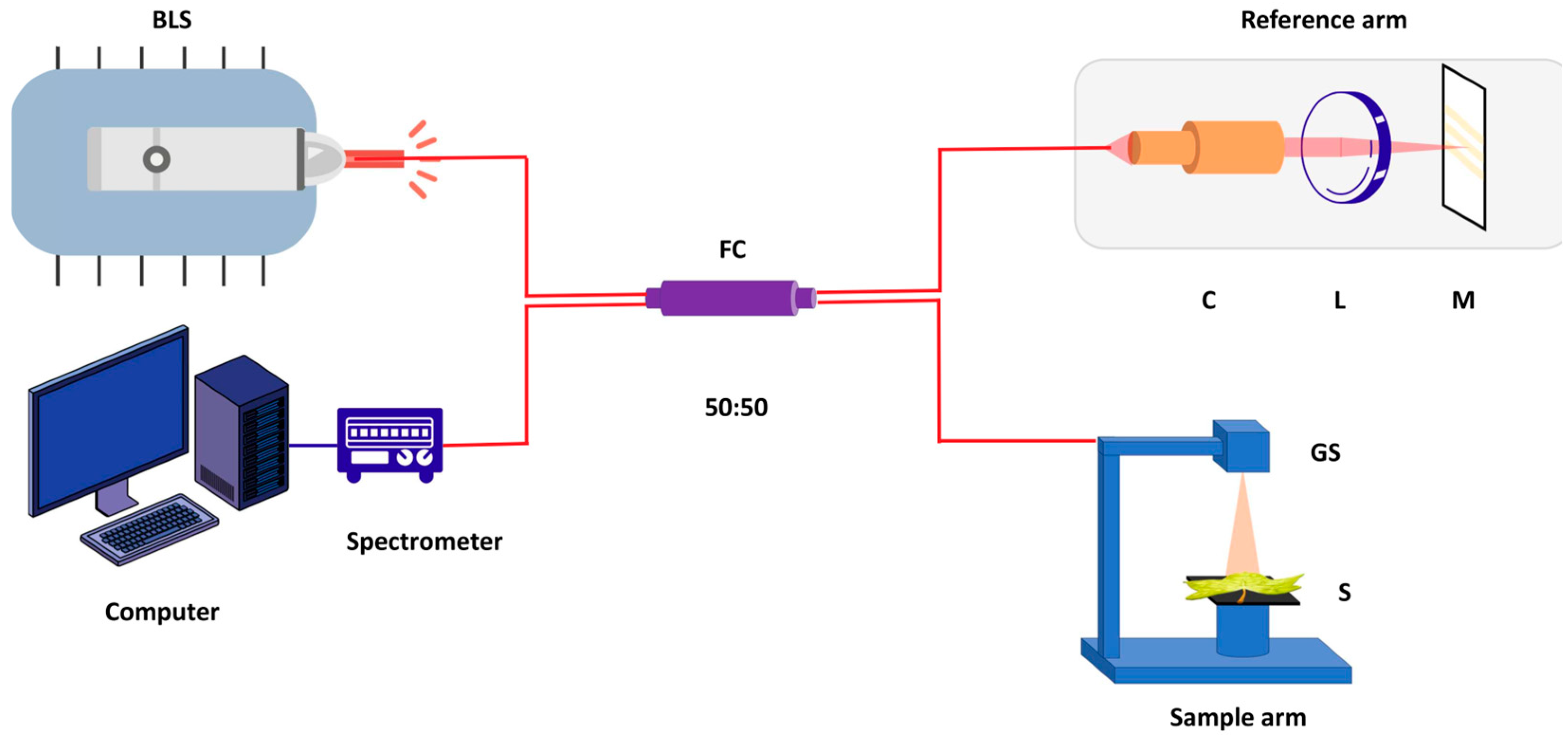
3.1.2. System Configuration
3.1.3. LAMP Technique
3.1.4. Dataset
3.2. Pre-Processing
3.3. Labeling of Datasets
3.4. Deep Learning Models
3.5. Deep Learning Models for Quality Inspection
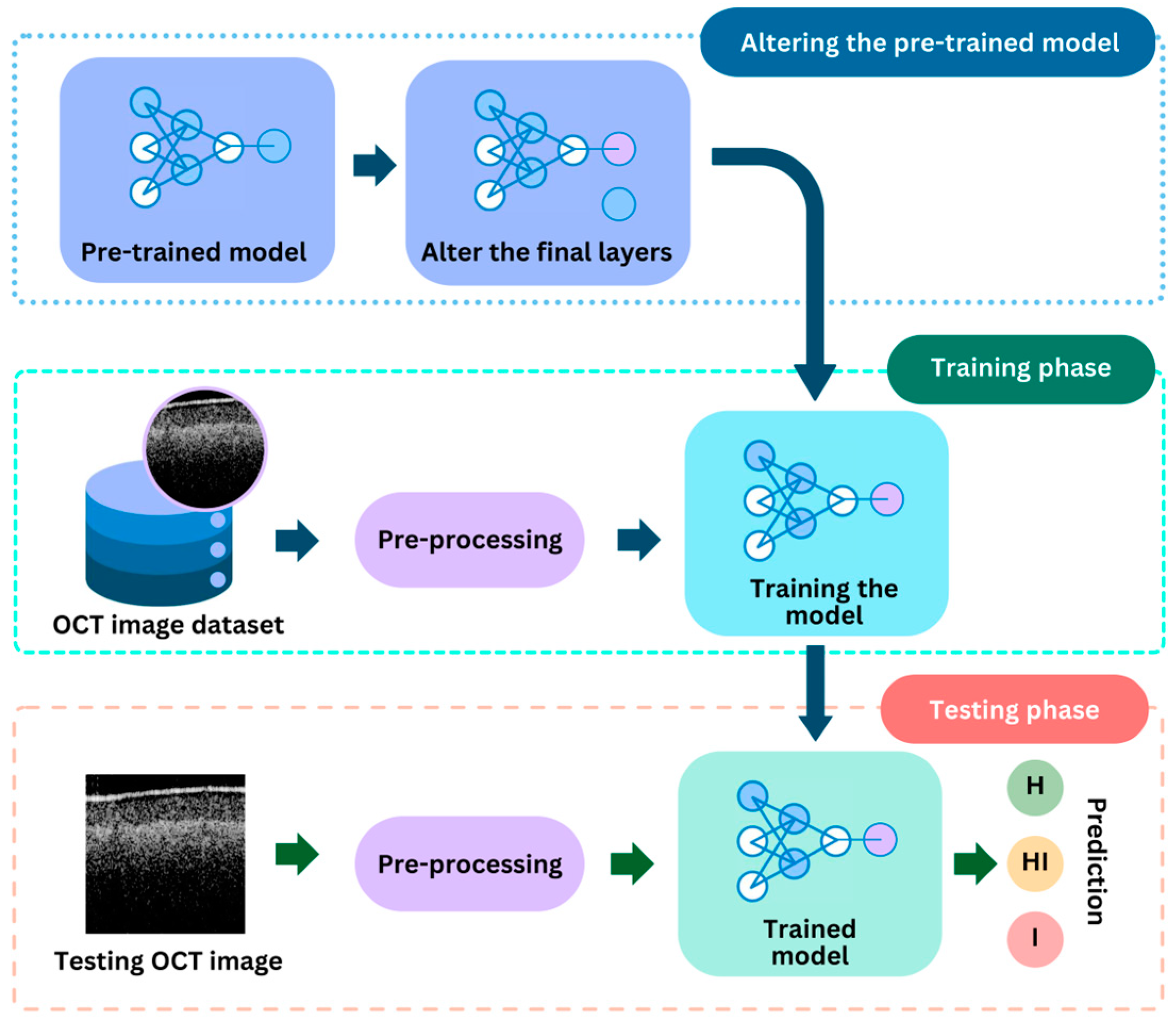
3.6. Deep Learning Model for Identification of Circular Leaf Spot Disease
4. Experimental Results and Analysis
4.1. Quality Inspection Model
4.2. Circular Leaf Spot Disease Detection Model
5. Discussion
6. Conclusions
Supplementary Materials
Author Contributions
Funding
Data Availability Statement
Conflicts of Interest
Abbreviations
| AMD | Age-related macular degeneration |
| ANN | Artificial neural networks |
| AUC | Area under the curve |
| BN | Batch normalization |
| CLS | Circular leaf spot |
| CNN | Convolutional neural network |
| CUDA | Compute unified device architecture |
| DL | Deep learning |
| DME | Diabetic macular edema |
| DNN | Deep neural network |
| FPR | False positive rate |
| GPU | Graphical processing unit |
| GUI | Graphical user interface |
| LAMP | Loop-mediated isothermal amplification |
| ML | Machine learning |
| MRI | Magnetic resonance imaging |
| OA | Overall accuracy |
| OCT | Optical coherence tomography |
| PCR | Polymerase chain reaction |
| ReLU | Rectified linear unit |
| RNN | Recurrent neural network |
| ROC | Receiver operating characteristics |
| SD-OCT | Spectral domain OCT |
| SGD | Stochastic gradient descent |
| TPR | True positive rate |
References
- Hassan, O.; Chang, T. Phylogenetic and Morphological Reassessment of Mycosphaerella nawae, the Causal Agent of Circular Leaf Spot in Persimmon. Plant Dis. 2019, 103, 200–213. [Google Scholar] [CrossRef] [PubMed]
- Choi, O.; Park, J.-J.; Kang, B.; Lee, Y.; Park, J.; Kwon, J.-H.; Kim, J. Evaluation of Ascospore Prediction Model for Circular Leaf Spot Caused by Mycosphaerella nawae of Persimmon. J. Agric. Life Sci. 2018, 52, 13–19. [Google Scholar] [CrossRef]
- Wijesinghe, R.E.; Lee, S.-Y.; Kim, P.; Jung, H.-Y.; Jeon, M.; Kim, J. Optical Inspection and Morphological Analysis of Diospyros Kaki Plant Leaves for the Detection of Circular Leaf Spot Disease. Sensors 2016, 16, 1282. [Google Scholar] [CrossRef] [PubMed]
- Berbegal, M.; Mora-Sala, B.; García-Jiménez, J. A Nested-Polymerase Chain Reaction Protocol for the Detection of Mycosphaerella Nawae in Persimmon. Eur. J. Plant Pathol. 2013, 137, 273–281. [Google Scholar] [CrossRef]
- Singh, V.; Sharma, N.; Singh, S. A Review of Imaging Techniques for Plant Disease Detection. Artif. Intell. Agric. 2020, 4, 229–242. [Google Scholar] [CrossRef]
- Ayache, J.; Beaunier, L.; Boumendil, J.; Ehret, G.; Laub, D. Sample Preparation Handbook for Transmission Electron Microscopy; Springer: New York, NY, USA, 2010; ISBN 978-1-4419-5974-4. [Google Scholar]
- Aniq, H.; Campbell, R. Magnetic Resonance Imaging. In Pain Management; Elsevier: Amsterdam, The Netherlands, 2011; pp. 106–116. ISBN 978-1-4377-0721-2. [Google Scholar]
- Abdhul Rahuman, M.A.; Kahatapitiya, N.S.; Amarakoon, V.N.; Wijenayake, U.; Silva, B.N.; Jeon, M.; Kim, J.; Ravichandran, N.K.; Wijesinghe, R.E. Recent Technological Progress of Fiber-Optical Sensors for Bio-Mechatronics Applications. Technologies 2023, 11, 157. [Google Scholar] [CrossRef]
- Manattayil, J.K.; Ravichandran, N.K.; Wijesinghe, R.E.; Shirazi, M.F.; Lee, S.-Y.; Kim, P.; Jung, H.-Y.; Jeon, M.; Kim, J. Non-Destructive Classification of Diversely Stained Capsicum Annuum Seed Specimens of Different Cultivars Using Near-Infrared Imaging Based Optical Intensity Detection. Sensors 2018, 18, 2500. [Google Scholar] [CrossRef] [PubMed]
- Wijesinghe, R.E.; Lee, S.-Y.; Ravichandran, N.K.; Shirazi, M.F.; Moon, B.; Jung, H.-Y.; Jeon, M.; Kim, J. Bio-Photonic Detection Method for Morphological Analysis of Anthracnose Disease and Physiological Disorders of Diospyros Kaki. Opt. Rev. 2017, 24, 199–205. [Google Scholar] [CrossRef]
- Ravichandran, N.K.; Wijesinghe, R.E.; Shirazi, M.F.; Kim, J.; Jung, H.-Y.; Jeon, M.; Lee, S.-Y. In Vivo Non-Destructive Monitoring of Capsicum Annuum Seed Growth with Diverse NaCl Concentrations Using Optical Detection Technique. Sensors 2017, 17, 2887. [Google Scholar] [CrossRef]
- Yang, D.; Ran, A.R.; Nguyen, T.X.; Lin, T.P.H.; Chen, H.; Lai, T.Y.Y.; Tham, C.C.; Cheung, C.Y. Deep Learning in Optical Coherence Tomography Angiography: Current Progress, Challenges, and Future Directions. Diagnostics 2023, 13, 326. [Google Scholar] [CrossRef]
- Huang, D.; Swanson, E.A.; Lin, C.P.; Schuman, J.S.; Stinson, W.G.; Chang, W.; Hee, M.R.; Flotte, T.; Gregory, K.; Puliafito, C.A.; et al. Optical Coherence Tomography. Science 1991, 254, 1178–1181. [Google Scholar] [CrossRef] [PubMed]
- Bhende, M.; Shetty, S.; Parthasarathy, M.; Ramya, S. Optical Coherence Tomography: A Guide to Interpretation of Common Macular Diseases. Indian J. Ophthalmol. 2018, 66, 20. [Google Scholar] [CrossRef] [PubMed]
- Cho, N.H.; Lee, S.H.; Jung, W.; Jang, J.H.; Kim, J. Optical Coherence Tomography for the Diagnosis and Evaluation of Human Otitis Media. J. Korean Med. Sci. 2015, 30, 328. [Google Scholar] [CrossRef] [PubMed]
- Burwood, G.W.S.; Fridberger, A.; Wang, R.K.; Nuttall, A.L. Revealing the Morphology and Function of the Cochlea and Middle Ear with Optical Coherence Tomography. Quant. Imaging Med. Surg. 2019, 9, 858–881. [Google Scholar] [CrossRef] [PubMed]
- Zeppieri, M.; Marsili, S.; Enaholo, E.S.; Shuaibu, A.O.; Uwagboe, N.; Salati, C.; Spadea, L.; Musa, M. Optical Coherence Tomography (OCT): A Brief Look at the Uses and Technological Evolution of Ophthalmology. Medicina 2023, 59, 2114. [Google Scholar] [CrossRef] [PubMed]
- Hsieh, Y.-S.; Ho, Y.-C.; Lee, S.-Y.; Chuang, C.-C.; Tsai, J.; Lin, K.-F.; Sun, C.-W. Dental Optical Coherence Tomography. Sensors 2013, 13, 8928–8949. [Google Scholar] [CrossRef] [PubMed]
- Sattler, E.; Kästle, R.; Welzel, J. Optical Coherence Tomography in Dermatology. J. Biomed. Opt. 2013, 18, 061224. [Google Scholar] [CrossRef] [PubMed]
- Aumann, S.; Donner, S.; Fischer, J.; Müller, F. Optical Coherence Tomography (OCT): Principle and Technical Realization. In High Resolution Imaging in Microscopy and Ophthalmology: New Frontiers in Biomedical Optics; Bille, J.F., Ed.; Springer International Publishing: Cham, Switzerland, 2019; pp. 59–85. ISBN 978-3-030-16638-0. [Google Scholar]
- Wijesinghe, R.; Lee, S.-Y.; Ravichandran, N.K.; Han, S.; Jeong, H.; Han, Y.; Jung, H.-Y.; Kim, P.; Jeon, M. Optical Coherence Tomography-Integrated, Wearable (Backpack-Type), Compact Diagnostic Imaging Modality for in Situ Leaf Quality Assessment. Appl. Opt. 2017, 56, D108. [Google Scholar] [CrossRef]
- Lee, J.; Lee, S.-Y.; Wijesinghe, R.E.; Ravichandran, N.K.; Han, S.; Kim, P.; Jeon, M.; Jung, H.-Y.; Kim, J. On-Field In Situ Inspection for Marssonina Coronaria Infected Apple Blotch Based on Non-Invasive Bio-Photonic Imaging Module. IEEE Access 2019, 7, 148684–148691. [Google Scholar] [CrossRef]
- Chen, L.; Li, S.; Bai, Q.; Yang, J.; Jiang, S.; Miao, Y. Review of Image Classification Algorithms Based on Convolutional Neural Networks. Remote Sens. 2021, 13, 4712. [Google Scholar] [CrossRef]
- Khurana, D.; Koli, A.; Khatter, K.; Singh, S. Natural Language Processing: State of the Art, Current Trends and Challenges. Multimed. Tools Appl. 2023, 82, 3713–3744. [Google Scholar] [CrossRef]
- Mehrish, A.; Majumder, N.; Bhardwaj, R.; Mihalcea, R.; Poria, S. A Review of Deep Learning Techniques for Speech Processing. arXiv 2023, arXiv:2305.00359. [Google Scholar] [CrossRef]
- Bhattacharya, G. From DNNs to GANs: Review of Efficient Hardware Architectures for Deep Learning. arXiv 2021, arXiv:2107.00092. [Google Scholar] [CrossRef]
- Alzubaidi, L.; Zhang, J.; Humaidi, A.J.; Al-Dujaili, A.; Duan, Y.; Al-Shamma, O.; Santamaría, J.; Fadhel, M.A.; Al-Amidie, M.; Farhan, L. Review of Deep Learning: Concepts, CNN Architectures, Challenges, Applications, Future Directions. J. Big Data 2021, 8, 53. [Google Scholar] [CrossRef]
- Shen, D.; Wu, G.; Suk, H.-I. Deep Learning in Medical Image Analysis. Annu. Rev. Biomed. Eng. 2017, 19, 221–248. [Google Scholar] [CrossRef] [PubMed]
- Tasnim, N.; Hasan, M.; Islam, I. Comparisonal Study of Deep Learning Approaches on Retinal OCT Image. arXiv 2019, arXiv:1912.07783. [Google Scholar]
- Fang, L.; Wang, C.; Li, S.; Rabbani, H.; Chen, X.; Liu, Z. Attention to Lesion: Lesion-Aware Convolutional Neural Network for Retinal Optical Coherence Tomography Image Classification. IEEE Trans. Med. Imaging 2019, 38, 1959–1970. [Google Scholar] [CrossRef]
- Fu, D.J.; Glinton, S.; Lipkova, V.; Faes, L.; Liefers, B.; Zhang, G.; Pontikos, N.; McKeown, A.; Scheibler, L.; Patel, P.J.; et al. Deep-Learning Automated Quantification of Longitudinal OCT Scans Demonstrates Reduced RPE Loss Rate, Preservation of Intact Macular Area and Predictive Value of Isolated Photoreceptor Degeneration in Geographic Atrophy Patients Receiving C3 Inhibition Treatment. Br. J. Ophthalmol. 2024, 108, 536–545. [Google Scholar] [CrossRef] [PubMed]
- Mariottoni, E.B.; Datta, S.; Shigueoka, L.S.; Jammal, A.A.; Tavares, I.M.; Henao, R.; Carin, L.; Medeiros, F.A. Deep Learning–Assisted Detection of Glaucoma Progression in Spectral-Domain OCT. Ophthalmol. Glaucoma 2023, 6, 228–238. [Google Scholar] [CrossRef]
- Marvdashti, T.; Duan, L.; Aasi, S.Z.; Tang, J.Y.; Ellerbee Bowden, A.K. Classification of Basal Cell Carcinoma in Human Skin Using Machine Learning and Quantitative Features Captured by Polarization Sensitive Optical Coherence Tomography. Biomed. Opt. Express 2016, 7, 3721. [Google Scholar] [CrossRef]
- Butola, A.; Prasad, D.K.; Ahmad, A.; Dubey, V.; Qaiser, D.; Srivastava, A.; Senthilkumaran, P.; Ahluwalia, B.S.; Mehta, D.S. Deep Learning Architecture LightOCT for Diagnostic Decision Support Using Optical Coherence Tomography Images of Biological Samples. arXiv 2020, arXiv:1812.02487. [Google Scholar]
- Liu, X.; Ouellette, S.; Jamgochian, M.; Liu, Y.; Rao, B. One-Class Machine Learning Classification of Skin Tissue Based on Manually Scanned Optical Coherence Tomography Imaging. Sci. Rep. 2023, 13, 867. [Google Scholar] [CrossRef] [PubMed]
- Karri, S.P.K.; Chakraborty, D.; Chatterjee, J. Transfer Learning Based Classification of Optical Coherence Tomography Images with Diabetic Macular Edema and Dry Age-Related Macular Degeneration. Biomed. Opt. Express 2017, 8, 579–592. [Google Scholar] [CrossRef] [PubMed]
- Wang, D.; Wang, L. On OCT Image Classification via Deep Learning. IEEE Photonics J. 2019, 11, 3900714. [Google Scholar] [CrossRef]
- Kugelman, J.; Alonso-Caneiro, D.; Read, S.A.; Hamwood, J.; Vincent, S.J.; Chen, F.K.; Collins, M.J. Automatic Choroidal Segmentation in OCT Images Using Supervised Deep Learning Methods. Sci. Rep. 2019, 9, 13298. [Google Scholar] [CrossRef] [PubMed]
- Joshi, D.; Butola, A.; Kanade, S.R.; Prasad, D.K.; Amitha Mithra, S.V.; Singh, N.K.; Bisht, D.S.; Mehta, D.S. Label-Free Non-Invasive Classification of Rice Seeds Using Optical Coherence Tomography Assisted with Deep Neural Network. Opt. Laser Technol. 2021, 137, 106861. [Google Scholar] [CrossRef]
- Manhando, E.; Zhou, Y.; Wang, F. Early Detection of Mold-Contaminated Peanuts Using Machine Learning and Deep Features Based on Optical Coherence Tomography. AgriEngineering 2021, 3, 703–715. [Google Scholar] [CrossRef]
- Benkendorf, D.J.; Hawkins, C.P. Effects of Sample Size and Network Depth on a Deep Learning Approach to Species Distribution Modeling. Ecol. Inform. 2020, 60, 101137. [Google Scholar] [CrossRef]
- Kompanets, I.; Zalyapin, N. Methods and Devices of Speckle-Noise Suppression (Review). Opt. Photonics J. 2020, 10, 219–250. [Google Scholar] [CrossRef]
- Saleah, S.A.; Lee, S.-Y.; Wijesinghe, R.E.; Lee, J.; Seong, D.; Ravichandran, N.K.; Jung, H.-Y.; Jeon, M.; Kim, J. Optical Signal Intensity Incorporated Rice Seed Cultivar Classification Using Optical Coherence Tomography. Comput. Electron. Agric. 2022, 198, 107014. [Google Scholar] [CrossRef]
- Kim, H.E.; Cosa-Linan, A.; Santhanam, N.; Jannesari, M.; Maros, M.E.; Ganslandt, T. Transfer Learning for Medical Image Classification: A Literature Review. BMC Med. Imaging 2022, 22, 69. [Google Scholar] [CrossRef] [PubMed]
- Simonyan, K.; Zisserman, A. Very Deep Convolutional Networks for Large-Scale Image Recognition. arXiv 2014, arXiv:1409.1556. [Google Scholar] [CrossRef]
- Huang, G.; Liu, Z.; Van Der Maaten, L.; Weinberger, K.Q. Densely Connected Convolutional Networks. In Proceedings of the IEEE Conference on Computer Vision and Pattern Recognition, Honolulu, HI, USA, 21–26 July 2017; pp. 4700–4708. [Google Scholar]
- He, K.; Zhang, X.; Ren, S.; Sun, J. Deep Residual Learning for Image Recognition. In Proceedings of the 2016 IEEE Conference on Computer Vision and Pattern Recognition (CVPR), Las Vegas, NV, USA, 27–30 June 2016; pp. 770–778. [Google Scholar]
- Szegedy, C.; Vanhoucke, V.; Ioffe, S.; Shlens, J.; Wojna, Z. Rethinking the Inception Architecture for Computer Vision. In Proceedings of the 2016 IEEE Conference on Computer Vision and Pattern Recognition (CVPR), Las Vegas, NV, USA, 27–30 June 2016; pp. 2818–2826. [Google Scholar]
- Szegedy, C.; Ioffe, S.; Vanhoucke, V.; Alemi, A. Inception-v4, Inception-Resnet and the Impact of Residual Connections on Learning. In Proceedings of the AAAI Conference on Artificial Intelligence, San Francisco, CA, USA, 4–9 February 2017; Volume 31. [Google Scholar]
- Gupta, J.; Pathak, S.; Kumar, G. Deep Learning (CNN) and Transfer Learning: A Review. J. Phys. Conf. Ser. 2022, 2273, 012029. [Google Scholar] [CrossRef]
- Deng, J.; Dong, W.; Socher, R.; Li, L.-J.; Li, K.; Li, F.-F. ImageNet: A Large-Scale Hierarchical Image Database. In Proceedings of the 2009 IEEE Conference on Computer Vision and Pattern Recognition, Miami, FL, USA, 20–25 June 2009; pp. 248–255. [Google Scholar]
- Aoyama, Y.; Maruko, I.; Kawano, T.; Yokoyama, T.; Ogawa, Y.; Maruko, R.; Iida, T. Diagnosis of Central Serous Chorioretinopathy by Deep Learning Analysis of En Face Images of Choroidal Vasculature: A Pilot Study. PLoS ONE 2021, 16, e0244469. [Google Scholar] [CrossRef] [PubMed]
- An, G.; Akiba, M.; Yokota, H.; Motozawa, N.; Takagi, S.; Mandai, M.; Kitahata, S.; Hirami, Y.; Takahashi, M.; Kurimoto, Y. Deep Learning Classification Models Built with Two-Step Transfer Learning for Age Related Macular Degeneration Diagnosis. In Proceedings of the 2019 41st Annual International Conference of the IEEE Engineering in Medicine and Biology Society (EMBC), Berlin, Germany, 23–27 July 2019; pp. 2049–2052. [Google Scholar]
- Lee, C.S.; Baughman, D.M.; Lee, A.Y. Deep Learning Is Effective for the Classification of OCT Images of Normal versus Age-Related Macular Degeneration. Ophthalmol. Retin. 2017, 1, 322–327. [Google Scholar] [CrossRef] [PubMed]
- Sotoudeh-Paima, S.; Jodeiri, A.; Hajizadeh, F.; Soltanian-Zadeh, H. Multi-Scale Convolutional Neural Network for Automated AMD Classification Using Retinal OCT Images. Comput. Biol. Med. 2022, 144, 105368. [Google Scholar] [CrossRef] [PubMed]
- Khan, A.; Pin, K.; Aziz, A.; Han, J.W.; Nam, Y. Optical Coherence Tomography Image Classification Using Hybrid Deep Learning and Ant Colony Optimization. Sensors 2023, 23, 6706. [Google Scholar] [CrossRef]
- Sarah, M.; Mathieu, L.; Philippe, Z.; Guilcher, A.L.; Borderie, L.; Cochener, B.; Quellec, G. Generalizing Deep Learning Models for Medical Image Classification. arXiv 2024, arXiv:2403.12167. [Google Scholar] [CrossRef]


| Class Label | Ranges in µm (∆t) |
|---|---|
| H-healthy | 140+ |
| HI-apparently healthy | 90–130 |
| I-infected | 0–89 |
| A-Scan Label | LAMP Label | Class Label |
|---|---|---|
| H | H | H |
| HI | I | HI |
| I | H | H |
| H | I | HI |
| HI | H | H |
| I | I | I |
| Base Model | Epochs | Loss | Accuracy |
|---|---|---|---|
| VGG16 | 20 | 0.0608 | 0.9899 |
| InceptionResNetV2 | 20 | 0.1088 | 0.9828 |
| InceptionV3 | 50 | 0.1022 | 0.9885 |
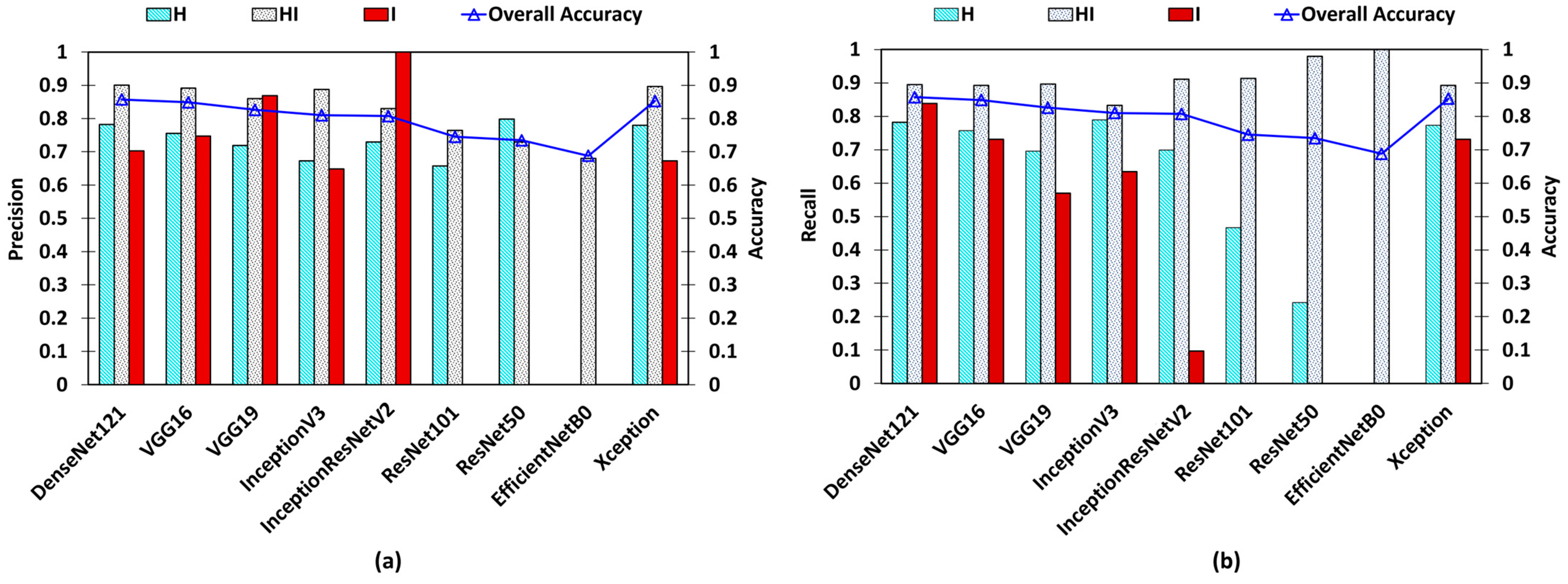
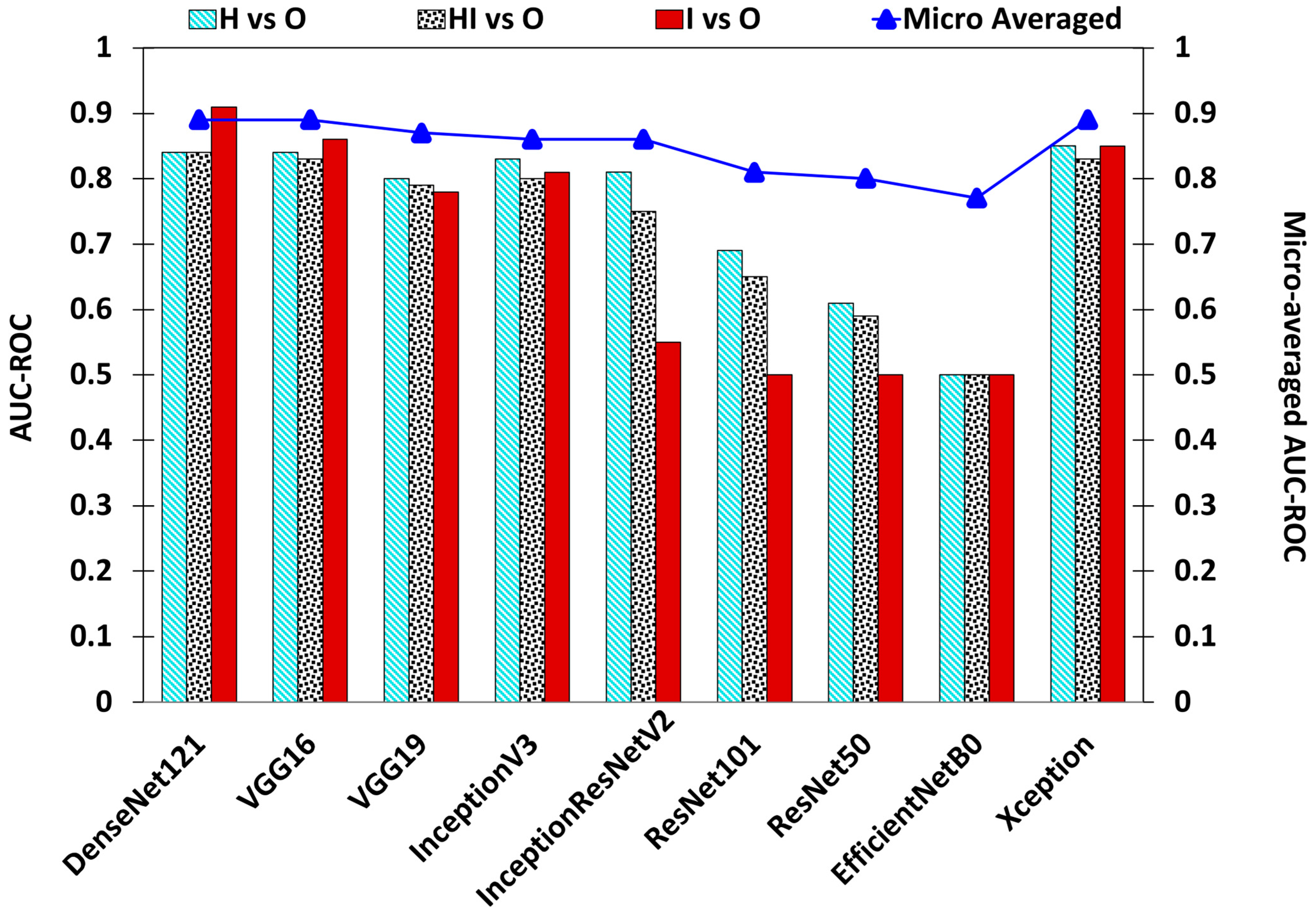
| Base Model | Epochs | Learning Rate | OL | OA | AUC–ROC | Precision | Recall | |||||||
|---|---|---|---|---|---|---|---|---|---|---|---|---|---|---|
| H vs. O | HI vs. O | I vs. O | Micro Averaged | H | HI | I | H | HI | I | |||||
| DenseNet121 | 110 | 0.000125 | 0.3249 | 0.8573 | 0.84 | 0.84 | 0.91 | 0.89 | 0.7823 | 0.9005 | 0.7027 | 0.7573 | 0.8953 | 0.8387 |
| VGG16 | 114 | 0.0001 | 0.369 | 0.8487 | 0.84 | 0.83 | 0.86 | 0.89 | 0.7553 | 0.8915 | 0.7472 | 0.7573 | 0.8924 | 0.7311 |
| VGG19 | 111 | 0.0001 | 0.3861 | 0.826 | 0.8 | 0.79 | 0.78 | 0.87 | 0.719 | 0.8596 | 0.8688 | 0.696 | 0.8963 | 0.5698 |
| InceptionV3 | 82 | 0.0001 | 0.4391 | 0.81 | 0.83 | 0.8 | 0.81 | 0.86 | 0.6727 | 0.8875 | 0.6483 | 0.7893 | 0.833 | 0.6344 |
| InceptionResNetV2 | 109 | 0.0001 | 0.4317 | 0.8073 | 0.81 | 0.75 | 0.55 | 0.86 | 0.7298 | 0.8303 | 1 | 0.6986 | 0.9108 | 0.0967 |
| ResNet101 | 68 | 0.00001 | 0.5815 | 0.7453 | 0.69 | 0.65 | 0.5 | 0.81 | 0.6578 | 0.7641 | 0 | 0.4666 | 0.9137 | 0 |
| ResNet50 | 86 | 0.00001 | 0.5816 | 0.7347 | 0.61 | 0.59 | 0.5 | 0.8 | 0.7982 | 0.7294 | 0 | 0.2426 | 0.9796 | 0 |
| EfficientNetB0 | 122 | 0.0001 | 0.7763 | 0.688 | 0.5 | 0.5 | 0.5 | 0.77 | 0 | 0.688 | 0 | 0 | 1 | 0 |
| Xception | 86 | 0.000125 | 0.3514 | 0.8527 | 0.85 | 0.83 | 0.85 | 0.89 | 0.7795 | 0.8967 | 0.6732 | 0.7733 | 0.8924 | 0.7311 |
Disclaimer/Publisher’s Note: The statements, opinions and data contained in all publications are solely those of the individual author(s) and contributor(s) and not of MDPI and/or the editor(s). MDPI and/or the editor(s) disclaim responsibility for any injury to people or property resulting from any ideas, methods, instructions or products referred to in the content. |
© 2024 by the authors. Licensee MDPI, Basel, Switzerland. This article is an open access article distributed under the terms and conditions of the Creative Commons Attribution (CC BY) license (https://creativecommons.org/licenses/by/4.0/).
Share and Cite
Kalupahana, D.; Kahatapitiya, N.S.; Silva, B.N.; Kim, J.; Jeon, M.; Wijenayake, U.; Wijesinghe, R.E. Dense Convolutional Neural Network-Based Deep Learning Pipeline for Pre-Identification of Circular Leaf Spot Disease of Diospyros kaki Leaves Using Optical Coherence Tomography. Sensors 2024, 24, 5398. https://doi.org/10.3390/s24165398
Kalupahana D, Kahatapitiya NS, Silva BN, Kim J, Jeon M, Wijenayake U, Wijesinghe RE. Dense Convolutional Neural Network-Based Deep Learning Pipeline for Pre-Identification of Circular Leaf Spot Disease of Diospyros kaki Leaves Using Optical Coherence Tomography. Sensors. 2024; 24(16):5398. https://doi.org/10.3390/s24165398
Chicago/Turabian StyleKalupahana, Deshan, Nipun Shantha Kahatapitiya, Bhagya Nathali Silva, Jeehyun Kim, Mansik Jeon, Udaya Wijenayake, and Ruchire Eranga Wijesinghe. 2024. "Dense Convolutional Neural Network-Based Deep Learning Pipeline for Pre-Identification of Circular Leaf Spot Disease of Diospyros kaki Leaves Using Optical Coherence Tomography" Sensors 24, no. 16: 5398. https://doi.org/10.3390/s24165398