

Impact of Land Use and Land Cover (LULC) Changes on Carbon Stocks and Economic Implications in Calabria Using Google Earth Engine (GEE)

Abstract
:1. Background and Related Works
1.1. Background
1.2. Relevant Works
1.3. Overview of the Study
2. Materials and Methods
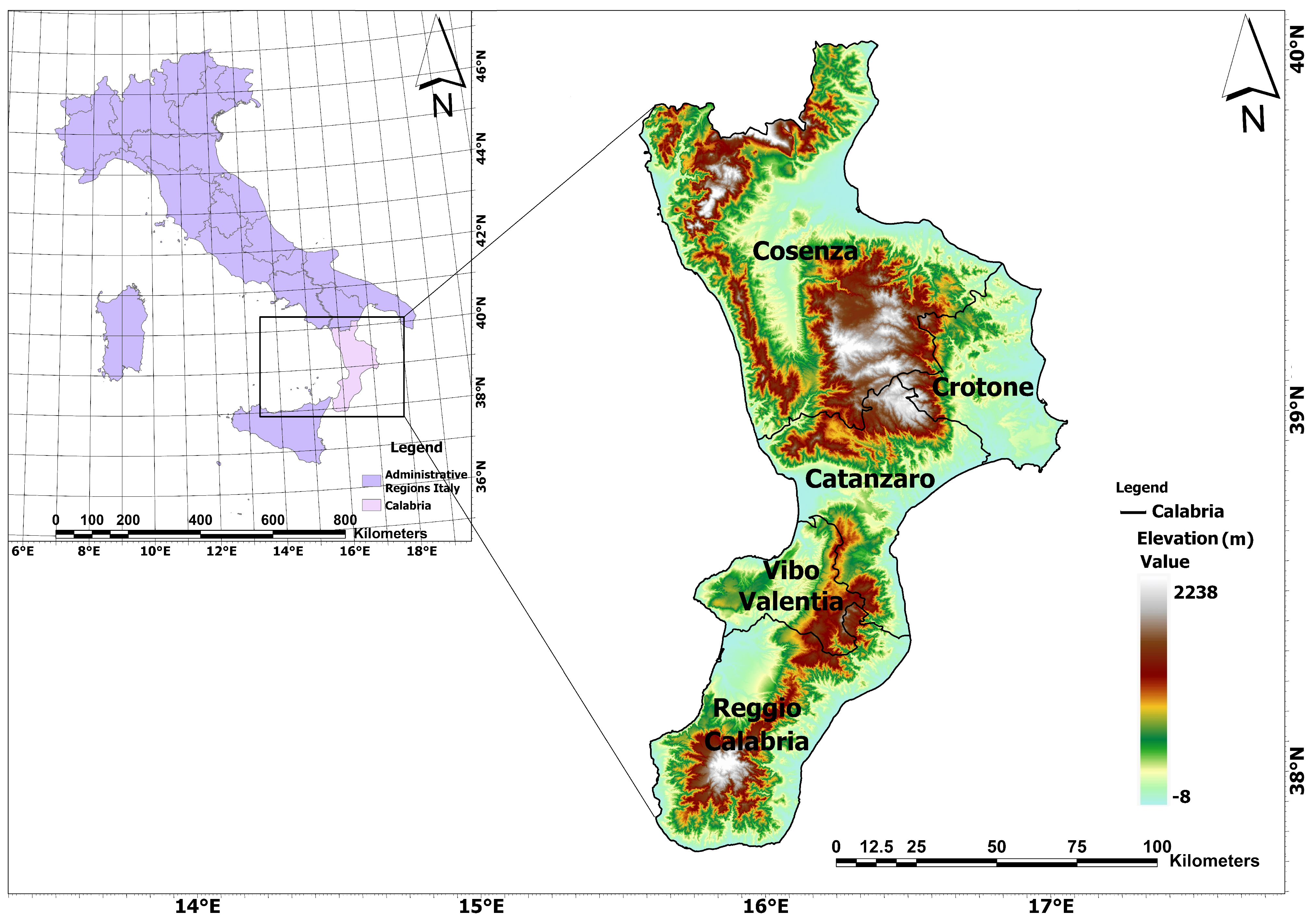
2.1. Study Area
2.2. Data Acquisition
2.3. Data Processing
2.3.1. Preprocessing
2.3.2. LULC Processing
2.3.3. Prediction
- First validation test: The LULC datasets for 2000 and 2006 were used with the average probability matrix to predict the LULC for 2012. The predicted LULC for 2012 was then compared with the actual LULC dataset for 2012.
- Second validation test: Similarly, the LULC datasets for 2006 and 2012 were used to predict the LULC for 2018. The predicted LULC for 2018 was validated by comparing it with the actual LULC dataset for 2018.
2.3.4. Carbon Storage Assessment
Carbon Pools in Forests
Carbon Pools Related to Crops
Carbon Pools Related to Grassland
Carbon Pools Related to Wetland
Carbon Pools Related to Settlements, Water Body, and Other Land
3. Results
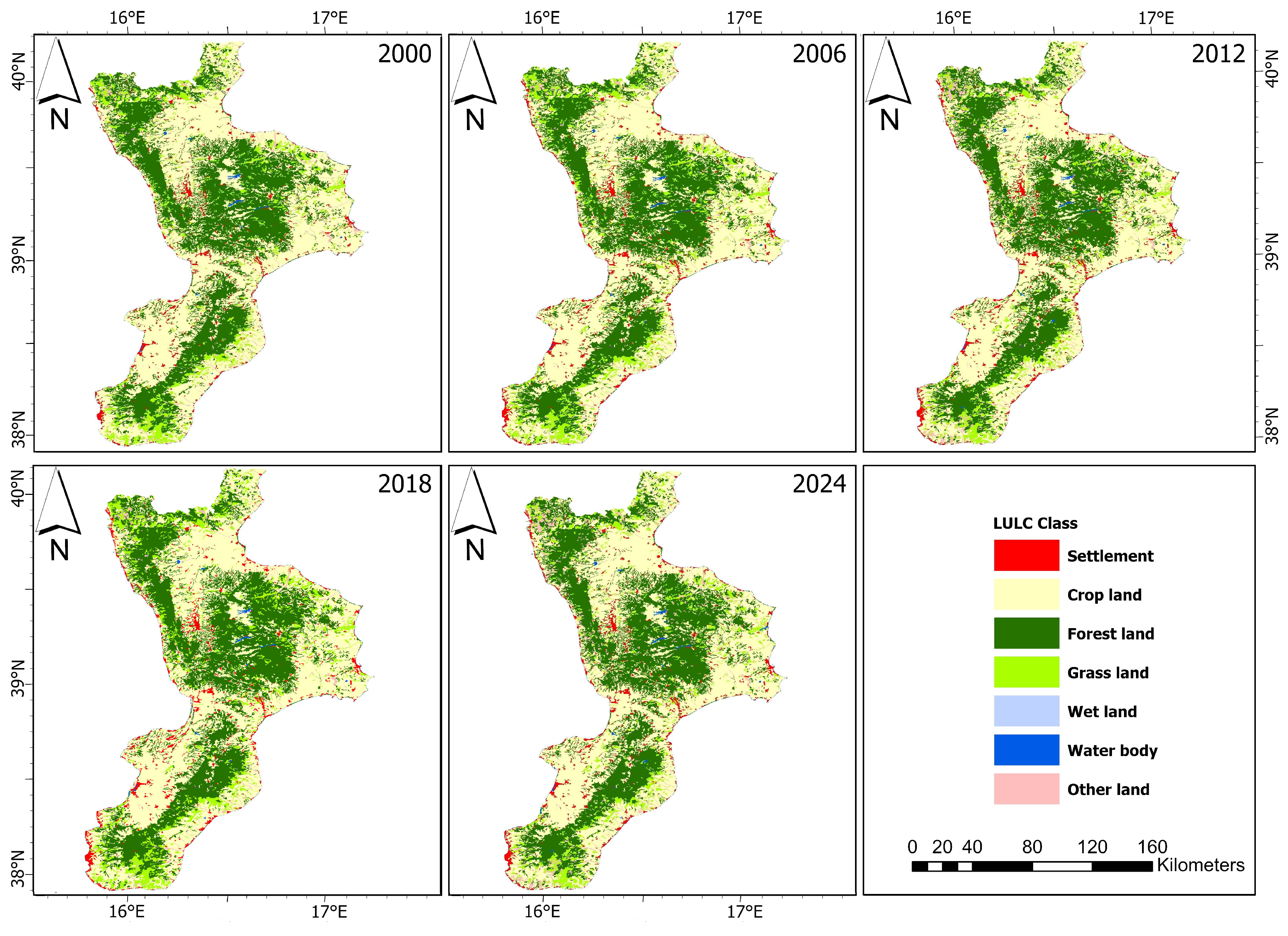
3.1. LULC Scenario
3.2. Validation of CA–Markov Model
3.3. Carbon Scenario
4. Discussion
4.1. Methodological Performance and Limitations
4.2. Changes in LULC
4.3. Changes in Carbon Stocks
4.4. Relationship between Carbon and the Economy
4.5. Interaction between Carbon and Environmental Factors
5. Conclusions
Author Contributions
Funding
Institutional Review Board Statement
Informed Consent Statement
Data Availability Statement
Conflicts of Interest
Abbreviations
| AOI | Area of Interest |
| Average Mortality Rate | |
| Above Ground Biomass | |
| Blow Ground Biomass | |
| Biomass Expansion Factor | |
| CA | Cellular Automata |
| CA–Markov | Cellular Automata-Markov Chain |
| Carbon Above Ground | |
| Carbon Blow Ground | |
| Deadwood Organic Matter Carbon | |
| Carbon Fraction | |
| CLC | Corine Land Cover |
| CO | Carbon dioxide |
| CS | Carbon Sequestration |
| ESs | Ecosystem Services |
| FREL | Forest Reference Emission Level |
| GEE | Google Earth Engine |
| GIS | Geographic Information System |
| Growing Stock | |
| ha | Hectare |
| InVEST | Integrated Valuation of Ecosystem Services and Tradeoffs |
| IPCC | Intergovernmental Panel on Climate Change |
| LULC | Land Use Land Cover |
| LULUCF | Land Use Land Use Change and Forestry |
| Mg | Megagram |
| MgC | Megagram Carbon |
| MRV | Monitoring, Reporting, and Verifying |
| Pg | Petagram |
| REDD | Reducing Emissions from Deforestation and Forest Degradation |
| RS | Remote Sensing |
| SOC | Soil Organic Carbon |
| Tg | Teragram |
| UNFCCC | United Nations Framework Convention on Climate Change |
| Wood Basic Density |
References
- Perrings, C.; Naeem, S.; Ahrestani, F.; Bunker, D.; Burkill, P.; Canziani, G.; Elmqvist, T.; Ferrati, R.; Fuhrman, J.; Jaksic, F.; et al. Ecosystem Services for 2020. Science 2010, 330, 323–324. [Google Scholar] [CrossRef] [PubMed]
- Hasan, S.S.; Zhen, L.; Miah, M.G.; Ahamed, T.; Samie, A. Impact of land use change on Ecosystem Services: A review. Environ. Dev. 2020, 34, 100527. [Google Scholar] [CrossRef]
- Marino, D.; Barone, A.; Marucci, A.; Pili, S.; Palmieri, M. Impact of land use changes on Ecosystem Services supply: A meta analysis of the Italian context. Land 2023, 12, 2173. [Google Scholar] [CrossRef]
- Hassan, R.; Scholes, R.; Ash, N.; Condition, M.; Group, T. Ecosystems and Human Well-Being: Current State and Trends: Findings of the Condition and Trends Working Group; Millennium Ecosystem Assessment Series; Millennium Ecosystem Assessment: Washington, DC, USA, 2005. [Google Scholar]
- Quintas-Soriano, C.; Castro, A.J.; Castro, H.; Garcia Llorente, M. Impacts of land use change on Ecosystem Services and implications for human well-being in Spanish drylands. Land Use Policy 2016, 54, 534–548. [Google Scholar] [CrossRef]
- Selin, N.E. Carbon Sequestration. Encycl. Br. 2024. Available online: https://www.britannica.com/technology/carbon-sequestration (accessed on 6 July 2024).
- Prajapati, S.; Choudhary, S.; Kumar, V.; Dayal, P.; Srivastava, R.; Gairola, A.; Borate, R. Carbon Sequestration: A Key Strategy for Climate Change Mitigation towards a Sustainable Future. Emerg. Trends Clim. Chang. 2023, 2, 1–14. [Google Scholar] [CrossRef]
- Chataut, G.; Bhatta, B.; Joshi, D.; Subedi, K.; Kafle, K. Greenhouse gases emission from agricultural soil: A review. J. Agric. Food Res. 2023, 11, 100533. [Google Scholar] [CrossRef]
- Sharma, S.; Rana, V.S.; Prasad, H.; Lakra, J.; Sharma, U. Appraisal of Carbon Capture, Storage, and Utilization Through Fruit Crops. Front. Environ. Sci. 2021, 9, 700768. [Google Scholar] [CrossRef]
- Scandellari, F.; Caruso, G.; Liguori, G.; Meggio, F.; Palese, A.; Zanotelli, D.; Celano, G.; Gucci, R.; Inglese, P.; Pitacco, A.; et al. A survey of carbon sequestration potential of orchards and vineyards in Italy. Eur. J. Hortic. Sci. 2016, 81, 106–114. [Google Scholar] [CrossRef]
- Zhao, J.; Liu, D.; Zhu, Y.; Peng, H.; Xie, H. A review of forest carbon cycle models on spatiotemporal scales. J. Clean. Prod. 2022, 339, 130692. [Google Scholar] [CrossRef]
- Lama, G.; Rillo Migliorini Giovannini, M.; Errico, A.; Mirzaei, S.; Chirico, G.; Preti, F. The impacts of Nature Based Solutions (NBS) on vegetated flows’ dynamics in urban areas. In Proceedings of the 2021 IEEE International Workshop on Metrology for Agriculture and Forestry (MetroAgriFor), Trento-Bolzano, Italy, 3–5 November 2021; pp. 58–63. [Google Scholar] [CrossRef]
- Grassi, G.; Conchedda, G.; Federici, S.; Abad Viñas, R.; Korosuo, A.; Melo, J.; Rossi, S.; Sandker, M.; Somogyi, Z.; Vizzarri, M.; et al. Carbon fluxes from land 2000–2020: Bringing clarity to countries’ reporting. Earth Syst. Sci. Data 2022, 14, 4643–4666. [Google Scholar] [CrossRef]
- Manchego, C.; Hildebrandt, P.; Cueva, J.; Espinosa, C.; Stimm, B.; Günter, S. Climate change versus deforestation: Implications for tree species distribution in the dry forests of southern Ecuador. PLoS ONE 2017, 12, e0190092, Erratum in PLoS ONE 2018, 13, e0195851. https://doi.org/10.1371/journal.pone.0195851. [Google Scholar] [CrossRef]
- de Groot, R.; Brander, L.; van der Ploeg, S.; Costanza, R.; Bernard, F.; Braat, L.; Christie, M.; Crossman, N.; Ghermandi, A.; Hein, L.; et al. Global estimates of the value of ecosystems and their services in monetary units. Ecosyst. Serv. 2012, 1, 50–61. [Google Scholar] [CrossRef]
- FAO. Global Forest Resources Assessment 2020—Key Findings; FAO: Rome, Italy, 2020. [Google Scholar] [CrossRef]
- REDD+. UNEP—UN Environment Programme. Available online: https://www.unep.org/explore-topics/climate-action/what-we-do/redd (accessed on 4 July 2024).
- Government of Guyana. First REDD+ Technical Annex to the United Nations Framework Convention on Climate Change; Government of Guyana: Georgetown, Guyana, 2024.
- Tomppo, E.; Andersson, K. Technical Review of FAO’s Approach and Methods for National Forest Monitoring and Assessment (NFMA); NFMA Working Paper No. 38; Forestry Department, FAO: Rome, Italy, 2008. [Google Scholar]
- Paneque-Gálvez, J.; McCall, M.; Napoletano, B.; Wich, S.; Koh, L. Small Drones for Community-Based Forest Monitoring: An Assessment of Their Feasibility and Potential in Tropical Areas. Forests 2014, 5, 1481–1507. [Google Scholar] [CrossRef]
- Lama, G.; Crimaldi, M. Assessing the role of Gap Fraction on the Leaf Area Index (LAI) estimations of riparian vegetation based on Fisheye lenses. In Proceedings of the 29th European Biomass Conference and Exhibition, Marseille, France, 26–29 April 2021; pp. 1172–1176. [Google Scholar] [CrossRef]
- Florio, A.; Cutugno, M.; Robustelli, U.; Di Luccio, D.; Pugliano, G.; Benassai, G. Cliff instability evidence from UAV survey observation. In Proceedings of the 2022 IEEE International Workshop on Metrology for the Sea; Learning to Measure Sea Health Parameters (MetroSea), Milazzo, Italy, 3–5 October 2022; pp. 408–413. [Google Scholar] [CrossRef]
- Khachoo, Y.H.; Cutugno, M.; Robustelli, U.; Pugliano, G. Investigating Actual and Future Trends of Thermal Characteristics with Satellite Images and Artificial Neural Networks Approach. In Proceedings of the 2023 IEEE International Workshop on Metrology for the Sea; Learning to Measure Sea Health Parameters (MetroSea), Valletta, Malta, 4–6 October 2023; pp. 67–72. [Google Scholar] [CrossRef]
- Belgiu, M.; Drăguţ, L. Random forest in remote sensing: A review of applications and future directions. ISPRS J. Photogramm. Remote Sens. 2016, 114, 24–31. [Google Scholar] [CrossRef]
- Errico, A.; Lama, G.; Francalanci, S.; Chirico, G.; Solari, L.; Preti, F. Validation of global flow resistance models in two experimental drainage channels covered by Phragmites australis (common reed). In Proceedings of the 38th IAHR World Congress-Water Connecting the World, Panama City, Panama, 1–6 September 2019; pp. 1313–1321. [Google Scholar] [CrossRef]
- Yang, L.; Driscol, J.; Sarigai, S.; Wu, Q.; Chen, H.; Lippitt, C.D. Google Earth Engine and Artificial Intelligence (AI): A Comprehensive Review. Remote Sens. 2022, 14, 3253. [Google Scholar] [CrossRef]
- Prentice, I.; Farquhar, G.; Fasham, M.; Goulden, M.; Heimann, M.; Jaramillo, V.; Kheshgi, H.; Le Quere, C.; Scholes, R.; Wallace, D. The carbon cycle and atmospheric carbon dioxide. In Climate Change 2001: The Scientific Basis. Contribution of Working Group I to the Third Assessment Report of the Intergovernmental Panel on Climate Change (IPCC); Cambridge University Press: Cambridge, UK, 2001; Chapter 3; pp. 183–237. [Google Scholar]
- Shivanna, K. Climate change and its impact on biodiversity and human welfare. Proc. Indian Natl. Sci. Acad. Part A Phys. Sci. 2022, 88, 160–171. [Google Scholar] [CrossRef]
- Lal, R. Carbon Sequestration, Terrestrial. In Reference Module in Earth Systems and Environmental Sciences; Elsevier: Amsterdam, The Netherlands, 2013. [Google Scholar] [CrossRef]
- Guerry, A.; Ruckelshaus, M.; Arkema, K.; Bernhardt, J.; Guannel, G.; Kim, C.K.; Marsik, M.; Papenfus, M.; Toft, J.; Verutes, G.; et al. Modeling benefits from nature: Using Ecosystem Services to inform coastal and marine spatial planning. Int. J. Biodivers. Sci. Ecosyst. Serv. Manag. 2012, 8, 107–121. [Google Scholar] [CrossRef]
- Tallis, H.; Polasky, S. Assessing multiple Ecosystem Services: An integrated tool for the real world. In Natural Capital: Theory and Practice of Mapping Ecosystem Services; Oxford University Press: Oxford, UK, 2011. [Google Scholar] [CrossRef]
- Wang, R.; Zhao, J.; Chen, G.; Lin, Y.; Yang, A.; Cheng, J. Coupling PLUS–InVEST Model for Ecosystem Service Research in Yunnan Province, China. Sustainability 2023, 15, 271. [Google Scholar] [CrossRef]
- Wang, K.; Li, X.; Lyu, X.; Dang, D.; Dou, H.; Li, M.; Liu, S.; Cao, W. Optimizing the Land Use and Land Cover Pattern to Increase Its Contribution to Carbon Neutrality. Remote Sens. 2022, 14, 4751. [Google Scholar] [CrossRef]
- Conradi, T.; Eggli, U.; Kreft, H.; Schweiger, A.H.; Weigelt, P.; Higgins, S.I. Reassessment of the risks of climate change for terrestrial ecosystems. Nat. Ecol. Evol. 2024, 8, 888–900. [Google Scholar] [CrossRef]
- Zhang, M.; Geng, Z.; Yu, Y. Density Functional Theory (DFT) study on the pyrolysis of cellulose: The pyran ring breaking mechanism. Comput. Theor. Chem. 2015, 1067, 13–23. [Google Scholar] [CrossRef]
- Sim, J.; Wright, C.C. The kappa statistic in reliability studies: Use, interpretation, and sample size requirements. Phys. Ther. 2005, 85, 257–268. [Google Scholar] [CrossRef]
- European Commission, E. Geographic Information. Available online: https://circabc.europa.eu/webdav/CircaBC/ESTAT/regportraits/Information/itf6_geo.htm (accessed on 15 July 2024).
- In South Italy Today, M. The Sea Coasts of Southern Italy. Available online: http://www.madeinsouthitalytoday.com/sea-coastes.php (accessed on 15 July 2024).
- Amodio-Morelli, L.; Bonardi, G.; Colonna, V.; Dietrich, D.; Giunta, G.; Ippolito, F.; Liguori, V.; Lorenzoni, S.; Paglionico, A.; Perrone, V.; et al. L’Arco Calabro-Peloritano nell’Orogene Appenninico-Maghrebide. Mem. Della Soc. Geol. Ital. 1976, 17, 1–60. [Google Scholar]
- Gariano, S.L.; Petrucci, O.; Rianna, G.; Santini, M.; Guzzetti, F. Impacts of past and future land changes on landslides in southern Italy. Reg. Environ. Chang. 2018, 18, 437–449. [Google Scholar] [CrossRef]
- LandscapeUNIFI. Calabria. Available online: https://www.landscapeunifi.it/2014/05/27/calabria-en/ (accessed on 11 August 2024).
- European Commission and Directorate-General for Environment and Directorate-General for the Information Society and Media. Corine Land Cover—Technical Guide; Publications Office: Luxembourg, 1994. [Google Scholar]
- Büttner, G.; Kosztra, B. CLC2018 Technical Guidelines; Contribution by Soukup, Tomas, Sousa, Ana, and Langanke, Tobias. Based on CLC2006 Technical guidelines (EEA Technical report No 17/2007) and CLC2012 Addendum to the CLC2006 Technical Guidelines (ETC/SIA Report); Technical Report; European Environment Agency: Copenhagen, Denmark, 2017. [Google Scholar]
- Eggleston, H.; Buendia, L.; Miwa, K.; Ngara, T.; Tanabe, K. 2006 IPCC Guidelines for National Greenhouse Gas Inventories; Technical Report; IPCC: Geneva, Switzerland, 2006. [Google Scholar]
- Zheng, H.; Zheng, H. Assessment and prediction of carbon storage based on land use/land cover dynamics in the coastal area of Shandong Province. Ecol. Indic. 2023, 153, 110474. [Google Scholar] [CrossRef]
- Khachoo, Y.H.; Cutugno, M.; Robustelli, U.; Pugliano, G. Machine Learning for Quantification of Land Transitions in Italy Between 2000 and 2018 and Prediction for 2050. In Proceedings of the 2022 IEEE International Workshop on Metrology for the Sea; Learning to Measure Sea Health Parameters (MetroSea), Milazzo, Italy, 3–5 October 2022; pp. 225–230. [Google Scholar] [CrossRef]
- Weng, Q. Land use change analysis in the Zhujiang Delta of China using satellite remote sensing, GIS and stochastic modelling. Environ. Manag. 2002, 64, 273–284. [Google Scholar] [CrossRef] [PubMed]
- Singh, S.K.; Mustak, S.; Srivastava, P.K.; Szabó, S.; Islam, T. Predicting spatial and decadal LULC changes through cellular automata Markov chain models using earth observation datasets and geo-information. Environ. Process. 2015, 2, 61–78. [Google Scholar] [CrossRef]
- Chen, L.; Nuo, W. Dynamic simulation of land use changes in Port city: A case study of Dalian, China. Procedia-Soc. Behav. Sci. 2013, 96, 981–992. [Google Scholar] [CrossRef]
- Katana, S.J.S.; Ucakuwun, E.K.; Munyao, T.M. Detection and prediction of land cover changes in upper Athi River catchment, Kenya: A strategy towards monitoring environmental changes. Greener J. Environ. Manag. Public Saf. 2013, 2, 146–157. [Google Scholar] [CrossRef]
- Berger, T. Agent-based spatial models applied to agriculture: A simulation tool for technology diffusion, resource use changes and policy analysis. Agric. Econ. 2001, 25, 245–260. [Google Scholar] [CrossRef]
- Aitkenhead, M.J.; Aalders, I.H. Automating land cover mapping of Scotland using expert system and knowledge integration methods. Remote Sens. Environ. 2011, 115, 1285–1295. [Google Scholar] [CrossRef]
- Pontius, G.; Malanson, J. Comparison of the structure and accuracy of two land change models. Int. J. Geogr. Inf. Sci. 2005, 19, 243–265. [Google Scholar] [CrossRef]
- Fan, F.; Wang, Y.; Wang, Z. Temporal and spatial change detecting (1998–2003) and predicting of land use and land cover in Core corridor of Pearl River Delta (China) by using TM and ETM + images. Environ. Monit. Assess. 2008, 137, 127–147. [Google Scholar] [CrossRef] [PubMed]
- Parsa, V.; Yavari, A.; Nejadi, A. Spatio-temporal analysis of land use/land cover pattern changes in Arasbaran Biosphere Reserve: Iran. Model. Earth Syst. Environ. 2016, 4, 1–13. [Google Scholar] [CrossRef]
- Moser, G.; Serpico, S.; Benediktsson, J. Land-cover mapping by Markov modeling of spatial-contextual information in very-high-resolution remote sensing images. Proc. IEEE 2013, 101, 631–651. [Google Scholar] [CrossRef]
- Khachoo, Y.H.; Cutugno, M.; Robustelli, U.; Pugliano, G. Unveiling the dynamics of thermal characteristics related to lulc changes via ann. Sensors 2023, 23, 7013. [Google Scholar] [CrossRef]
- Natural Capital Project. InVEST 3.14.2; Stanford University, University of Minnesota, Chinese Academy of Sciences, The Nature Conservancy, World Wildlife Fund, Stockholm Resilience Centre and the Royal Swedish Academy of Sciences: Stockhom, Sweden, 2024. [Google Scholar]
- Penman, J.; Gytarsky, M.; Hiraishi, T.; Krug, T.; Kruger, D.; Pipatti, R.; Buendia, L.; Miwa, K.; Ngara, T.; Tanabe, K.; et al. Good Practice Guidance for Land Use, Land-Use Change and Forestry; Technical Report; IPCC: Hayama, Japan, 2003. [Google Scholar]
- Core Writing Team; Pachauri, R.K.; Meyer, L.A. (Eds.) Climate Change 2014: Synthesis Report. Contribution of Working Groups I, II and III to the Fifth Assessment Report of the Intergovernmental Panel on Climate Change; Technical Report; IPCC: Geneva, Switzerland, 2014. [Google Scholar]
- Ma, T.; Li, X.; Bai, J.; Ding, S.; Zhou, F.; Cui, B. Four decades’ dynamics of coastal blue carbon storage driven by land use/land cover transformation under natural and anthropogenic processes in the Yellow River Delta, China. Sci. Total Environ. 2019, 655, 741–750. [Google Scholar] [CrossRef]
- Gasparini, P.; Di Cosmo, L.; Floris, A.; De Laurentis, D. Italian National Forest Inventory—Methods and Results of the Third Survey: Inventario Nazionale delle Foreste e dei Serbatoi Forestali di Carbonio—Metodi e Risultati della Terza Indagine; Springer: Cham, Switzerland, 2022. [Google Scholar] [CrossRef]
- Romano, D.; Arcarese, C.; Bernetti, A.; Caputo, A.; Cordella, M.; Lauretis, R.D.; Cristofaro, E.D.; Gagna, A.; Gonella, B.; Moricci, F.; et al. Italian Greenhouse Gas Inventory 1990–2021: National Inventory Report 2023; ISPRA—Institute for Environmental Protection and Research: Roma, Italy, 2023; ISBN 978-88-448-1155-6. [Google Scholar]
- Aalde, H.; Gonzalez, P.; Gytarsky, M.; Krug, T.; Kurz, W.; Ogle, S.; Raison, J.; Schoene, D.; Ravindranath, N.; Elhassan, N. IPCC guidelines for national greenhouse gas inventories. For. Land 2006, 157–169. [Google Scholar]
- Federici, S.; Vitullo, M.; Tulipano, S.; De Lauretis, R.; Seufert, G. An approach to estimate carbon stocks change in forest carbon pools under the UNFCCC: The Italian case. IForest-Biogeosci. For. 2008, 1, 86. [Google Scholar] [CrossRef]
- Zhang, Z.; Jiang, W.; Peng, K.; Wu, Z.; Ling, Z.; Li, Z. Assessment of the impact of wetland changes on carbon storage in coastal urban agglomerations from 1990 to 2035 in support of SDG15.1. Sci. Total Environ. 2023, 877, 162824. [Google Scholar] [CrossRef]
- Babbar, D.; Areendran, G.; Sahana, M.; Sarma, K.; Raj, K.; Sivadas, A. Assessment and prediction of carbon sequestration using Markov chain and InVEST model in Sariska Tiger Reserve, India. J. Clean. Prod. 2021, 278, 123333. [Google Scholar] [CrossRef]
- Tallis, H.T.; Ricketts, T.; Guerry, A.D.; Wood, S.A.; Sharp, R.; Nelson, E.; Pennington, D. Capital Project: Stanford. InVEST 2.5.6 User’s Guide; Natural Capital Project: Stanford, CA, USA, 2013. [Google Scholar]
- Occasional Paper Series Climate Change and Monetary Policy in the Euro Area Work Stream on Climate Change. Available online: https://op.europa.eu/en/publication-detail/-/publication/60bf2a67-2194-11ec-bd8e-01aa75ed71a1/language-en (accessed on 26 July 2024). [CrossRef]
- Thomson, A.M.; César Izaurralde, R.; Smith, S.J.; Clarke, L.E. Integrated estimates of global terrestrial carbon sequestration. Glob. Environ. Chang. 2008, 18, 192–203. [Google Scholar] [CrossRef]
- Engel, S.; Pagiola, S.; Wunder, S. Designing payments for environmental services in theory and practice: An overview of the issues. Ecol. Econ. 2008, 65, 663–674. [Google Scholar] [CrossRef]
- Stern, N. The Economics of Climate Change: The Stern Review; Cambridge University Press: Cambridge, UK, 2007. [Google Scholar] [CrossRef]
- Nishina, K.; Ito, A.; Beerling, D.; Cadule, P.; Ciais, P.; Clark, D.; Falloon, P.; Friend, A.; Kahana, R.; Kato, E.; et al. Quantifying uncertainties in soil carbon responses to changes in global mean temperature and precipitation. Earth Syst. Dyn. 2014, 5, 197–209. [Google Scholar] [CrossRef]
- Bronick, C.; Lal, R. Soil structure and management: A review. Geoderma 2005, 124, 3–22. [Google Scholar] [CrossRef]
- Conant, R.; Ryan, M.; Ågren, G.; Birgé, H.; Davidson, E.; Eliasson, P.; Evans, S.; Frey, S.; Giardina, C.; Hopkins, F.; et al. Temperature and soil organic matter decomposition rates – synthesis of current knowledge and a way forward. Glob. Chang. Biol. 2011, 17, 3392–3404. [Google Scholar] [CrossRef]
- Zhang, R.; Zhao, X.; Zuo, X.; Qu, H.; Degen, A.A.; Luo, Y.; Ma, X.; Chen, M.; Liu, L.; Chen, J. Impacts of Precipitation on Ecosystem Carbon Fluxes in Desert-Grasslands in Inner Mongolia, China. J. Geophys. Res. Atmos. 2019, 124, 1266–1276. [Google Scholar] [CrossRef]
- Xu, Z.; Tsang, D.C. Mineral-mediated stability of organic carbon in soil and relevant interaction mechanisms. Eco-Environ. Health 2024, 3, 59–76. [Google Scholar] [CrossRef]
- Meier, I.C.; Leuschner, C. Variation of soil and biomass carbon pools in beech forests across a precipitation gradient. Glob. Chang. Biol. 2010, 16, 1035–1045. [Google Scholar] [CrossRef]
- Curtin, D.; Beare, M.H.; Hernandez-Ramirez, G. Temperature and Moisture Effects on Microbial Biomass and Soil Organic Matter Mineralization. Soil Sci. Soc. Am. J. 2012, 76, 2055–2067. [Google Scholar] [CrossRef]
- Franzluebbers, A.; Haney, R.; Honeycutt, C.; Arshad, M.; Schomberg, H.; Hons, F. Climatic influences on active fractions of soil organic matter. Soil Biol. Biochem. 2001, 33, 1103–1111. [Google Scholar] [CrossRef]
- Verra. Verified Carbon Standard (VCS). Available online: https://verra.org/programs/verified-carbon-standard/ (accessed on 26 July 2024).


| LULC Class | Description | Corine Landcover Classes Combined |
|---|---|---|
| Settlement | Areas dominated by infrastructure | (1) Continuous urban fabric; (2) Discontinuous urban fabric; (3) Industrial or commercial units; (4) Road and rail networks and land; (5) Port areas; (6) Airports; (7) Mineral extractions sites; (8) Dump sites; (9) Construction sites; (10) Green urban areas; (11) Sport and leisure facilities. |
| Crop land | Areas where farming is performed | (1) Non-irrigated arable land; (2) Permanently irrigated land; (3) Rice fields; (4) Vineyards; (5) Fruit trees and berry plantations; (6) Olive grooves; (7) Annual crops associated with permanent crops; (8) Complex cultivation patterns; (9) Land principally occupied by agriculture, with significant area of natural vegetation. |
| Forest land | Areas with high-density of trees | (1) Agro-forestry areas; (2) Broad-leaved forest; (3) Coniferous forest; (4) Mixed forest. |
| Grassland | Green areas with no or sparse tree cover | (1) Natural grasslands; (2) Moors and heathland; (3) Sclerophyllous vegetation; (4) Transitional woodland-shrub; (5) Pastures; (6) Sparse vegetative areas. |
| Wetland | Damped or wet areas | (1) Inland marshes; (2) Peat bogs; (3) Salt marshes; (4) Salines; (5) Intertidal flats. |
| Water body | Areas partially or totally covered by water | (1) Water courses; (2) water bodies; (3) Coastal lagoons; (4) Estuaries; (5) Sea and ocean. |
| Other land | Areas with no vegetation | (1) Beaches, dunes, sands; (2) Bare soil and rocks; (3) Burnt areas; (4) Glaciers and perpetual snow. |
| Settlement | Crop Land | Forest Land | Grassland | Wet Land | Water Body | Other Land | |
|---|---|---|---|---|---|---|---|
| Settlement | 0.9862 | 0.0081 | 0.0019 | 0.0028 | 0.0000 | 0.0005 | 0.0004 |
| Crop land | 0.0058 | 0.9860 | 0.0019 | 0.0058 | 0.0000 | 0.0001 | 0.0003 |
| Forest land | 0.0001 | 0.0035 | 0.9872 | 0.0083 | 0.0000 | 0.0001 | 0.0007 |
| Grassland | 0.0004 | 0.0134 | 0.0253 | 0.8977 | 0.0000 | 0.0024 | 0.0607 |
| Wet land | 0.0000 | 0.0000 | 0.0000 | 0.1070 | 0.7920 | 0.1009 | 0.0000 |
| Water body | 0.0009 | 0.0008 | 0.0000 | 0.0000 | 0.0000 | 0.9963 | 0.0020 |
| Other land | 0.0007 | 0.0086 | 0.0083 | 0.0688 | 0.0000 | 0.0006 | 0.9131 |
| Biomass Expansion Factor | Wood Basic Density | Carbon Fraction | Root to Shoot Ratio | Average Mortality Rate | |
|---|---|---|---|---|---|
| Forest Tree Type | (R) | ||||
| European beech | 1.36 | 0.61 | 0.47 | 0.20 | 0.0177 |
| Chestnut | 1.33 | 0.49 | 0.47 | 0.28 | 0.0177 |
| Turkey oak | 1.45 | 0.69 | 0.47 | 0.24 | 0.0177 |
| Larches | 1.22 | 0.56 | 0.47 | 0.29 | 0.0177 |
| Mean value | 1.34 | 0.58 | 0.47 | 0.25 | 0.0177 |
| Crop Type | Maturity Cycle (Years) | Carbon above Ground | Carbon below Ground |
|---|---|---|---|
| Olive | 50 | 9.13 | 2.60 |
| Vineyards (wine grapes) | 20 | 5.6 | 4.46 |
| Vineyards (other) | 30 | 5.62 | 4.48 |
| Orchards | 25 | 8.91 | 5.75 |
| Other fruits | 20 | 8.90 | 5.73 |
| Mean value | - | 7.63 | 4.60 |
| Wetland Type | Carbon above Ground | Carbon below Ground | Soil Carbon | Dead Organic Matter Carbon |
|---|---|---|---|---|
| () | () | () | () | |
| Swamp | 18.00 | 18.50 | 161.50 | 10.00 |
| Lake related wetland | 6.00 | 19.50 | 11.50 | 0 |
| River related wetland | 6.00 | 32.00 | 71.50 | 0 |
| Beach related wetland | 39.00 | 19.50 | 62.00 | 10.00 |
| Mangrove wetland | 48.50 | 106.00 | 206.00 | 3.00 |
| Pond related wetland | 18.00 | 6.50 | 17.00 | 0 |
| Mean value | 22.58 | 33.66 | 88.25 | 3.83 |
| Carbon above Ground | Carbon below Ground | Soil Carbon | Dead Organic Matter Carbon | |
|---|---|---|---|---|
| LULC Class | () | () | () | () |
| Settlement | 2 | 1 | 5 | 0 |
| Crop land | 8 | 5 | 46 | 1 |
| Forest land | 93 | 17 | 83 | 9 |
| Grassland | 1 | 5 | 66 | 0 |
| Wet land | 23 | 34 | 88 | 4 |
| Water body | 2 | 1 | 10 | 0 |
| Other land | 2 | 0 | 16 | 0 |
| LULC Classes | LULC 2000 | LULC 2006 | LULC 2012 | LULC 2018 | LULC 2024 |
|---|---|---|---|---|---|
| [km] (%) | [km] (%) | [km] (%) | [km] (%) | [km] (%) | |
| Settlement | 446.66 (2.95%) | 547.42 (3.62%) | 560.15 (3.70%) | 560.05 (3.70%) | 580.95 (3.84%) |
| Crop land | 7319.45 (48.41%) | 7180.98 (47.50%) | 7151.97 (47.30%) | 7151.02 (47.30%) | 7121.24 (47.10%) |
| Forest land | 5536.18 (36.62%) | 5482.54 (36.26%) | 5469.46 (36.18%) | 5488.18 (36.30%) | 5469.74 (36.18%) |
| Grassland | 1482.16 (9.80%) | 1615.02 (10.68%) | 1353.51 (8.95%) | 1329.28 (8.79%) | 1306.74 (8.64%) |
| Wet land | 1.25 (0.01%) | 0.47 (0.00%) | 0.47 (0.00%) | 0.47 (0.00%) | 0.47 (0.00%) |
| Water body | 70.38 (0.47%) | 73.52 (0.49%) | 76.92 (0.51%) | 83.84 (0.55%) | 86.88 (0.57%) |
| Other land | 262.77 (1.74%) | 218.89 (1.45%) | 506.37 (3.35%) | 505.99 (3.35%) | 553.56 (3.66%) |
| Type | Year | ||||
|---|---|---|---|---|---|
| LULC | 2012 | 0.9656 | 0.9773 | 0.9755 | 0.9755 |
| LULC | 2018 | 0.9814 | 0.9877 | 0.9854 | 0.9854 |
| Agreement/Disagreement | LULC 2012 | LULC 2018 |
|---|---|---|
| Agreement due to chance | 0.1250 | 0.1250 |
| Agreement due to quantity | 0.2976 | 0.2973 |
| Agreement at stratum level | 0.0000 | 0.0000 |
| Agreement at gridcell level | 0.5575 | 0.5669 |
| Disagreement at gridcell level | 0.0140 | 0.0084 |
| Disagreement at stratum level | 0.0000 | 0.0000 |
| Disagreement due to quantity | 0.0059 | 0.0023 |
| Year | Stored Carbon | Economic Value of Stored Carbon | Variation | Equivalent Units of CO | Economic Value of Variation |
|---|---|---|---|---|---|
| [Mg] | [Million EUR] | [MgC] | [Mg CO] | [Million EUR] | |
| 2000 | 167,359,466.90 | 33,471.89 | |||
| 2006 | 166,395,908.00 | 33,279.18 | −963,558.96 | −3,532,052.52 | −192.57 |
| 2012 | 164,606,707.10 | 32,921.34 | −1,789,200.82 | −6,558,069.68 | −357.57 |
| 2018 | 164,813,139.20 | 32,962.63 | +206,432.00 | +756,919.47 | +41.26 |
| 2024 | 164,202,650.36 | 32,840.53 | −904,289.49 | −3,315,063.79 | −180.72 |
Disclaimer/Publisher’s Note: The statements, opinions and data contained in all publications are solely those of the individual author(s) and contributor(s) and not of MDPI and/or the editor(s). MDPI and/or the editor(s) disclaim responsibility for any injury to people or property resulting from any ideas, methods, instructions or products referred to in the content. |
© 2024 by the authors. Licensee MDPI, Basel, Switzerland. This article is an open access article distributed under the terms and conditions of the Creative Commons Attribution (CC BY) license (https://creativecommons.org/licenses/by/4.0/).
Share and Cite
Khachoo, Y.H.; Cutugno, M.; Robustelli, U.; Pugliano, G. Impact of Land Use and Land Cover (LULC) Changes on Carbon Stocks and Economic Implications in Calabria Using Google Earth Engine (GEE). Sensors 2024, 24, 5836. https://doi.org/10.3390/s24175836
Khachoo YH, Cutugno M, Robustelli U, Pugliano G. Impact of Land Use and Land Cover (LULC) Changes on Carbon Stocks and Economic Implications in Calabria Using Google Earth Engine (GEE). Sensors. 2024; 24(17):5836. https://doi.org/10.3390/s24175836
Chicago/Turabian StyleKhachoo, Yasir Hassan, Matteo Cutugno, Umberto Robustelli, and Giovanni Pugliano. 2024. "Impact of Land Use and Land Cover (LULC) Changes on Carbon Stocks and Economic Implications in Calabria Using Google Earth Engine (GEE)" Sensors 24, no. 17: 5836. https://doi.org/10.3390/s24175836