
Multiple-Point Metamaterial-Inspired Microwave Sensors for Early-Stage Brain Tumor Diagnosis
Abstract
:1. Introduction
2. Meningioma Brain Tumor and Human Head Model
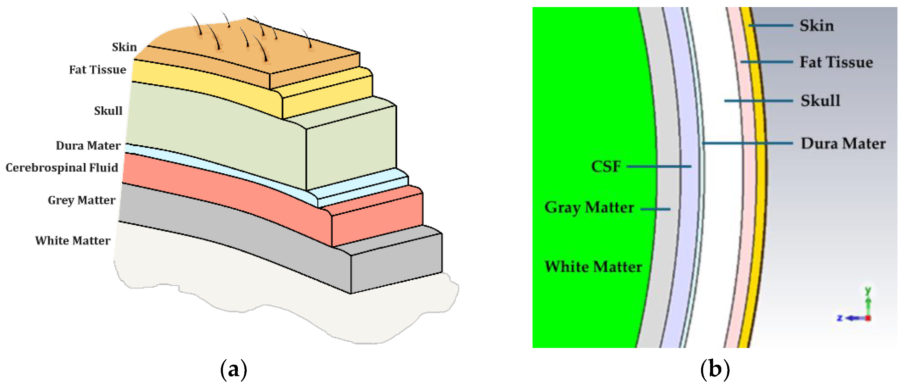
2.1. Human Head Model
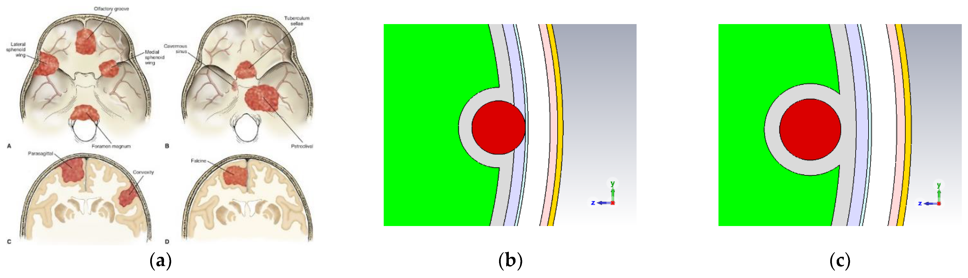
2.2. Meningioma Brain Tumor
3. Ku-Band Antenna Design
3.1. Single-Band Ku-Band Patch Antenna
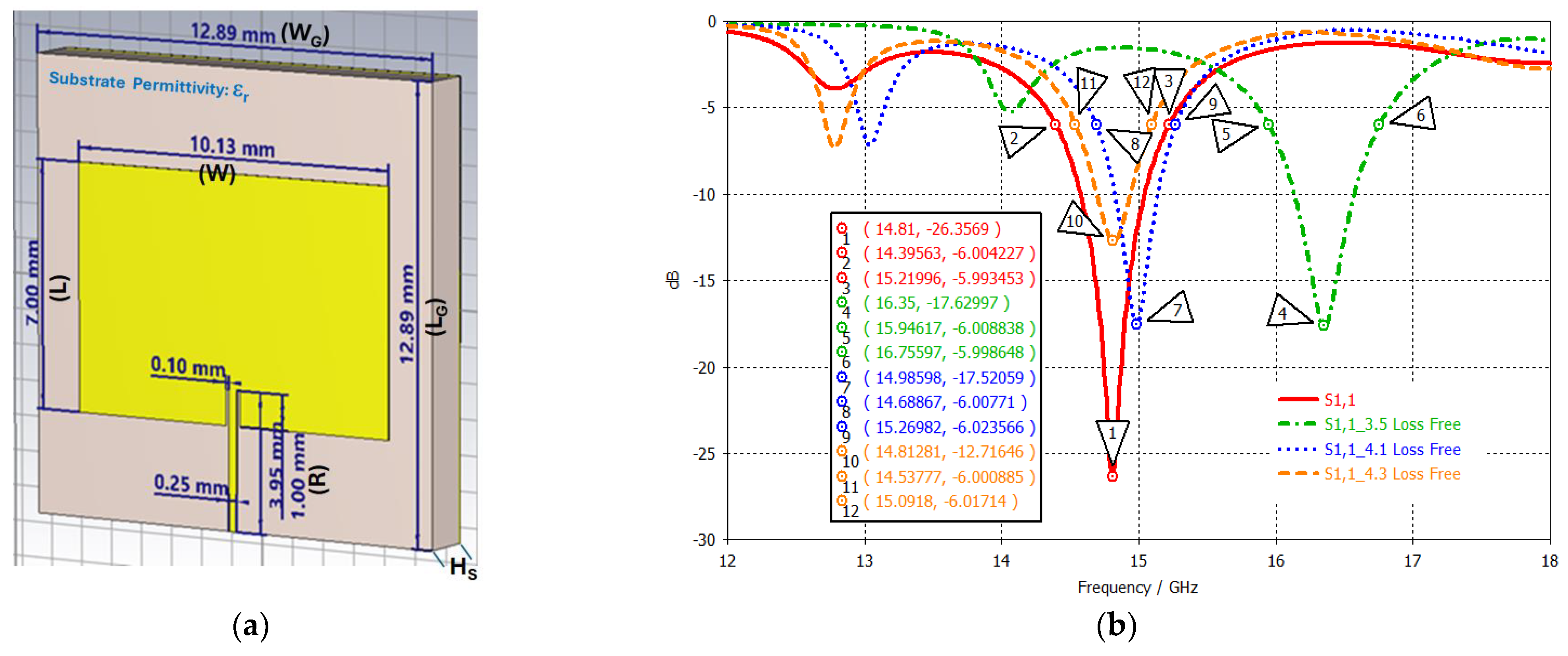
3.1.1. Conventional Rectangular Patch
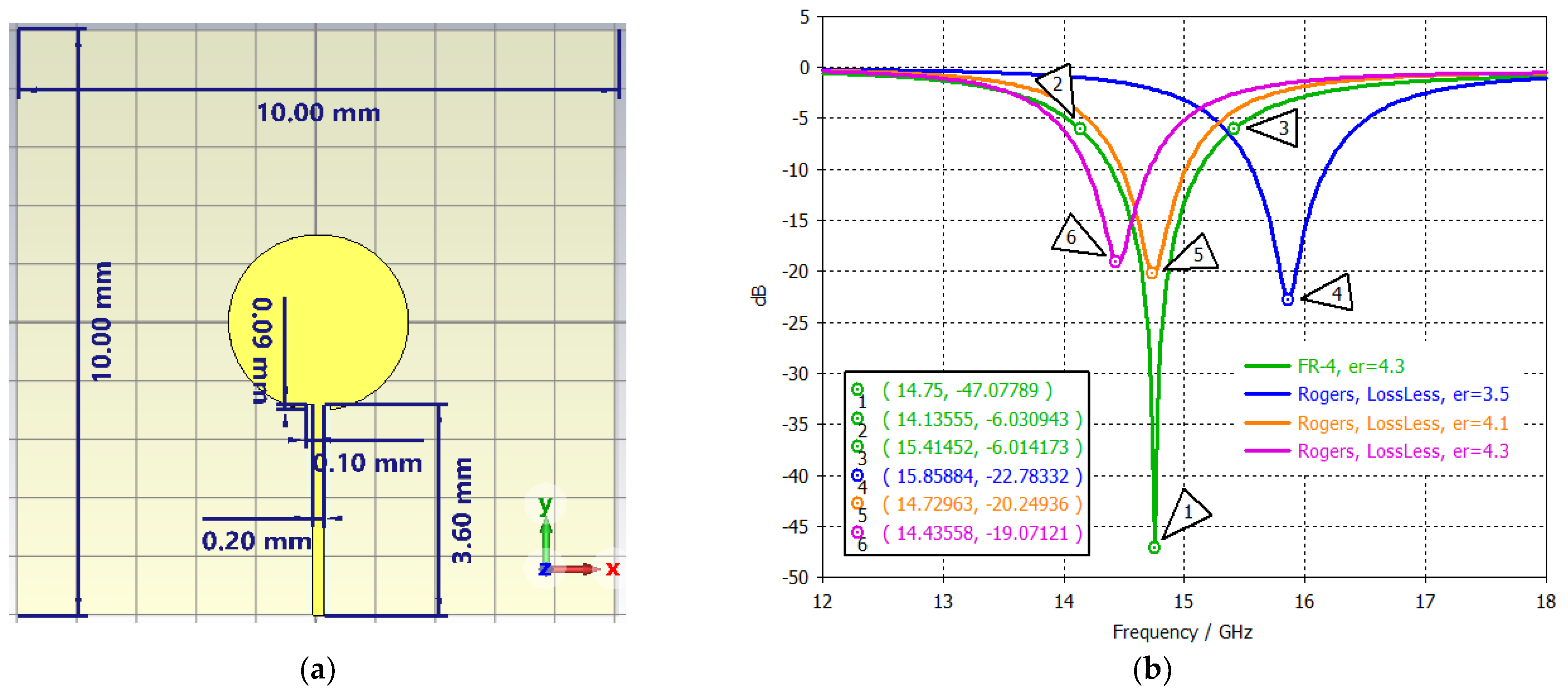
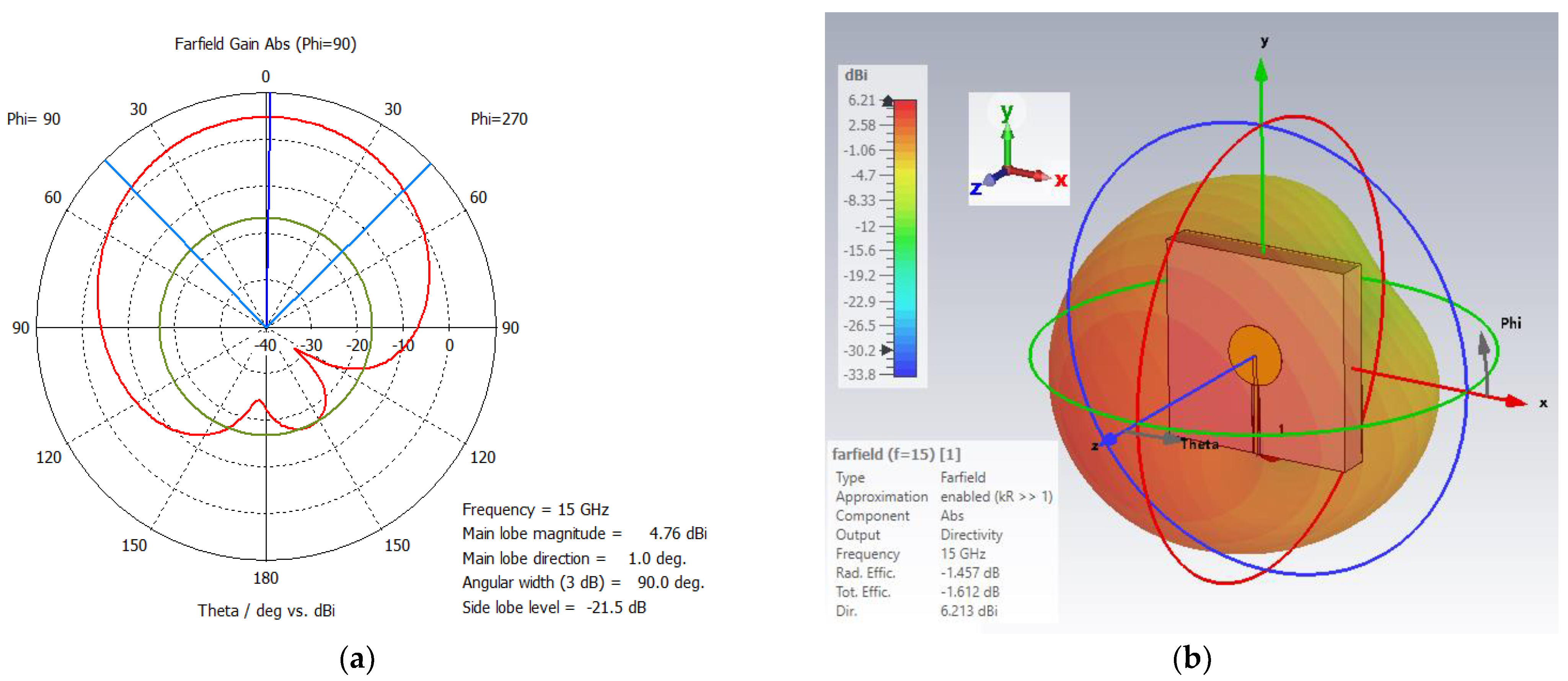
3.1.2. Single–Band Disc Patch
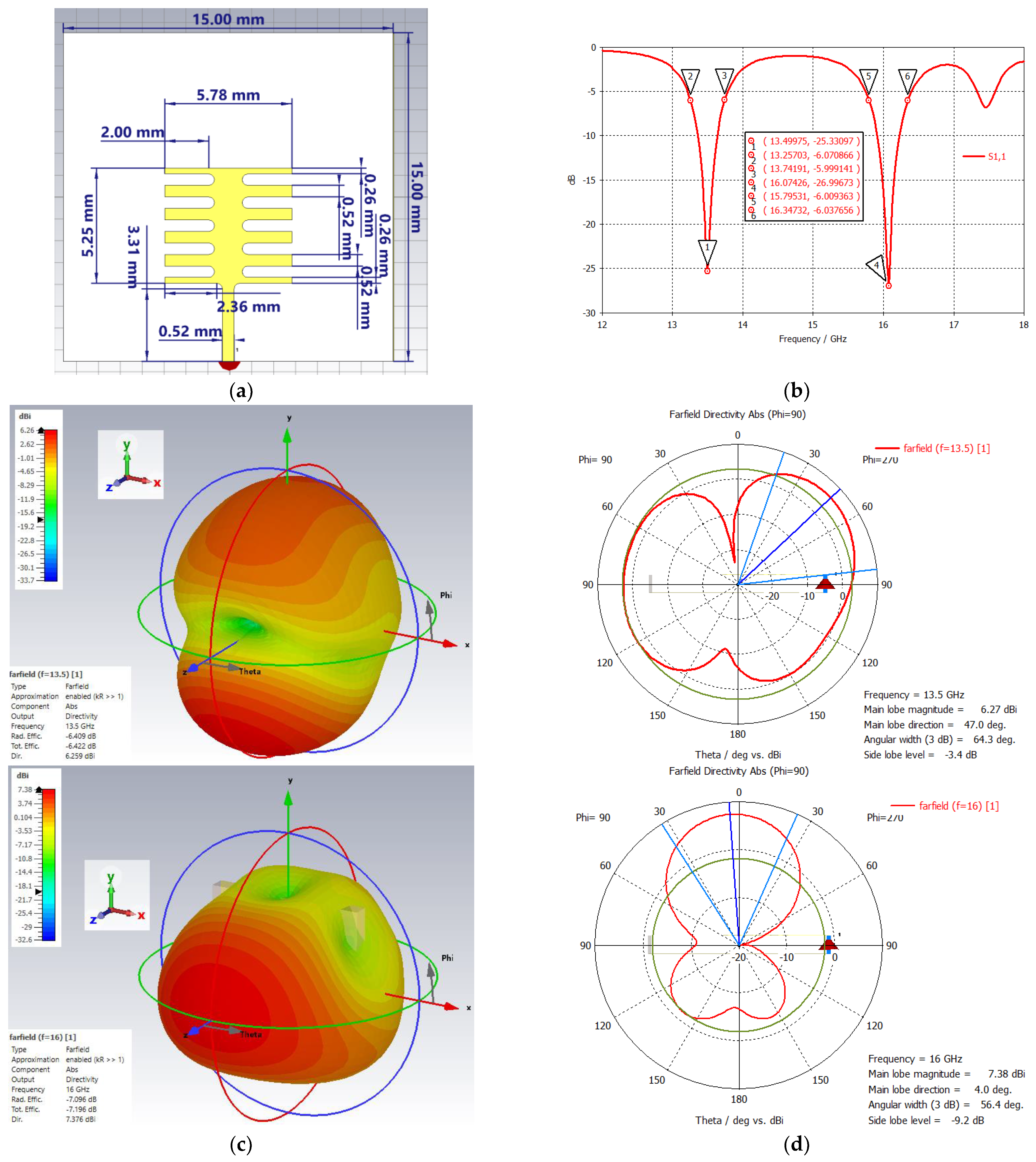
3.2. Dual–Band Metamaterial–Inspired Ku–Band Patch Antenna
3.3. Tri–Band Metamaterial–Inspired Antenna
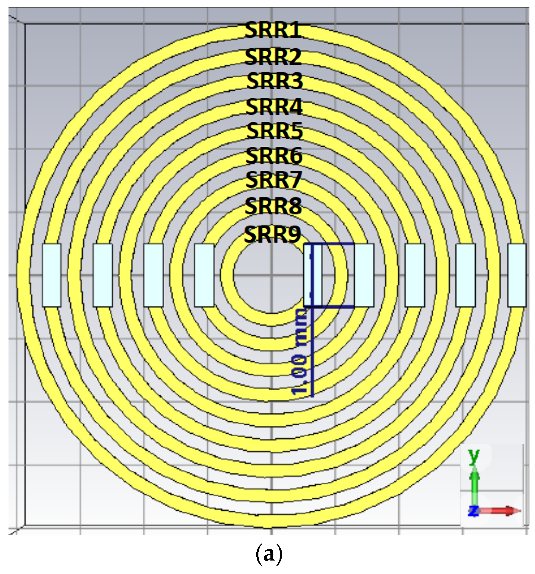
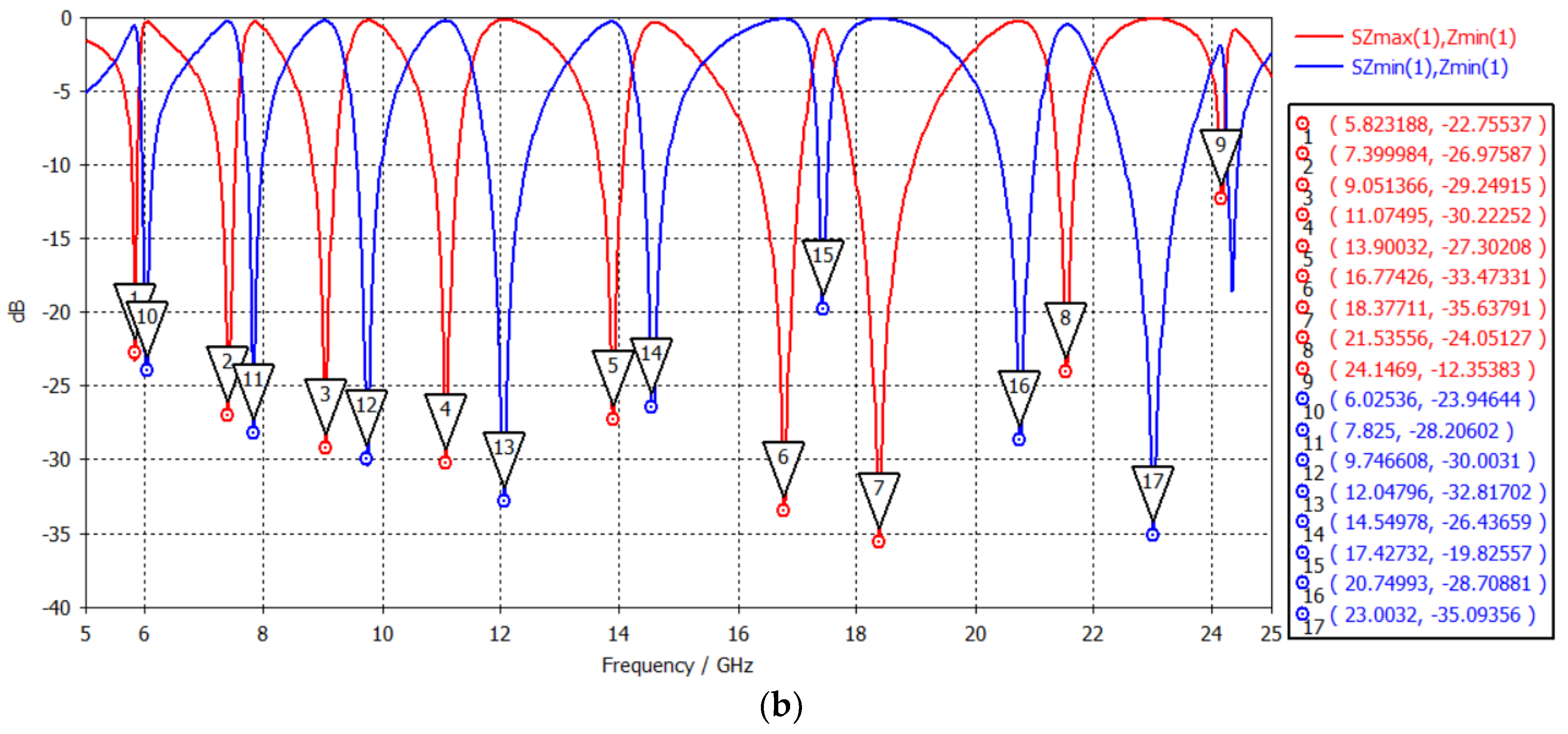
3.3.1. SRR Metamaterial Band Enhancer
3.3.2. Low-Profile Broadband Dipole Antenna
3.3.3. Tri-Band Antenna
4. Brain Tumor Microwave Sensor
4.1. Single-Band Antenna
4.1.1. Rectangular Patch
4.1.2. Disc Patch
4.2. Dual-Band Antenna
4.3. Tri-Band Antenna
5. Conclusions and Discussion
Author Contributions
Funding
Institutional Review Board Statement
Informed Consent Statement
Data Availability Statement
Conflicts of Interest
References
- Brain Tumor Facts. National Brain Tumor Society. Available online: https://braintumor.org/brain-tumors/about-brain-tumors/brain-tumor-facts/ (accessed on 2 July 2024).
- Siegel, R.L.; Miller, K.D.; Wagle, N.S.; Jemal, A. Cancer statistics, 2023. CA Cancer J. Clin. 2023, 73, 17–48. [Google Scholar] [CrossRef] [PubMed]
- Llandro, J.; Palfreyman, J.J.; Ionescu, A.; Barnes, C.H.W. Magnetic biosensor technologies for medical applications: A review. Med. Biol. Eng. Comput. 2010, 48, 977–998. [Google Scholar] [CrossRef] [PubMed]
- Uchiyama, T.; Mohri, K.; Honkura, Y.; Panina, L.V. Recent advances of pico-Tesla resolution magneto-impedance sensor based on amorphous wire CMOS IC MI Sensor. IEEE Trans. Magn. 2012, 48, 3833–3839. [Google Scholar] [CrossRef]
- Melnikov, G.Y.; Lepalovskij, V.N.; Svalov, A.V.; Safronov, A.P.; Kurlyandskaya, G.V. Magnetoimpedance thin film sensor for detecting of stray fields of magnetic particles in blood vessel. Sensors 2021, 21, 3621. [Google Scholar] [CrossRef] [PubMed]
- Raghavendra, U.; Gudigar, A.; Paul, A.; Goutham, T.S.; Inamdar, M.A.; Hegde, A.; Devi, A.; Ooi, C.P.; Deo, R.C.; Barua, P.D.; et al. Brain tumor detection and screening using artificial intelligence techniques: Current trends and future perspectives. Comput. Biol. Med. 2023, 163, 107063. [Google Scholar] [CrossRef]
- Title 47 of the CFR. Available online: https://www.ecfr.gov/current/title-47 (accessed on 10 September 2024).
- IEEE Std C95.3-2021 (Revision of IEEE Std C95.3-2002 and IEEE Std C95.3.1-2010); Recommended Practice for Measurements and Computations of Electric, Magnetic, and Electromagnetic Fields with Respect to Human Exposure to Such Fields, 0 Hz to 300 GHz. IEEE: Piscataway, NJ, USA, 28 May 2021; pp. 1–240. [CrossRef]
- Ahdi Rezaeieh, S.; Zamani, A.; Abbosh, A.M. 3-D Wideband Antenna for Head-Imaging System with Performance Verification in Brain Tumor Detection. IEEE Antennas Wirel. Propag. Lett. 2015, 14, 910–914. [Google Scholar] [CrossRef]
- Saleeb, D.A.; Helmy, R.M.; Areed, N.F.F.; Marey, M.; Abdulkawi, W.M.; Elkorany, A.S. A Technique for the Early Detection of Brain Cancer Using Circularly Polarized Reconfigurable Antenna Array. IEEE Access 2021, 9, 133786–133794. [Google Scholar] [CrossRef]
- Sinha, S.; Niloy, T.-S.R.; Hasan, R.R.; Rahman, M.A.; Rahman, S. A Wearable Microstrip Patch Antenna for Detecting Brain Tumor. In Proceedings of the 2020 International Conference on Computation, Automation and Knowledge Management (ICCAKM), Dubai, United Arab Emirates, 9–10 January 2020; pp. 85–89. [Google Scholar] [CrossRef]
- Chowdhury, T.; Farhin, R.; Hassan, R.R.; Bhuiyan, M.S.A.; Raihan, R. Design of a patch antenna operating at ISM band for brain tumor detection. In Proceedings of the 2017 4th International Conference on Advances in Electrical Engineering (ICAEE), Dhaka, Bangladesh, 28–30 September 2017; pp. 94–98. [Google Scholar] [CrossRef]
- Hossain, A.; Islam, M.T.; Beng, G.K.; Kashem, S.B.A.; Soliman, M.S.; Misran, N.; Chowdhury, M.E.H. Microwave brain imaging system to detect brain tumor using metamaterial loaded stacked antenna array. Sci. Rep. 2022, 12, 16478. [Google Scholar] [CrossRef] [PubMed] [PubMed Central]
- Inum, R.; Rana, M.M.; Shushama, K.N.; Quader, M.A. EBG Based Microstrip Patch Antenna for Brain Tumor Detection via Scattering Parameters in Microwave Imaging System. Int. J. Biomed. Imaging 2018, 2018, 8241438. [Google Scholar] [CrossRef] [PubMed] [PubMed Central]
- Aziz, M.A.I.; Rana, M.M.; Islam, M.A.; Inum, R. Effective Modeling of GBC Based Ultra-Wideband Patch Antenna for Brain Tumor Detection. In Proceedings of the 2018 International Conference on Computer, Communication, Chemical, Material and Electronic Engineering (IC4ME2), Rajshahi, Bangladesh, 8–9 February 2018; pp. 1–4. [Google Scholar] [CrossRef]
- Kordić, A.; Šarolić, A. Dielectric Spectroscopy Shows a Permittivity Contrast between Meningioma Tissue and Brain White and Gray Matter—A Potential Physical Biomarker for Meningioma Discrimination. Cancers 2023, 15, 4153. [Google Scholar] [CrossRef]
- Mobashsher, A.T.; Abbosh, A.M. Artificial Human Phantoms: Human Proxy in Testing Microwave Apparatuses That Have Electromagnetic Interaction with the Human Body. IEEE Microw. Mag. 2015, 16, 42–62. [Google Scholar] [CrossRef]
- CST Microwave Studio. CST Studio Suite. Available online: https://www.3ds.com/products/simulia/cst-studio-suite (accessed on 10 September 2024).
- Adeloye, A.; Kattan, K.R.; Silverman, F.N. Thickness of the normal skull in the American blaacks and whites. Am. J. Biol. Anthropol. 1975, 43, 23–30. [Google Scholar] [CrossRef] [PubMed]
- Hwang, K.; Kim, J.H.; Baik, S.H. The Thickness of the Skull in Korean Adults. J. Craniofac. Surg. 1999, 10, 395–399. [Google Scholar] [CrossRef] [PubMed]
- Lynnerup, N. Cranial thickness in relation to age, sex and general body build in a Danish forensic sample. Forensic Sci. Int. 2001, 117, 45–51. [Google Scholar] [CrossRef] [PubMed]
- Thulung, S.; Ranabhat, K.; Bishokarma, S.; Gongal, D.N. Morphometric Measurement of Cranial Vault Thickness: A Tertiary Hospital Based Study. J. Nepal Med. Assoc. 2019, 57, 29–32. [Google Scholar] [CrossRef] [PubMed]
- Fischl, B.; Dale, A.M. Measuring the thickness of the human cerebral cortex from magnetic resonance images. Biol. Sci. 2000, 97, 11050–11055. [Google Scholar] [CrossRef]
- Gabriel, C. Compilation of the Dielectric Properties of Body Tissues at RF and Microwave Frequencies; Report N.AL/OE-TR-1996-0037; Occupational and Environmental Health Directorate, Radiofrequency Radiation Division: Brooks Air Force Base, TX, USA, 1996. [Google Scholar]
- Brain Tumor Types. John Hopkins Medicine, Health Section. Available online: https://www.hopkinsmedicine.org/health/conditions-and-diseases/brain-tumor/brain-tumor-types (accessed on 7 July 2024).
- Perry, A. 13—Meningiomas. In Practical Surgical Neuropathology: A Diagnostic Approach, 2nd ed.; Perry, A., Brat, D.J., Eds.; Elsevier: Amsterdam, The Netherlands, 2018; pp. 259–298. [Google Scholar] [CrossRef]
- Wongkasem, N.; Ruiz, M. Multi-Negative Index Band Metamaterial-Inspired Microfluidic Sensors. PIER C 2019, 94, 29–44. [Google Scholar] [CrossRef]
- Al-Duhni, G.; Wongkasem, N. Metal discovery by highly sensitive microwave multi-band metamaterial-inspired sensors. Prog. Electromagn. Res. B 2021, 93, 1–22. [Google Scholar] [CrossRef]
- Hassan, K.M.Z.; Wongkasem, N. Development of microwave metamaterial-inspired sensors with multiple-band reactivity for mercury contamination detection. J. Electromagn. Waves Appl. 2022, 36, 520–541. [Google Scholar] [CrossRef]
- Pendry, J.B.; Holden, A.J.; Robbins, D.J.; Stewart, W.J. Magnetism from conductors and enhanced nonlinear phenomena. IEEE Trans. MTT 1999, 47, 2075. [Google Scholar] [CrossRef]
- Katsarakis, N.; Koschny, T.; Kafesaki, M.; Economou, E.N.; Soukoulis, C.M. Electric coupling to the magnetic resonance of split ring resonators. Appl. Phys. Lett. 2004, 84, 2943–2945. [Google Scholar] [CrossRef]
- Kafesaki, M.; Koschny, T.; Penciu, R.S.; Gundogdu, T.F.; Economou, E.N.; Soukoulis, C.M. Left-handed metamaterials: Detailed numerical studies of the transmission properties. J. Opt. A Pure Appl. Opt. 2005, 7, S12. [Google Scholar] [CrossRef]
- Steinberg, K.; Scheffler, M.; Dressel, M. Microwave inductance of thin metal strips. J. Appl. Phys. 2010, 108, 096102. [Google Scholar] [CrossRef]
- Li, H.; Li, S.; Liu, H.; Wang, X. Analysis of electromagnetic scattering from plasmonic inclusions beyond the quasi-static approximation and applications. ESAIM Math. Model. Numer. Anal. 2019, 53, 1351–1371. [Google Scholar] [CrossRef]
- Li, H.; Liu, H. On anomalous localized resonance and plasmonic cloaking beyond the quasistatic limit. Proc. R. Soc. A 2018, 474, 20180165. [Google Scholar] [CrossRef]


| 1. Skin | -Scalp Skin * (1) -Subcutaneous Tissue * (2) -Aponeurosis |
| 2. Skull/Periosteum | -Outer Table/Compact Bone * (3) -Diploe -Inner Table/Compact Bone |
| 3. Meninges | -Dura Mater * (4) [Anatomy of the Cranial and Spinal Meninges] -Endosteal Layer -Meningeal/Fibrous Layer -Neurothelium -Arachnoid Mater -Parietal Arachnoid Layer —Subdural Layer —Central Layer -Subarachnoid Space * (5) -Leptomeningeal Trabeculae (web-like structures) -Cerebrospinal Fluid -Pia Mater -Epipial Layer -Intima Pia/Inner Layer |
| 4. Brain | -Neocortex/Gray Matter * (6) -White Matter * (7) |
| Head Layer | Thickness Range (mm) [11,16,17,18,19,20] | Thickness (mm) [11] | Radius (mm) [11] | |
|---|---|---|---|---|
| 1. | Skin or Epidermis/Dermis | 1.10–3.25 | 1.0 | 90.0 |
| 2. | Fat or Hypodermis/Subcutaneous Tissue | 1.40–7.00 | 1.4 | 89.0 |
| 3. | Bone or Skull | 2.31–9.30 | 4.1 | 87.6 |
| 4. | Dura Mater Tissue | 0.50 | 0.5 | 83.5 |
| 5. | Subarachnoid Space/ Cerebrospinal Fluid (CSF) | 0.44–2.40 | 2.0 | 83.0 |
| 6. | Gray Matter | 2.50 | 2.5 | 81.0 |
| 7 | White Matter | 78.50 | 78.5 | 78.5 |
| Layer | Electric Dispersive Properties |
|---|---|
1. Skin or Epidermis/Dermis |  |
2. Fat or Hypodermis/Subcutaneous Tissue |  |
3. Bone or Skull |  |
4. Dura Mater Tissue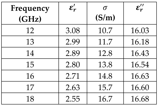 | 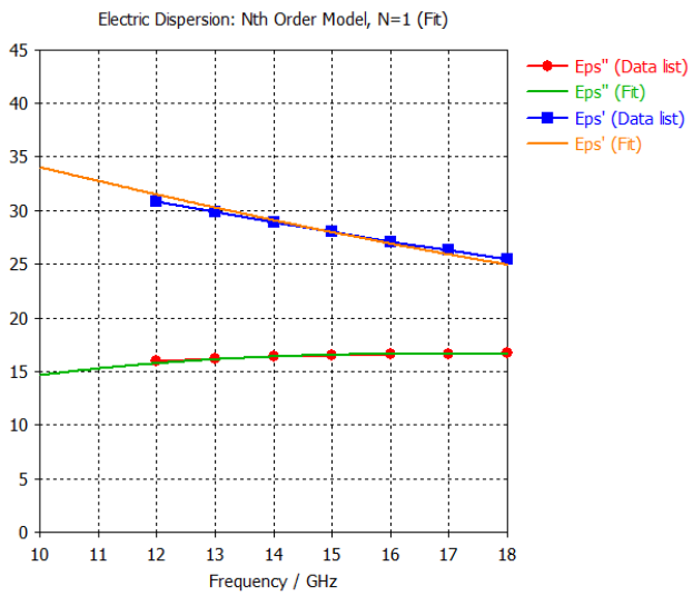 |
5. Subarachnoid Space/Cerebrospinal Fluid (CSF) |  |
6. Gray Matter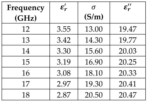 | 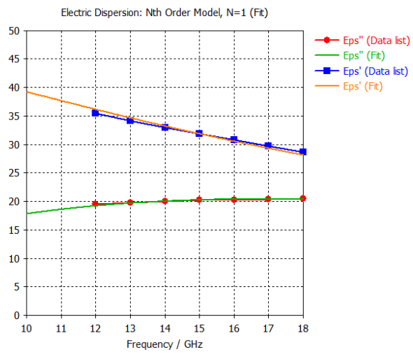 |
7. White Matter |  |
| Patch Length | L | 7.00 mm | Ground Length | LG | 12.89 mm |
| Patch Width | W | 10.13 mm | Ground Width | WG | 12.89 mm |
| Inset Length | LI | 1.00 mm | Cu Thickness (1 oz) | HM | 0.035 mm |
| Inset Width | WI | 0.10 mm | Substrate Thickness (Height) | Hs | 1.50 mm |
| Feed Length | LF | 3.95 mm | |||
| Feed Width | WF | 0.25 mm |
| Substrate | BW% | Gain at 14.8 GHz (dBi) | Gain at 15.0 GHz (dBi) |
|---|---|---|---|
| FR-4, | 5.54 | 1.782 | 2.039 |
| Rogers 410, | 3.87 | 3.958 | 4.331 |
| Rogers 430, | 3.71 | 4.485 | 4.764 |
| Resonance | S11 | S21 |
|---|---|---|
| 1 | 6.03 GHz/−23.95 dB | 5.82 GHz/−22.76 dB |
| 2 | 7.83 GHz/−28.21 dB | 7.40 GHz/−26.98 dB |
| 3 | 9.75 GHz/−30.00 dB | 9.05 GHz/−29.25 dB |
| 4 | 12.05 GHz/−32.82 dB | 11.07 GHz/−30.22 dB |
| 5 | 14.55 GHz/−26.44 dB | 13.90 GHz/−27.30 dB |
| 6 | 17.43 GHz/−19.83 dB | 16.77 GHz/−33.47 dB |
| 7 | 20.75 GHz/−28.71 dB | 18.38 GHz/−35.64 dB |
| 8 | 23.00 GHz/−35.09 dB | 21.54 GHz/−24.05 dB |
| 9 | - | 24.15 GHz/−12.35 dB |
| # | Tumor Diameter (mm) | Frequency (GHz) | S11 (dB) |
|---|---|---|---|
| No Tumor | 15.1684 | −39.4112 | |
| 1 | 2 | 15.1695 | −40.9031 |
| 2 | 4 | 15.1790 | −37.9046 |
| 3 | 6 | 15.1703 | −39.4733 |
| 4 | 8 | 15.1658 | −39.4792 |
| 5 | 10 | 15.1758 | −37.7204 |
| 6 | 12 | 15.1575 | −41.7402 |
| 7 | 14 | 15.1719 | −38.7485 |
| 8 | 16 | 15.1831 | −37.2366 |
| 9 | 18 | 15.1798 | −37.7878 |
| 10 | 20 | 15.1923 | −36.0647 |
| # | Tumor Diameter (mm) | Frequency (GHz) | S11 (dB) |
|---|---|---|---|
| No Tumor | 14.5002 | −35.6476 | |
| 1 | 2 | 14.4869 | −36.6056 |
| 2 | 4 | 14.5083 | −35.4346 |
| 3 | 6 | 14.4645 | −38.7742 |
| 4 | 8 | 14.4802 | −36.4792 |
| 5 | 10 | 14.4886 | −36.0421 |
| 6 | 12 | 14.4822 | −36.4104 |
| 7 | 14 | 14.5070 | −35.7471 |
| 8 | 16 | 14.4890 | −36.5539 |
| 9 | 18 | 14.5147 | −34.8586 |
| 10 | 20 | 14.5097 | −35.2539 |
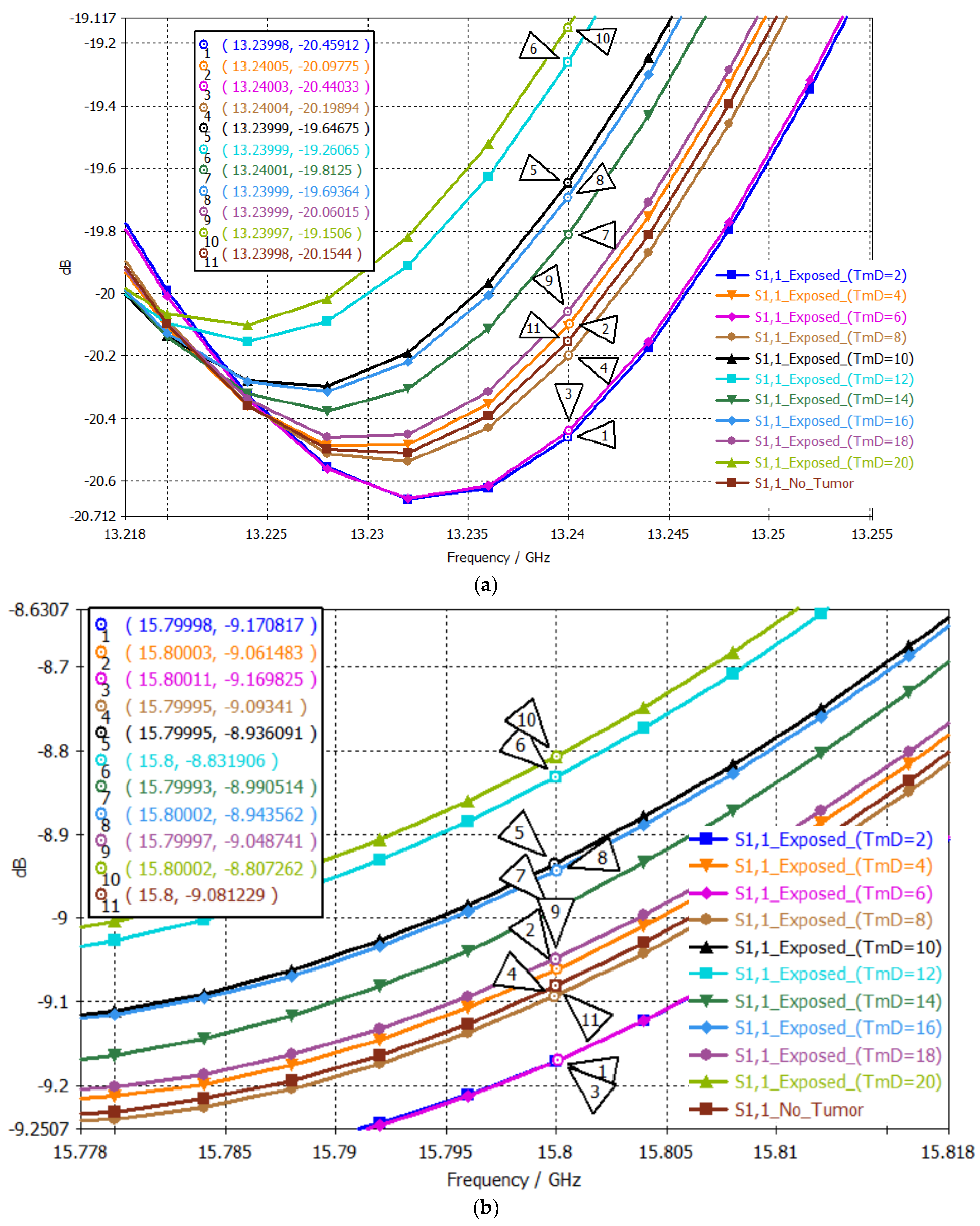
| # | Tumor Diameter (mm) | S11 (dB) at 13.24 GHz 1st Passband | Order 1st Point | S11 (dB) at 15.80 GHz 2nd Passband | Order 1st Point | Two-Point Mapping |
|---|---|---|---|---|---|---|
| No Tumor | −20.1544 | 8 | −9.0812 | 8 | 8-8 | |
| 1 | 2 | −20.4591 | 11 | −9.1712 | 11 | 11-11 |
| 2 | 4 | −20.0978 | 7 | −9.0614 | 7 | 7-7 |
| 3 | 6 | −20.4403 | 10 | −9.1698 | 10 | 10-10 |
| 4 | 8 | −20.1989 | 9 | −9.0934 | 9 | 9-9 |
| 5 | 10 | −19.6468 | 3 | −8.9361 | 3 | 3-3 |
| 6 | 12 | −19.2607 | 2 | −8.8319 | 2 | 2-2 |
| 7 | 14 | −19.8125 | 5 | −8.9905 | 5 | 5-5 |
| 8 | 16 | −19.6936 | 4 | −8.9436 | 4 | 4-4 |
| 9 | 18 | −20.0601 | 6 | −9.0487 | 6 | 6-6 |
| 10 | 20 | −19.1506 | 1 | −8.8073 | 1 | 1-1 |
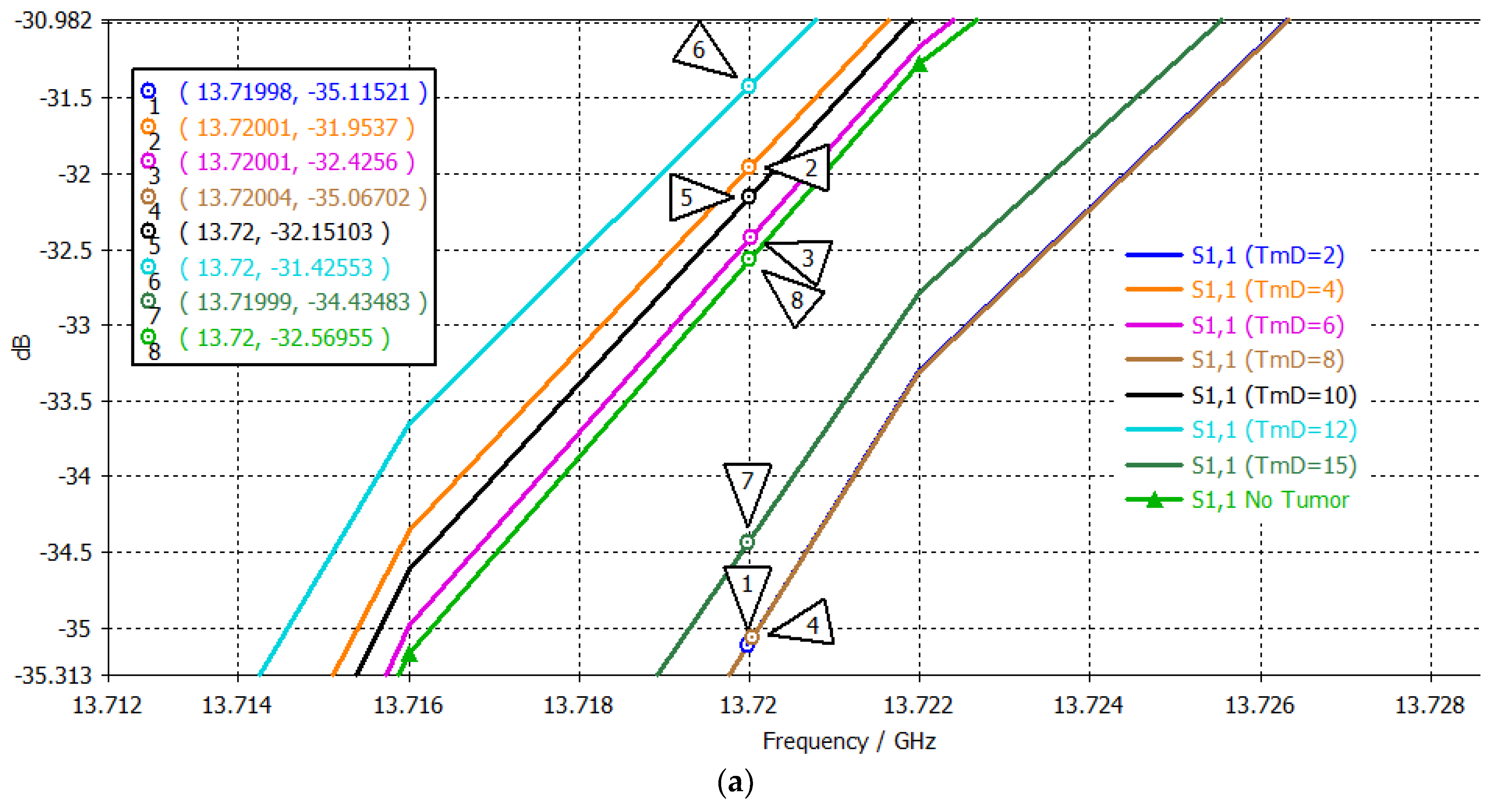
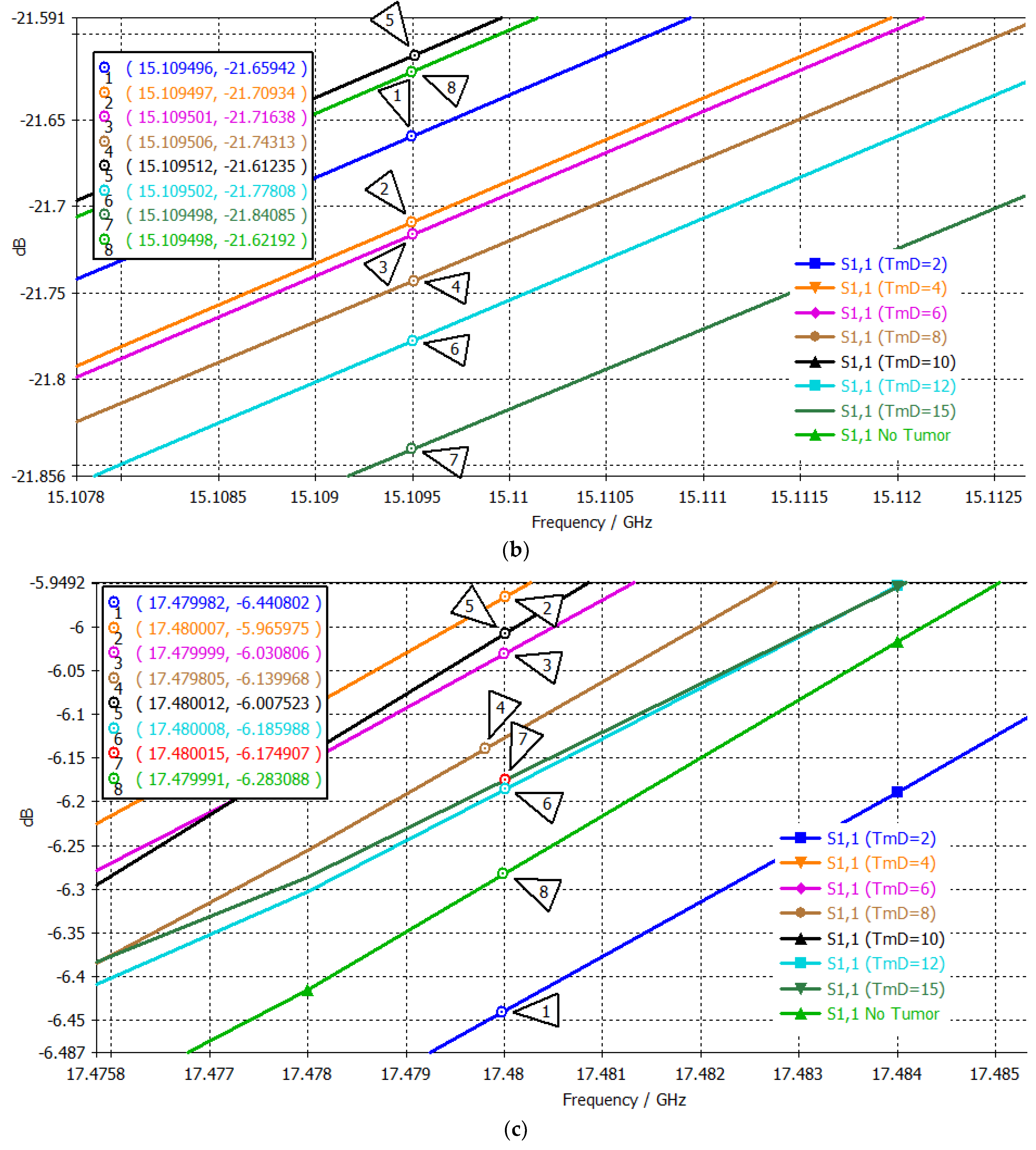
| # | Tumor Diameter (mm) | S11 (dB) at 13.72 GHz 1st Passband | Order 1st Point | S11 (dB) at 15.1095 GHz 2nd Passband | Order 2nd Point | S11 (dB) at 17.48 GHz 3rd Passband | Order 3rd Point | Three-Point Mapping |
|---|---|---|---|---|---|---|---|---|
| No Tumor | −32.5696 | 5 | −21.6219 | 2 | −6.2831 | 7 | 5-2-7 | |
| 1 | 2 | −35.1152 | 8 | −21.6594 | 3 | −6.4408 | 8 | 8-3-8 |
| 2 | 4 | −31.9537 | 2 | −21.7093 | 4 | −5.9660 | 1 | 2-4-1 |
| 3 | 6 | −32.4256 | 4 | −21.7164 | 5 | −6.0308 | 3 | 4-5-3 |
| 4 | 8 | −35.0670 | 7 | −21.7431 | 6 | −6.1400 | 4 | 7-6-4 |
| 5 | 10 | −32.1510 | 3 | −21.6124 | 1 | −6.0075 | 2 | 3-1-2 |
| 6 | 12 | −31.4255 | 1 | −21.7781 | 7 | −6.1860 | 6 | 1-7-6 |
| 7 | 15 | −34.4348 | 6 | −21.8409 | 8 | −6.1749 | 5 | 6-8-5 |
Disclaimer/Publisher’s Note: The statements, opinions and data contained in all publications are solely those of the individual author(s) and contributor(s) and not of MDPI and/or the editor(s). MDPI and/or the editor(s) disclaim responsibility for any injury to people or property resulting from any ideas, methods, instructions or products referred to in the content. |
© 2024 by the authors. Licensee MDPI, Basel, Switzerland. This article is an open access article distributed under the terms and conditions of the Creative Commons Attribution (CC BY) license (https://creativecommons.org/licenses/by/4.0/).
Share and Cite
Wongkasem, N.; Cabrera, G. Multiple-Point Metamaterial-Inspired Microwave Sensors for Early-Stage Brain Tumor Diagnosis. Sensors 2024, 24, 5953. https://doi.org/10.3390/s24185953
Wongkasem N, Cabrera G. Multiple-Point Metamaterial-Inspired Microwave Sensors for Early-Stage Brain Tumor Diagnosis. Sensors. 2024; 24(18):5953. https://doi.org/10.3390/s24185953
Chicago/Turabian StyleWongkasem, Nantakan, and Gabriel Cabrera. 2024. "Multiple-Point Metamaterial-Inspired Microwave Sensors for Early-Stage Brain Tumor Diagnosis" Sensors 24, no. 18: 5953. https://doi.org/10.3390/s24185953
APA StyleWongkasem, N., & Cabrera, G. (2024). Multiple-Point Metamaterial-Inspired Microwave Sensors for Early-Stage Brain Tumor Diagnosis. Sensors, 24(18), 5953. https://doi.org/10.3390/s24185953