
Fault Diagnosis in Wind Turbine Current Sensors: Detecting Single and Multiple Faults with the Extended Kalman Filter Bank Approach


Abstract
1. Introduction
- -
- The proposed approach is capable of identifying current sensor faults in both converters in the three-phase reference frame (a, b, c).
- -
- The diagnostic algorithm is based on the estimation and prediction of currents using a nonlinear and linear Kalman filter with a logic combination block.
- -
- The nonlinearity problem in our system is solved by Jacobi’s discrete-time method.
- -
- The developed fault diagnosis technique is applied for RSC and GSC current sensors based on the EKF.
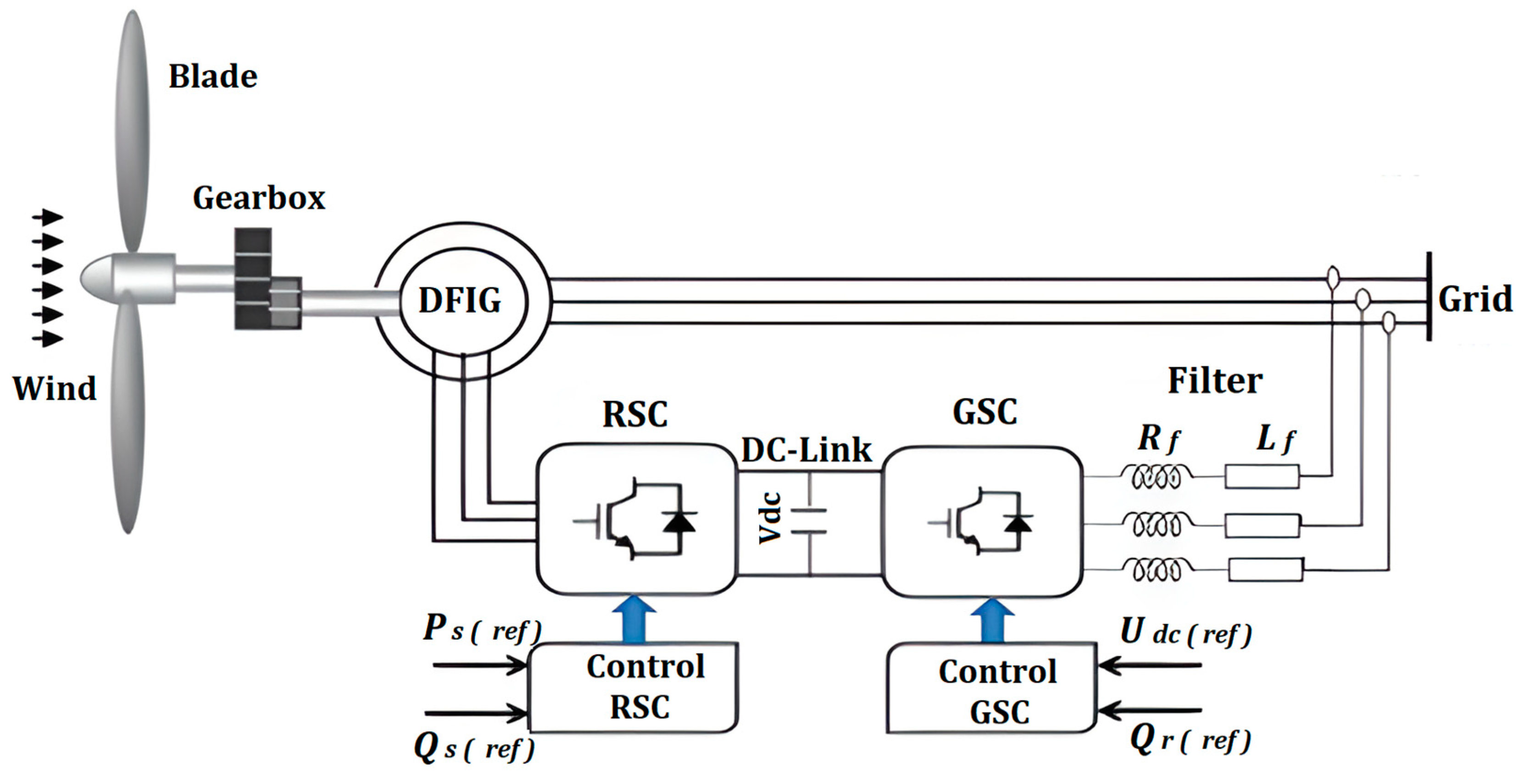
2. Wind Power System Modelling
2.1. DFIG Modeling
2.2. Modeling of the GSC Connection
3. The Sensor Fault Diagnosis Approach
3.1. Fault Detection
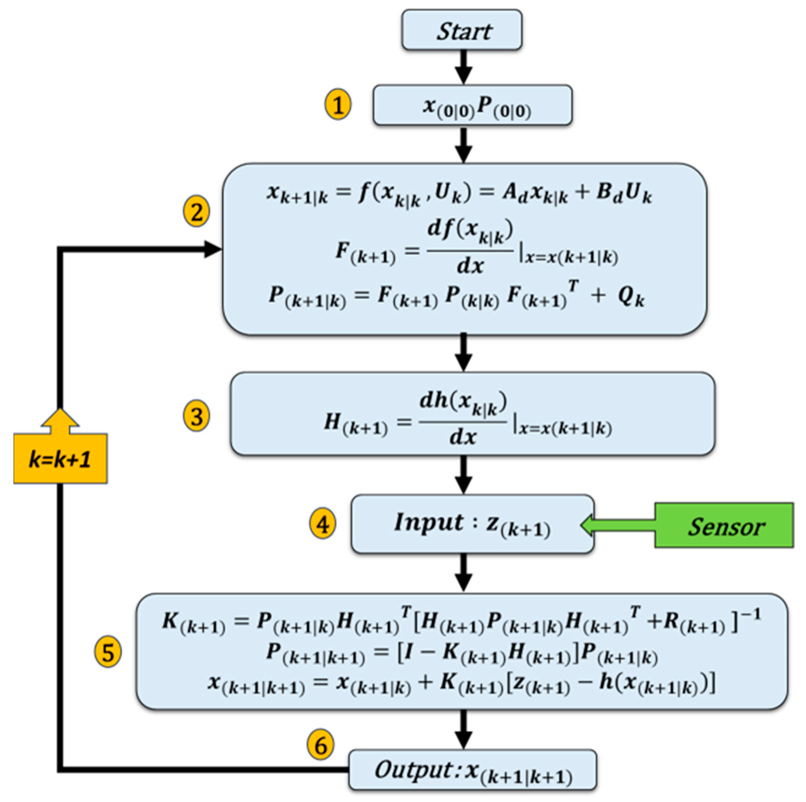
3.1.1. EKF Application on the RSC
- Initialization step: calculates the initial state vector at time k = 0 and the covariance matrix associated with the initially estimated state.
- The prediction phase: calculates the system state, the Jacobian of the nonlinear matrix F with respect to the state variables x and the covariance matrix.
- Calculate the Jacobian of the nonlinear matrix H with respect to the state variables x.
- Acquisition of a new current measurement.
- Update phase: Kalman gain calculation, estimate update, covariance matrix update.
- Estimated state variables used.
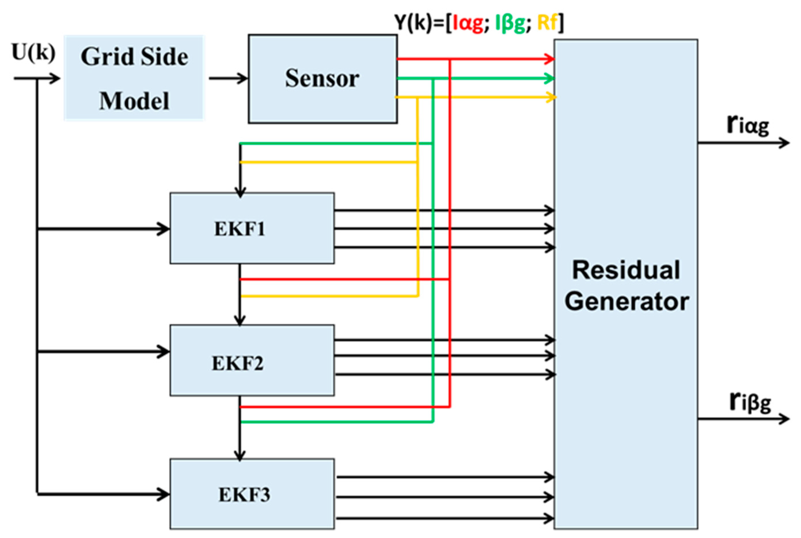
3.1.2. EKF Application on the GSC
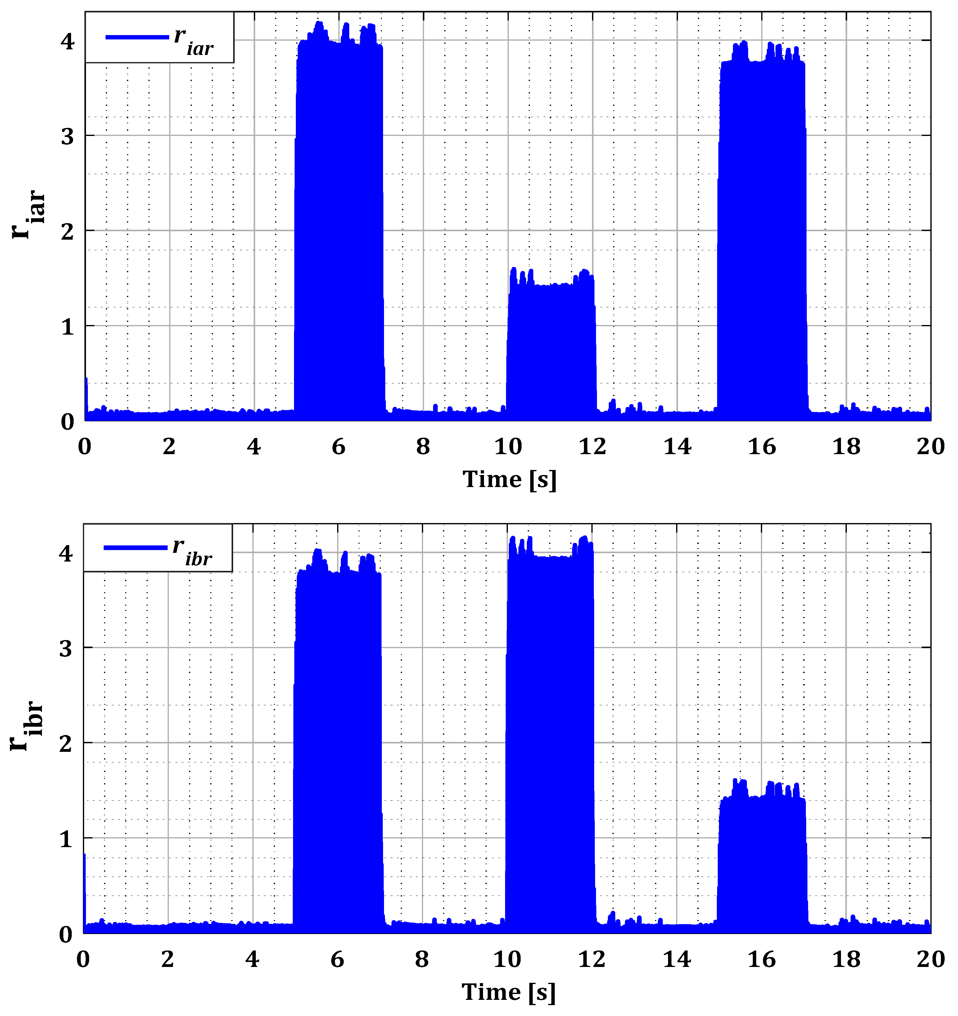
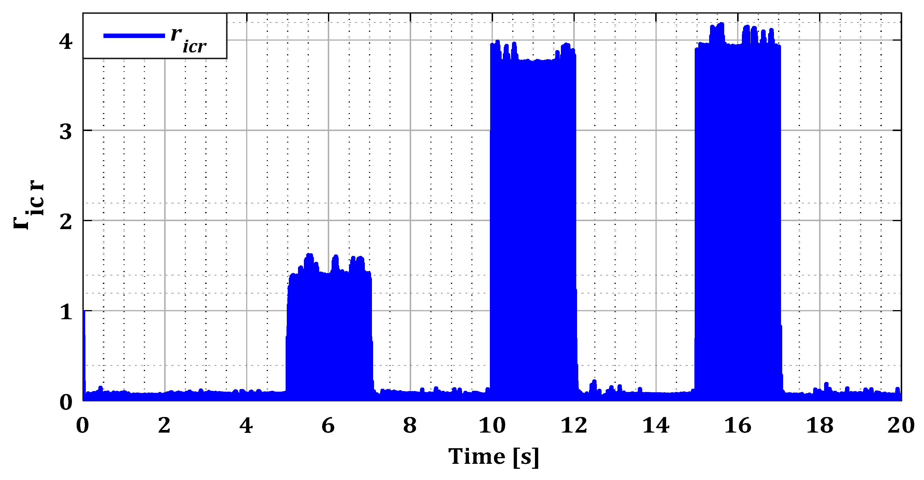
3.2. Localization and Isolation
- If and fault on sensor a; x = [1 0 0].
- If and fault on sensor b; x = [0 1 0].
- If and fault on sensor c; x = [0 0 1].
- If and fault on sensor a and b; x = [1 1 0].
- If and fault on sensor a and c; x = [1 0 1].
- If and fault on sensor b and c; x = [0 1 1].
- If and fault on sensor a, b and c; x = [1 1 1].
- If and x = [0 0 0].with:j = r: for the RSC.and:j = f: for GSC.
3.3. Decision
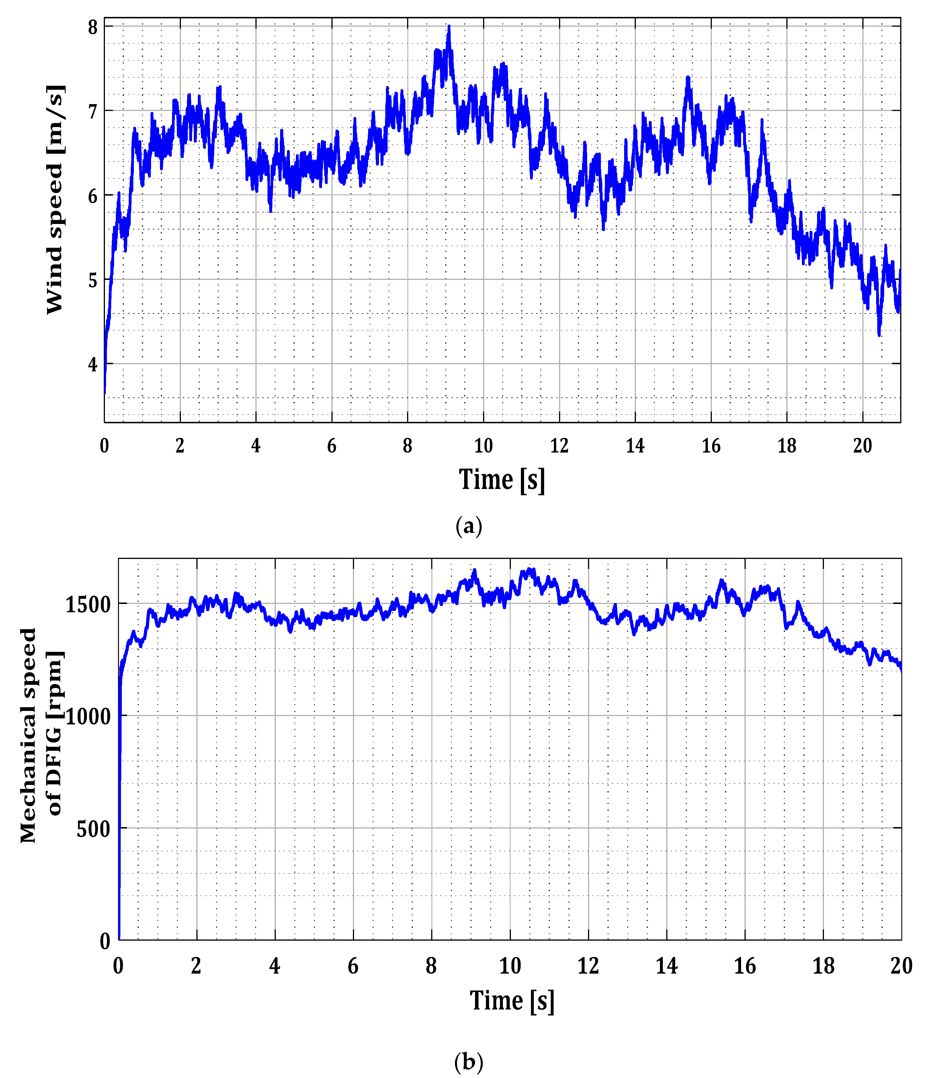
4. Test Results
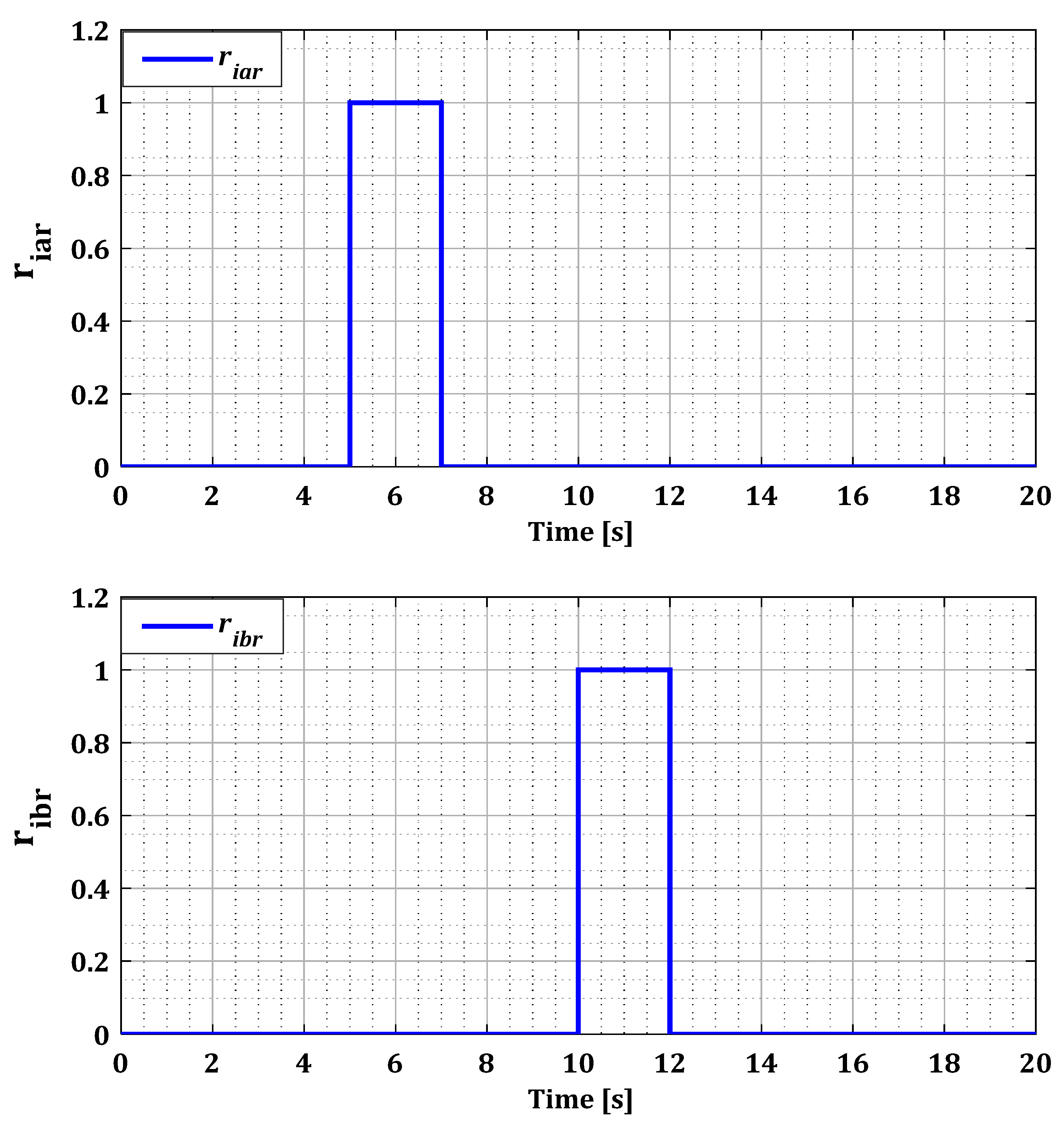
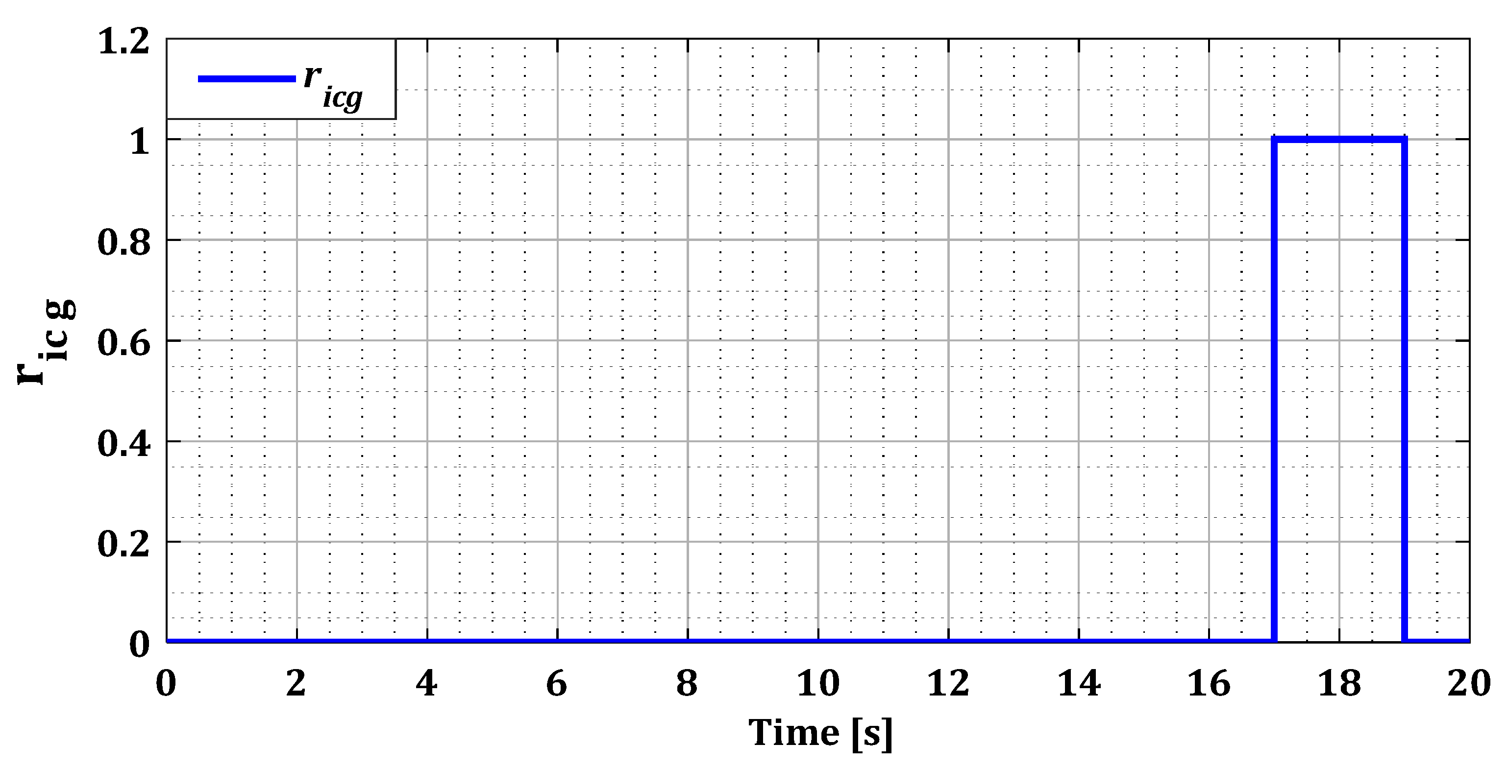
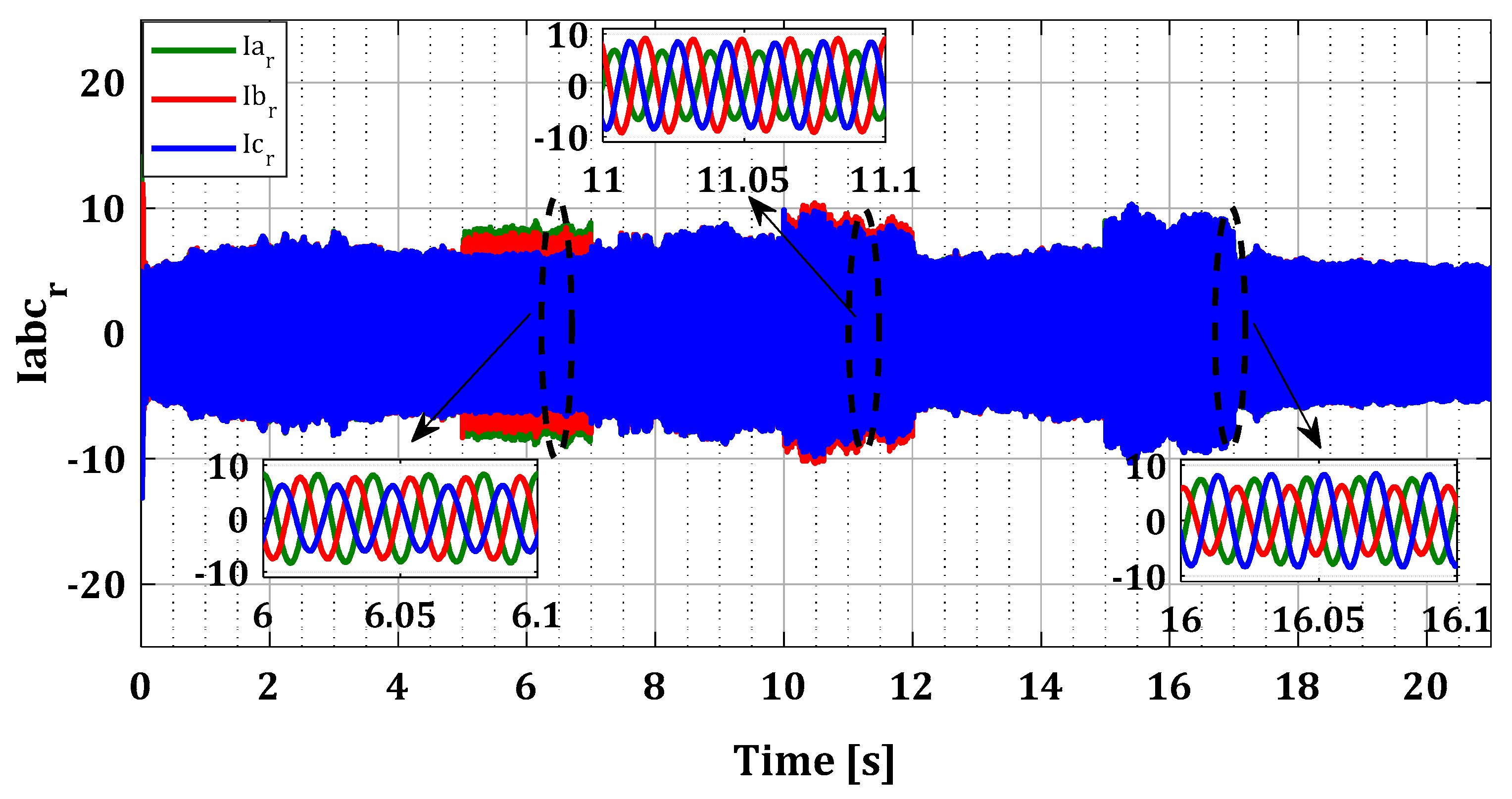
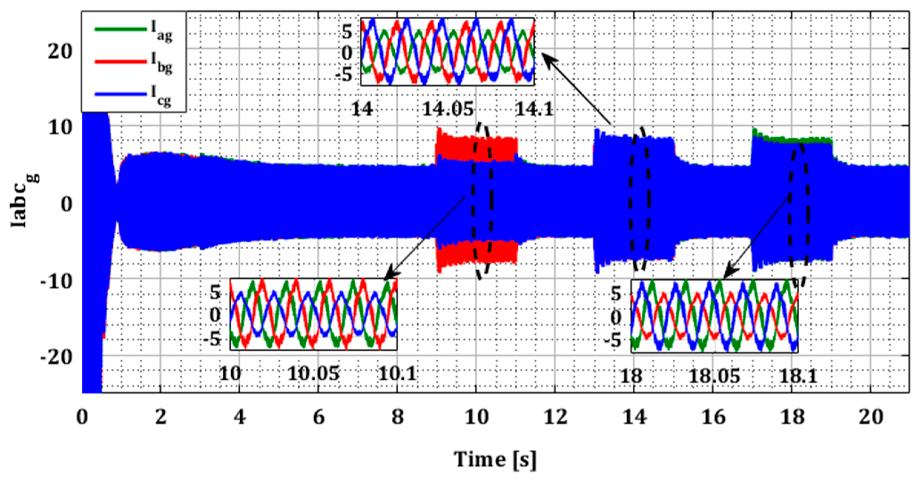
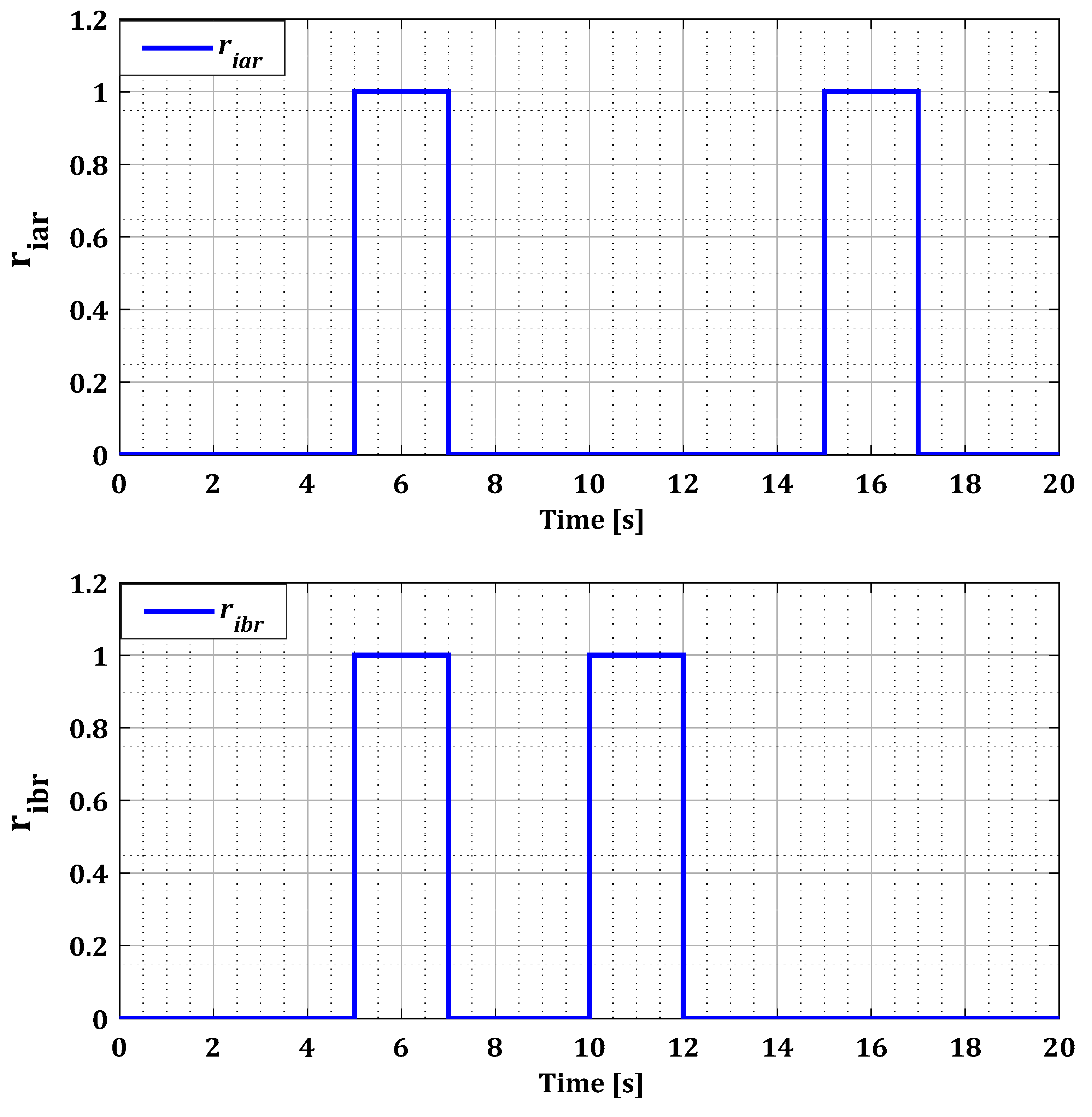
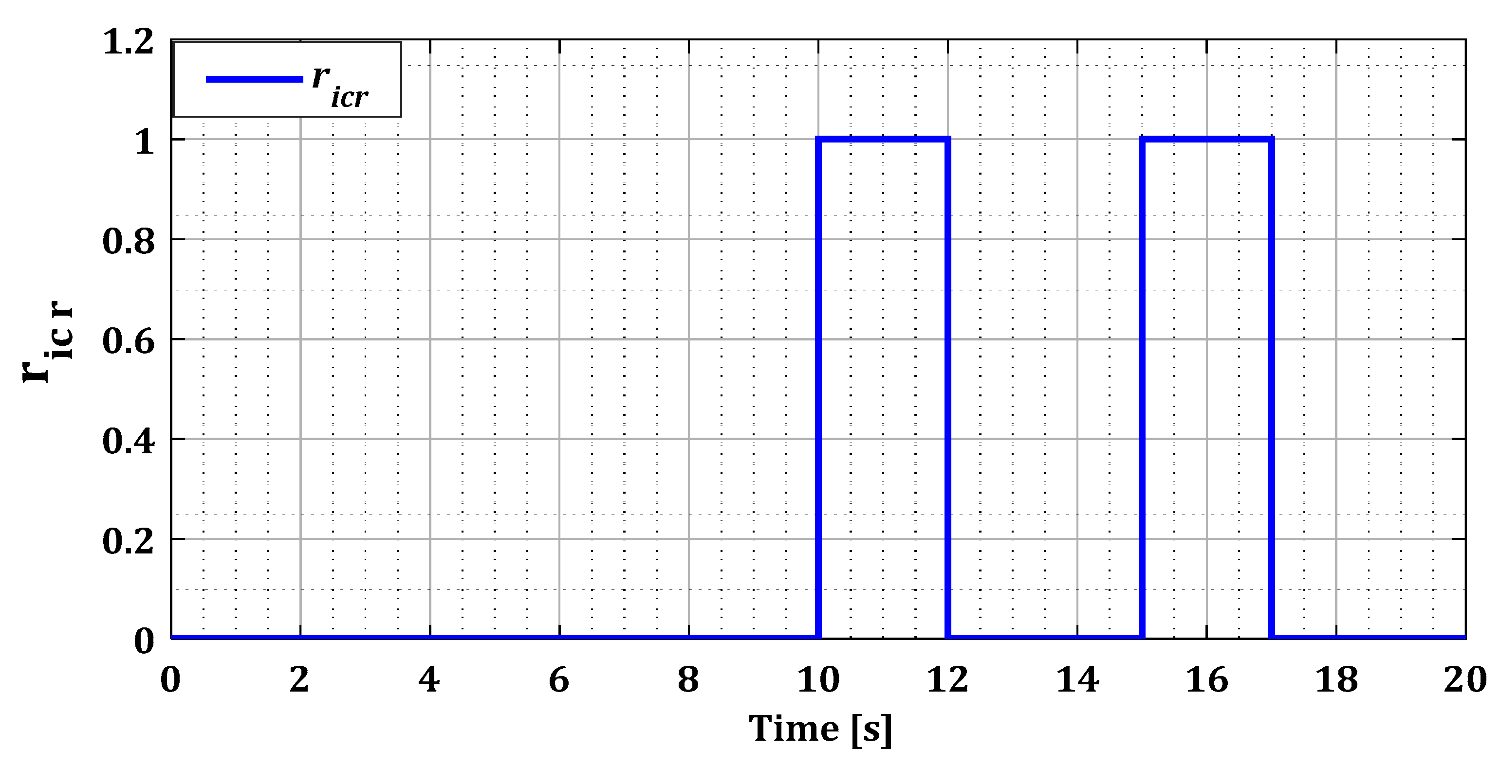
4.1. Scenario of Unique Defects
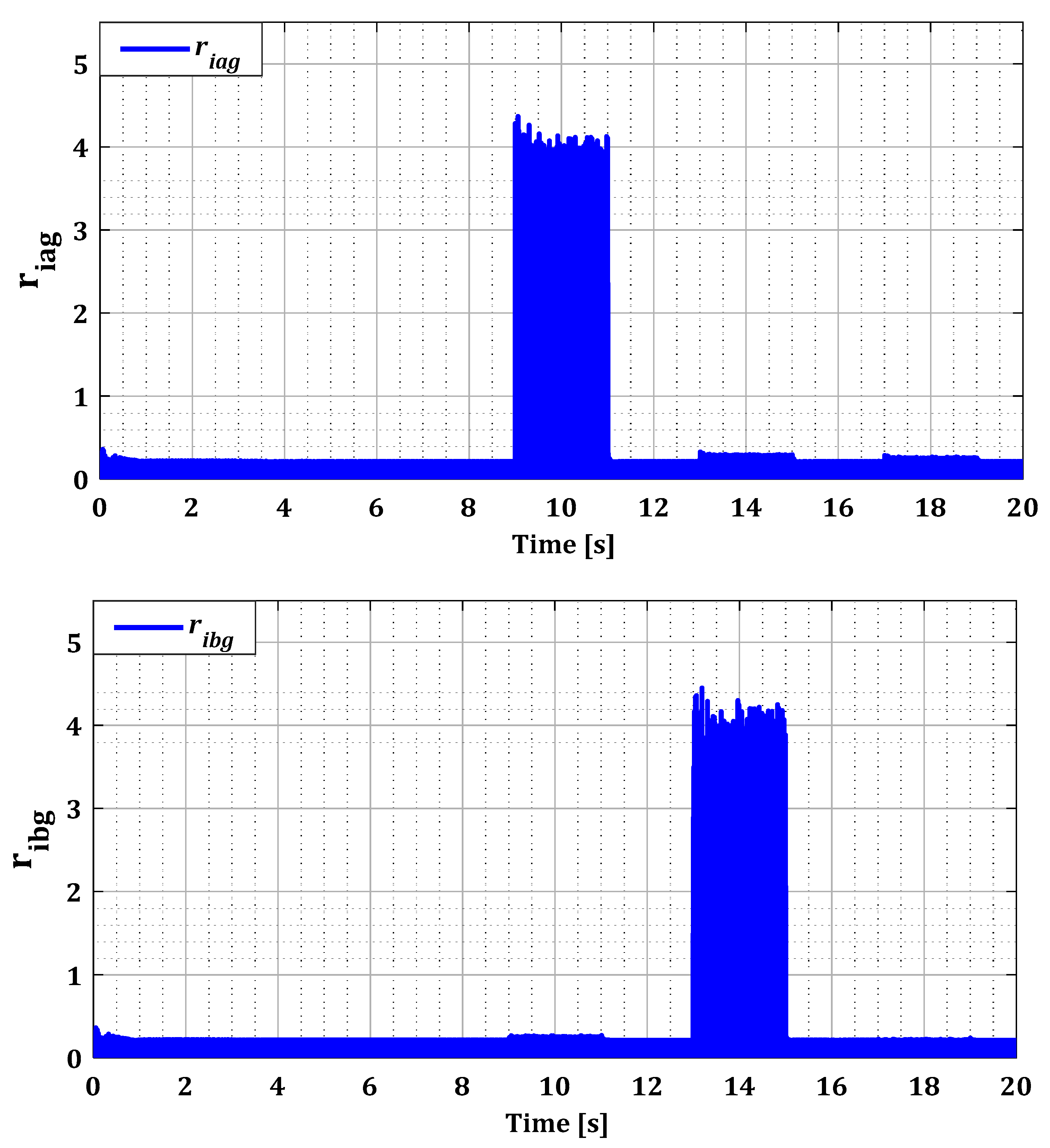
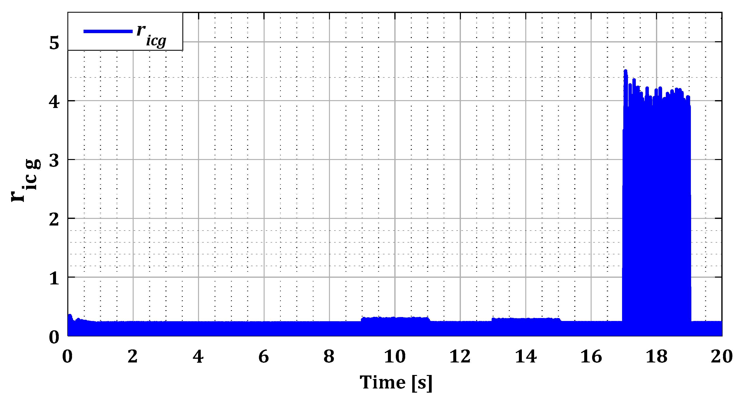
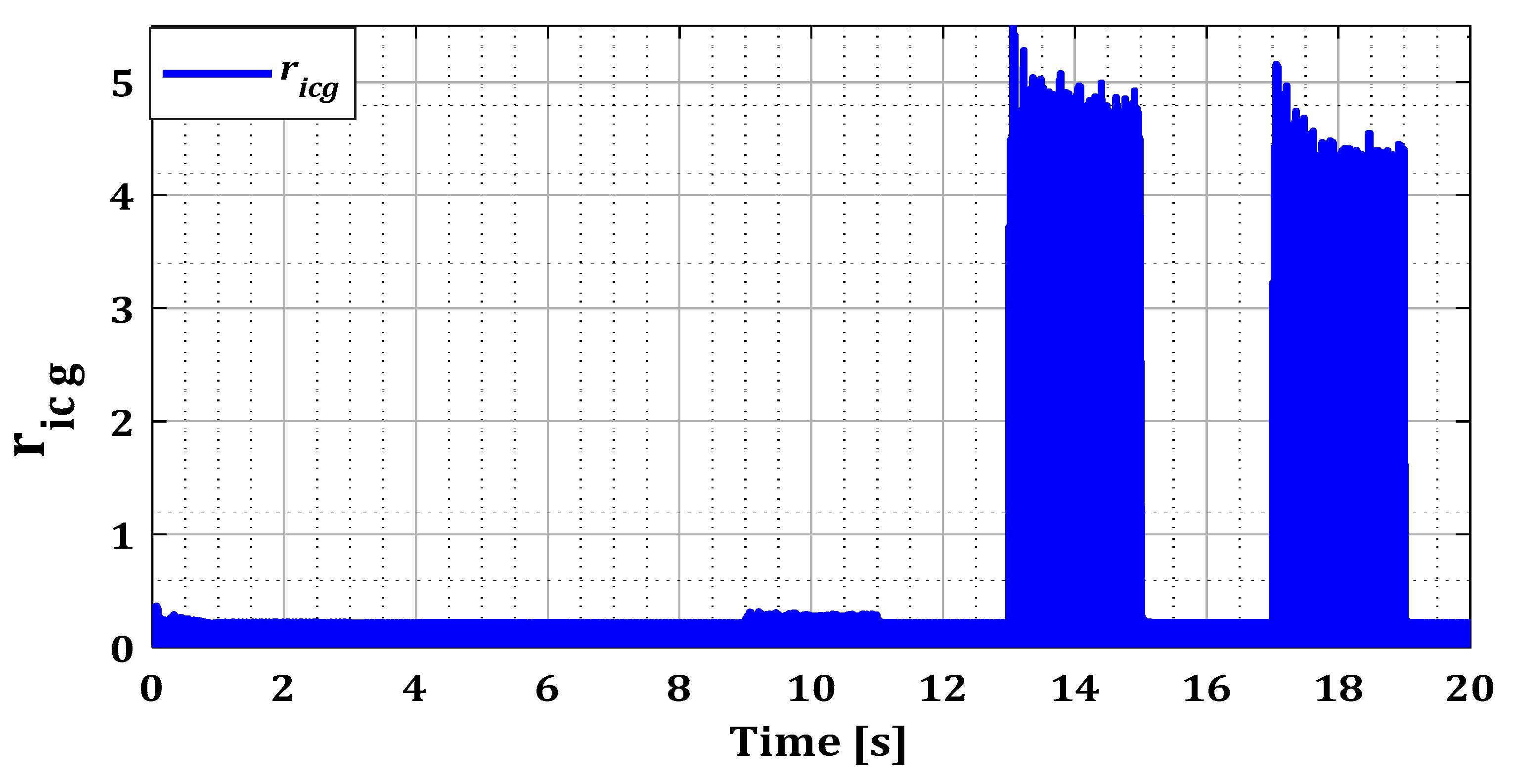
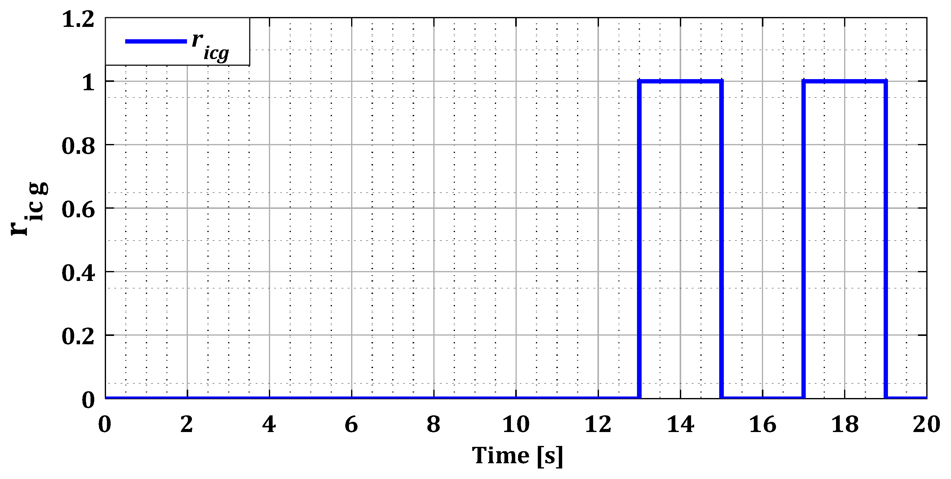
4.2. Multiple Faults Scenario
5. Conclusions
Author Contributions
Funding
Institutional Review Board Statement
Informed Consent Statement
Data Availability Statement
Conflicts of Interest
References
- Mahmoud, M.M.; Atia, B.S.; Esmail, Y.M.; Ardjoun, S.A.E.M.; Anwer, N.; Omar, A.I.; Alsaif, F.; Alsulamy, S.; Mohamed, S.A. Application of Whale Optimization Algorithm Based FOPI Controllers for STATCOM and UPQC to Mitigate Harmonics and Voltage Instability in Modern Distribution Power Grids. Axioms 2023, 12, 420. [Google Scholar] [CrossRef]
- Ardjoun, S.A.E.M.; Denaï, M.; Chafouk, H. A Robust Control Approach for Frequency Support Capability of Grid-Tie Photovoltaic Systems. J. Sol. Energy Eng. 2022, 145, 021009. [Google Scholar] [CrossRef]
- Gholamian, M.; Beik, O. Coordinate Control of Wind Turbines in a Medium Voltage DC Grid. IEEE Trans. Ind. Appl. 2023, 59, 6480–6488. [Google Scholar] [CrossRef]
- Avila, D.; Marichal, G.N.; Hernández, Á.; San Luis, F. Hybrid renewable energy systems for energy supply to autonomous desalination systems on Isolated Islands. In Design, Analysis, and Applications of Renewable Energy Systems; Elsevier: Amsterdam, The Netherlands, 2021; pp. 23–51. [Google Scholar] [CrossRef]
- Boudjemai, H.; Ardjoun, S.A.E.M.; Chafouk, H.; Denaï, M.; Alkuhayli, A.; Khaled, U.; Mahmoud, M.M. Experimental Analysis of a New Low Power Wind Turbine Emulator Using a DC Machine and Advanced Method for Maximum Wind Power Capture. IEEE Access 2023, 11, 92225–92241. [Google Scholar] [CrossRef]
- Li, Y.; Shen, X. Anomaly Detection and Classification Method for Wind Speed Data of Wind Turbines Using Spatiotemporal Dependency Structure. IEEE Trans. Sustain. Energy 2023, 14, 2417–2431. [Google Scholar] [CrossRef]
- González, A.; Pérez, J.C.; Díaz, J.P.; Expósito, F.J. Future projections of wind resource in a mountainous archipelago, Canary Islands. Renew. Energy 2017, 104, 120–128. [Google Scholar] [CrossRef]
- Ardjoun, S.A.E.M.; Denai, M.; Abid, M. Robustification du Contrôle des Éoliennes Pour une Meilleure Intégration Dans un Réseau Déséquilibré. In Proceedings of the Algerian Large Electrical Network Conference (CAGRE), Algiers, Algeria, 26–28 February 2019. [Google Scholar] [CrossRef]
- Ahmed, S.D.; Al-Ismail, F.S.M.; Shafiullah, M.; Al-Sulaiman, F.A.; El-Amin, I.M. Grid Integration Challenges of Wind Energy: A Review. IEEE Access 2020, 8, 10857–10878. [Google Scholar] [CrossRef]
- Ardjoun, S.A.E.M.; Abid, M. Fuzzy Sliding Mode Control Applied to a Doubly Fed Induction Generator for Wind Turbines. Turk. J. Electr. Eng. Comput. Sci. 2015, 23, 1673–1686. [Google Scholar] [CrossRef]
- Battulga, B.; Shaikh, M.F.; Lee, S.B.; Osama, M. Inverter-Embedded Detection of Rotor Winding Faults in Doubly Fed Induction Generators for Wind Energy Applications. IEEE Trans. Energy Convers. 2023, 38, 646–652. [Google Scholar] [CrossRef]
- Torkaman, H.; Keyhani, A. A review of design consideration for Doubly Fed Induction Generator based wind energy system. Electr. Power Syst. Res. 2018, 160, 128–141. [Google Scholar] [CrossRef]
- Ibrahim, N.F.; Ardjoun, S.A.E.M.; Alharbi, M.; Alkuhayli, A.; Abuagreb, M.; Khaled, U.; Mahmoud, M.M. Multiport Converter Utility Interface with a High-Frequency Link for Interfacing Clean Energy Sources (PV/Wind/Fuel Cell) and Battery to the Power System: Application of the HHA Algorithm. Sustainability 2023, 15, 13716. [Google Scholar] [CrossRef]
- Papadopoulos, P.M.; Hadjidemetriou, L.; Kyriakides, E.; Polycarpou, M.M. Robust fault detection, isolation, and accommodation of current sensors in grid side converters. IEEE Trans. Ind. Appl. 2016, 53, 2852–2861. [Google Scholar] [CrossRef]
- Yang, Z.; Chai, Y. A survey of fault diagnosis for onshore grid-connected converter in wind energy conversion systems. Renew. Sustain. Energy Rev. 2016, 66, 345–359. [Google Scholar] [CrossRef]
- Yang, S.; Xiang, D.; Bryant, A.; Mawby, P.; Ran, L.; Tavner, P. Condition Monitoring for Device Reliability in Power Electronic Converters: A Review. IEEE Trans. Power Electron. 2010, 25, 2734–2752. [Google Scholar] [CrossRef]
- Song, Y.; Wang, B. Survey on Reliability of Power Electronic Systems. IEEE Trans. Power Electron. 2013, 28, 591–604. [Google Scholar] [CrossRef]
- Yang, Z.; Chai, Y.; Yin, H.; Tao, S. LPV Model Based Sensor Fault Diagnosis and Isolation for Permanent Magnet Synchronous Generator in Wind Energy Conversion Systems. Appl. Sci. 2018, 8, 1816. [Google Scholar] [CrossRef]
- Li, H.; Yang, C.; Hu, Y.; Zhao, M.; Zhao, B.; Chen, Z.; Liu, S.; Yang, D. Model and Performance of Current Sensor Observers for a Doubly Fed Induction Generator. Electr. Power Compon. Syst. 2014, 42, 1048–1058. [Google Scholar] [CrossRef]
- Venkatasubramanian, V.; Rengaswamy, R.; Yin, K.; Kavuri, S.N. A Review of Process Fault Detection and Diagnosis: Part I: Quantitative Model-Based Methods. Comput. Chem. Eng. 2003, 27, 293–311. [Google Scholar] [CrossRef]
- Venkatasubramanian, V.; Rengaswamy, R.; Kavuri, S.N.; Yin, K. A Review of Process Fault Detection and Diagnosis: Part III: Process History Based Methods. Comput. Chem. Eng. 2003, 27, 327–346. [Google Scholar] [CrossRef]
- Venkatasubramanian, V.; Rengaswamy, R.; Kavuri, S.N. A Review of Process Fault Detection and Diagnosis: Part II: Qualitative Models and Search Strategies. Comput. Chem. Eng. 2003, 27, 313–326. [Google Scholar] [CrossRef]
- Anitha Kumari, S.; Priya, C. Current Sensor Fault Detection and Isolation in Doubly Fed Induction Generator. J. Phys. Conf. Ser. 2021, 2007, 012045. [Google Scholar] [CrossRef]
- Li, R.; Yu, W.; Wang, J.; Lu, Y.; Jiang, D.; Zhong, G.; Zhou, Z. Fault Detection for DFIG Based on Sliding Mode Observer of New Reaching Law. Bull. Pol. Acad. Sci. Tech. Sci. 2023, 69, 137389. [Google Scholar] [CrossRef]
- Xiahou, K.S.; Lin, X.; Wu, Q.H. Current Sensor Fault-Tolerant Control of DFIGs Using Stator Current Regulators and Kalman Filters. In Proceedings of the IEEE Power & Energy Society General Meeting, Chicago, IL, USA, 16–20 July 2017. [Google Scholar] [CrossRef]
- Rothenhagen, K.; Fuchs, F.W. Doubly Fed Induction Generator Model-Based Sensor Fault Detection and Control Loop Reconfiguration. IEEE Trans. Ind. Electron. 2009, 56, 4229–4238. [Google Scholar] [CrossRef]
- Chafouk, H.; Ouyessaad, H. Fault Detection and Isolation in DFIG Driven by a Wind Turbine. IFAC-PapersOnLine 2015, 48, 251–256. [Google Scholar] [CrossRef]
- Abdelmalek, S.; Rezazi, S.; Azar, A.T. Sensor Faults Detection and Estimation for a DFIG Equipped Wind Turbine. Energy Procedia 2017, 139, 3–9. [Google Scholar] [CrossRef]
- Ouyessaad, H.; Chafouk, H.; Lefebvre, D. Fault Sensor Diagnosis with Takagi-Sugeno Approach Design Applied for DFIG Wind Energy Systems. In Proceedings of the 3rd International Conference on Systems and Control, Algiers, Algeria, 29–31 October 2013. [Google Scholar] [CrossRef]
- Saravanakumar, R.; Manimozhi, M.; Kothari, D.P.; Tejenosh, M. Simulation of Sensor Fault Diagnosis for Wind Turbine Generators DFIG and PMSM Using Kalman Filter. Energy Procedia 2014, 54, 494–505. [Google Scholar] [CrossRef]
- Boulkroune, B.; Galvez-Carrillo, M.; Kinnaert, M. Combined Signal and Model-Based Sensor Fault Diagnosis for a Doubly Fed Induction Generator. IEEE Trans. Control Syst. Technol. 2013, 21, 1771–1783. [Google Scholar] [CrossRef]
- Idrissi, I.; Chafouk, H.; El Bachtiri, R.E.; Khanfara, M. Bank of Extended Kalman Filters for Faults Diagnosis in Wind Turbine Doubly Fed Induction Generator. Telkomnika (Telecommun. Comput. Electron. Control) 2018, 16, 2954–2966. [Google Scholar] [CrossRef]
- Idrissi, I.; El Bachtiri, R.; Chafouk, H. A Bank of Kalman Filters for Current Sensors Faults Detection and Isolation of DFIG for Wind Turbine. In Proceedings of the International Renewable and Sustainable Energy Conference (IRSEC), Tangier, Morocco, 4–7 December 2017. [Google Scholar] [CrossRef]
- Rocha Junior, E.B.; Batista, O.E.; Simonetti, D.S. Differential analysis of fault currents in a power distribution feeder using ABC, αβ0, and DQ0 reference frames. Energies 2022, 15, 526. [Google Scholar] [CrossRef]
- Han, B.; Gao, H. Linear Parameter-Varying Model Predictive Control for Hydraulic Wind Turbine. Actuators 2022, 11, 292. [Google Scholar] [CrossRef]
- Ardjoun, S.A.E.M.; Denai, M.; Abid, M. A Robust Power Control Strategy to Enhance LVRT Capability of Grid-Connected DFIG-Based Wind Energy Systems. Wind. Energy 2019, 22, 834–847. [Google Scholar] [CrossRef]
- Abad, G. (Ed.) Power Electronics and Electric Drives for Traction Applications; Wiley: New York, NY, USA, 2017; p. 630. [Google Scholar] [CrossRef]
- Zahraoui, Y.; Akherraz, M. Kalman Filtering Applied to Induction Motor State Estimation. In Dynamic Data Assimilation—Beating the Uncertainties; Intech Open: Rijeka, Croatia, 2020. [Google Scholar] [CrossRef]
- Kaniewski, P. Extended Kalman Filter with Reduced Computational Demands for Systems with Non-Linear Measurement Models. Sensors 2020, 20, 1584. [Google Scholar] [CrossRef] [PubMed]
- Bellan, D. Clarke transformation solution of asymmetrical transients in three-phase circuits. Energies 2020, 13, 5231. [Google Scholar] [CrossRef]
- Chafouk, H.; Gliga, L.I. Detection of Faulty Sensors of Fire and Explosions. In Proceedings of the 2017 IEEE International Conference on Computational Intelligence and Virtual Environments for Measurement Systems and Applications (CIVEMSA), Annecy, France, 26–28 June 2017. [Google Scholar] [CrossRef]
- Mouss, H.L.; Mouss, K.N.; Smadi, H. The Maintenance and Production: Integration Approach. In Proceedings of the Conference on Emerging Technologies and Factory Automation. Proceedings (Cat. No.03TH8696), Lisbon, Portugal, 16–19 September 2003. [Google Scholar] [CrossRef]


| Type of Faults | Sensor Failure in Each Phase | Fault Period in RSC | Fault Period in GSC |
|---|---|---|---|
| Phase (a) | T1 = [5; 7] | T1 = [9; 11] | |
| Single fault | Phase (b) | T2 = [10; 12] | T2 = [13; 15] |
| Phase (c) | T3 = [15; 17] | T3 = [17; 19] | |
| Phases (a), (b) | T12 = [5; 7] | T12 = [9; 11] | |
| Multiple faults | Phases (a), (c) | T23 = [15; 17] | T23 = [17; 19] |
| Phases (b), (c) | T32 = [10; 12] | T32 = [13; 15] |
| References | System Model | FDI Scheme | Linearization Method | Results |
|---|---|---|---|---|
| [13] | DFIG model in dq | Sliding mode observer | No linearization | Localizing faults in rotor current within the αβ or dq reference frames These methods are insufficient to accurately identify true single and multiple faults in rotor current sensors |
| [15] | DFIG model in dq | Bank of Luenberger observers | Transform the DFIG model into a linear parameter varying (LPV) form | |
| [17] | DFIG model in αβ | Luenberger observer | No linearization (steady speed) | |
| [18] | DFIG model in dq | Luenberger multiple observers (DOS) | Convert the DFIG model into a TS-type multimodel | |
| [21] | DFIG model in αβ | Bank of extended Kalman filters (DOS) | Linearization by Jacobian matrix | |
| [22] | DFIG model in αβ | Bank of Kalman filters (DOS) | Transform the DFIG model into a (LPV) form | |
| Current work | DFIG model in αβ GSC connection model in αβ | Bank of EKF (GOS) for DFIG Bank of Kalman filters linear (GOS) for GSC | Linearization by Jacobian matrix | Identify faulty sensors in each phase (a, b, c) for all possible scenarios of single or multiple additive faults for both converters |
Disclaimer/Publisher’s Note: The statements, opinions and data contained in all publications are solely those of the individual author(s) and contributor(s) and not of MDPI and/or the editor(s). MDPI and/or the editor(s) disclaim responsibility for any injury to people or property resulting from any ideas, methods, instructions or products referred to in the content. |
© 2024 by the authors. Licensee MDPI, Basel, Switzerland. This article is an open access article distributed under the terms and conditions of the Creative Commons Attribution (CC BY) license (https://creativecommons.org/licenses/by/4.0/).
Share and Cite
Abbas, M.; Chafouk, H.; Ardjoun, S.A.E.M. Fault Diagnosis in Wind Turbine Current Sensors: Detecting Single and Multiple Faults with the Extended Kalman Filter Bank Approach. Sensors 2024, 24, 728. https://doi.org/10.3390/s24030728
Abbas M, Chafouk H, Ardjoun SAEM. Fault Diagnosis in Wind Turbine Current Sensors: Detecting Single and Multiple Faults with the Extended Kalman Filter Bank Approach. Sensors. 2024; 24(3):728. https://doi.org/10.3390/s24030728
Chicago/Turabian StyleAbbas, Mohammed, Houcine Chafouk, and Sid Ahmed El Mehdi Ardjoun. 2024. "Fault Diagnosis in Wind Turbine Current Sensors: Detecting Single and Multiple Faults with the Extended Kalman Filter Bank Approach" Sensors 24, no. 3: 728. https://doi.org/10.3390/s24030728
APA StyleAbbas, M., Chafouk, H., & Ardjoun, S. A. E. M. (2024). Fault Diagnosis in Wind Turbine Current Sensors: Detecting Single and Multiple Faults with the Extended Kalman Filter Bank Approach. Sensors, 24(3), 728. https://doi.org/10.3390/s24030728