


Comparison of Refractive Index Matching Techniques and PLIF40 Measurements in Annular Flow
 , , ,
, , ,  , and
, and
Abstract
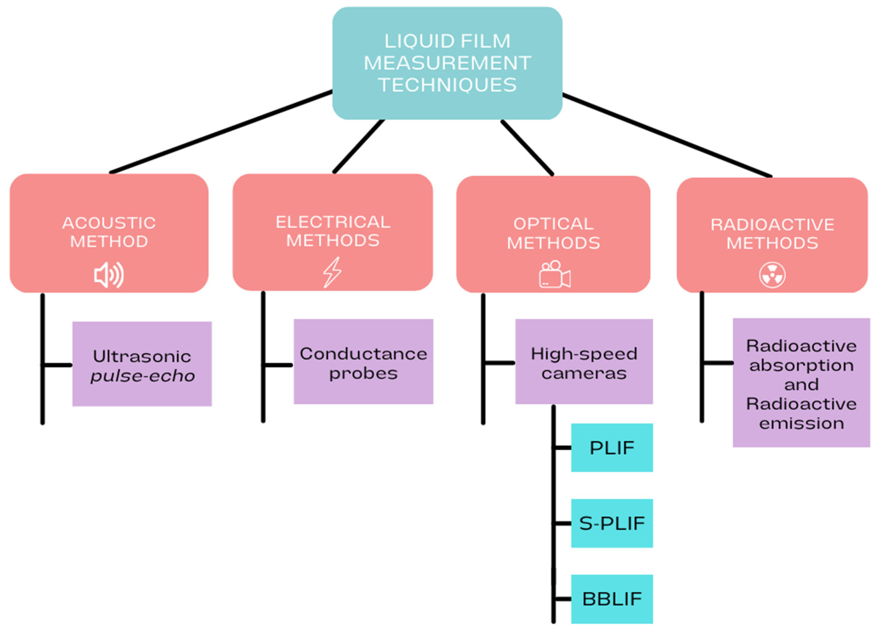
1. Introduction
2. Experimental Apparatus
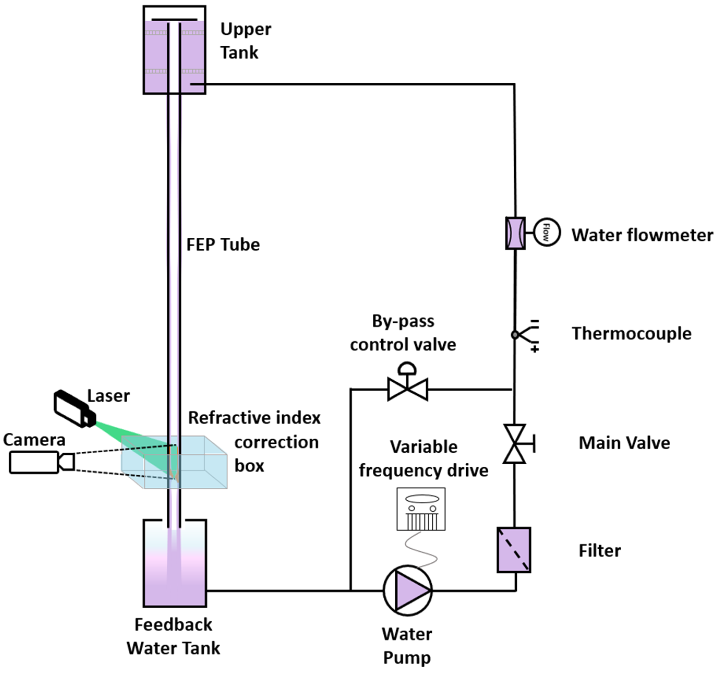
2.1. Instrumentation Used in the CAPELON Facility
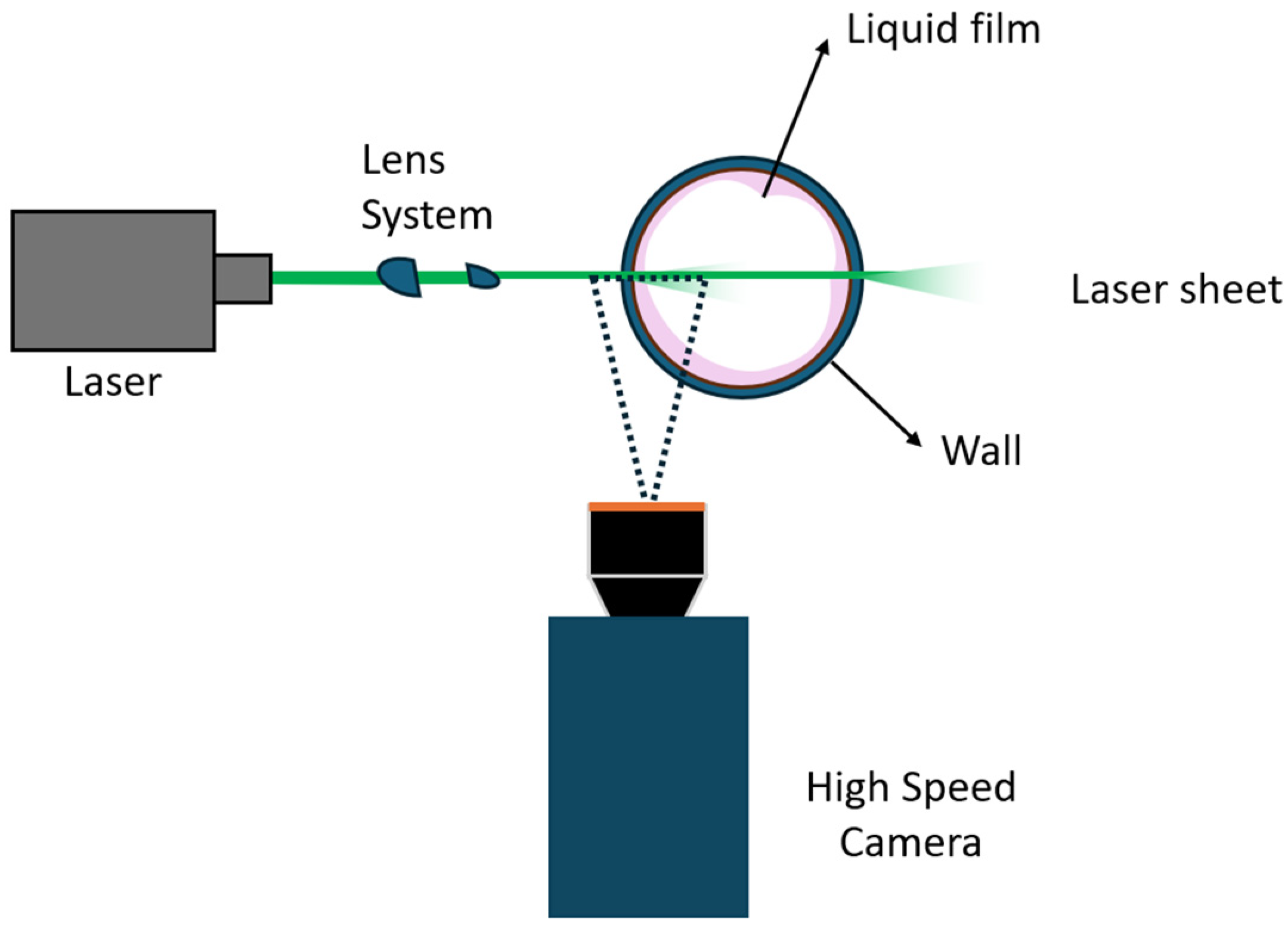
2.2. PLIF Setup
3. Implementation and Analysis of PLIF Experimental Techniques
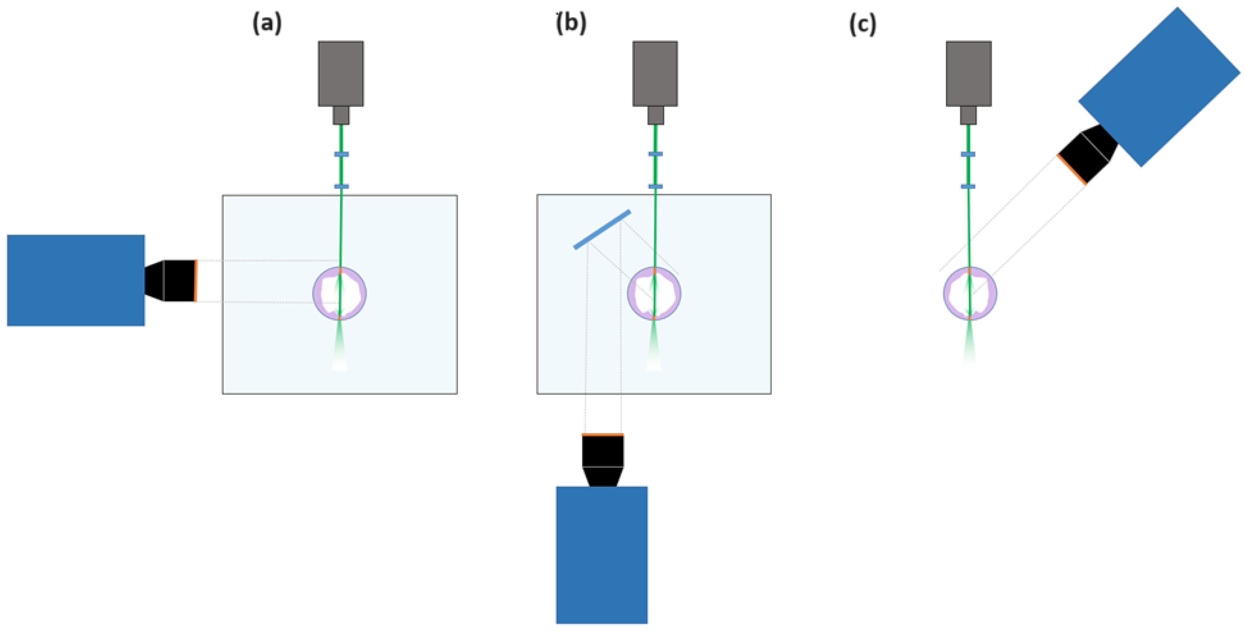
3.1. Configurations PLIF RIM90, PLIF RIM40, and PLIF nRIM40
3.2. Image Post-Processing
- Initially, Tagged Image File Format (TIFF) images are imported into MATLAB® in grayscale.
- The wall is detected during the calibration, but a first check is done to ensure that the camera has not been moved, considering that even small vibrations can cause a change of position of a few pixels. In addition, an algorithm evaluates its verticality.
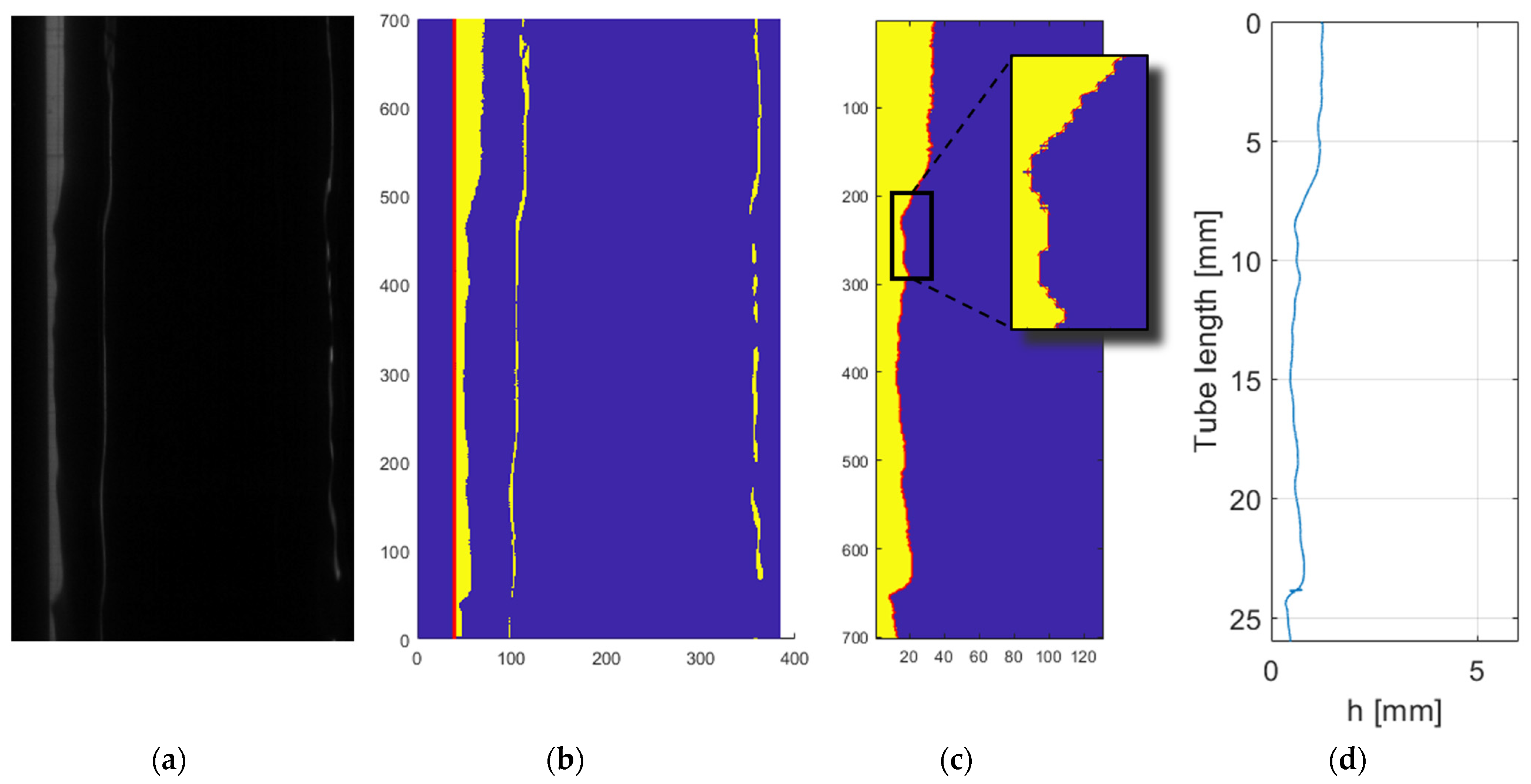
- Subsequently, a binarization process starts based on the image brightness.
- The next step entails the removal of unnecessary portions of each snapshot to reduce the computational time required for image processing.
- Employing the binarized image, the subpixel algorithm detects the location of the interface. This process employs Sobel filtering with 3 × 3 convolutional kernels. For a deeper understanding of this process, refer to [20].
- Following interface detection, the film thickness is determined by applying the relationship between pixels and millimeters obtained from a calibration image at the onset of the runs.
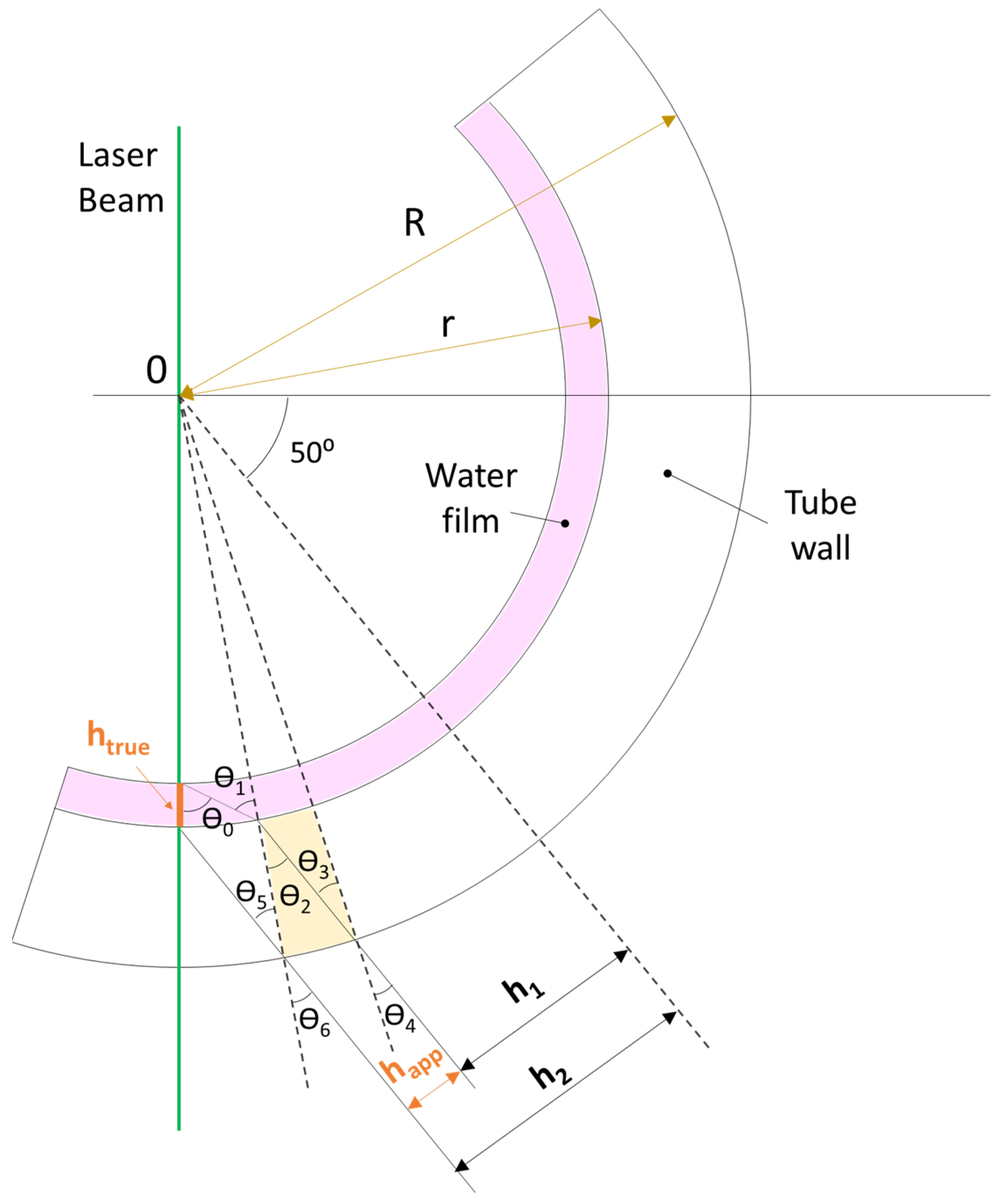
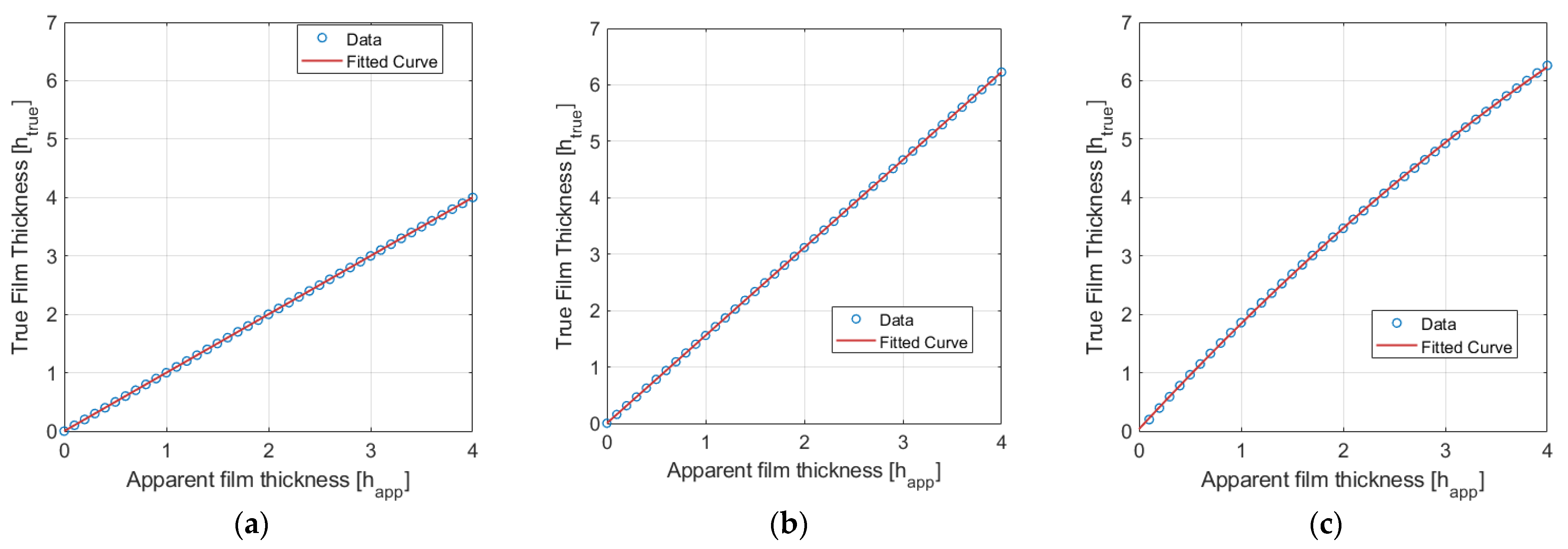
- Subsequently, the apparent film thickness undergoes correction to calculate the true film thickness (Equations (5) and (6)).
- A moving mean filter is then applied, employing a window of 16 pixels to mitigate noise, particularly that arising from droplet detachment and deposition.
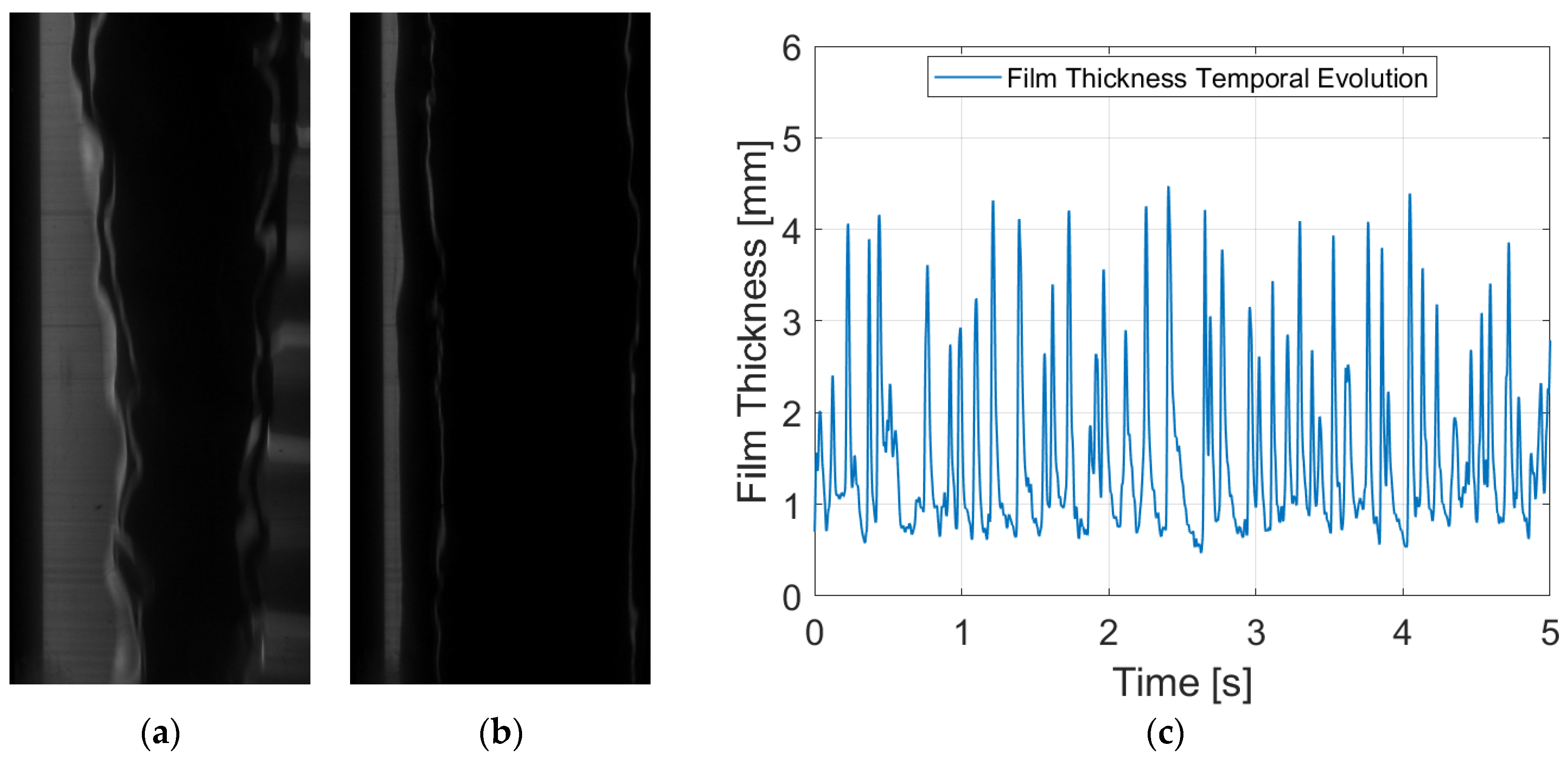
- Lastly, the composition of the film over time is computed by processing all the snapshots.
3.3. Error Estimation
4. Results and Discussion
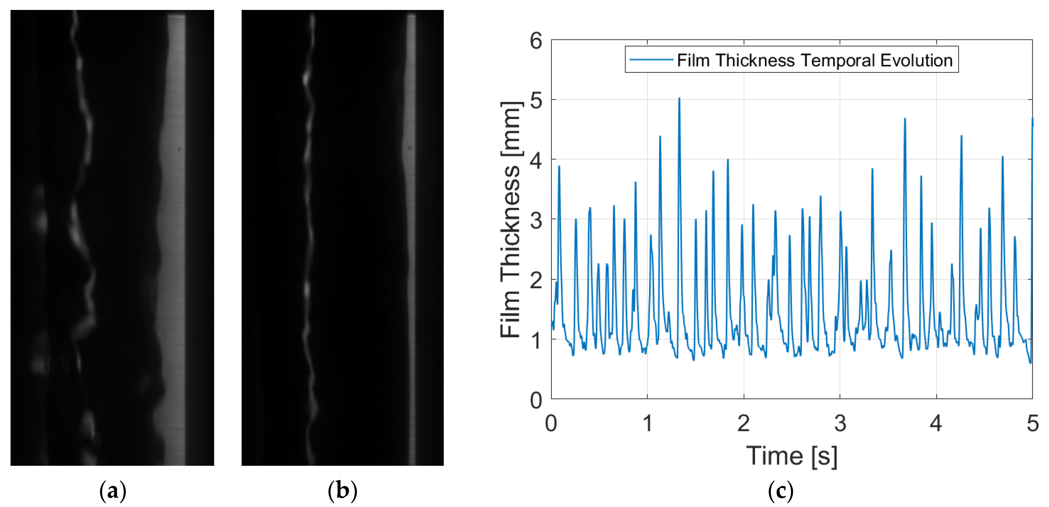
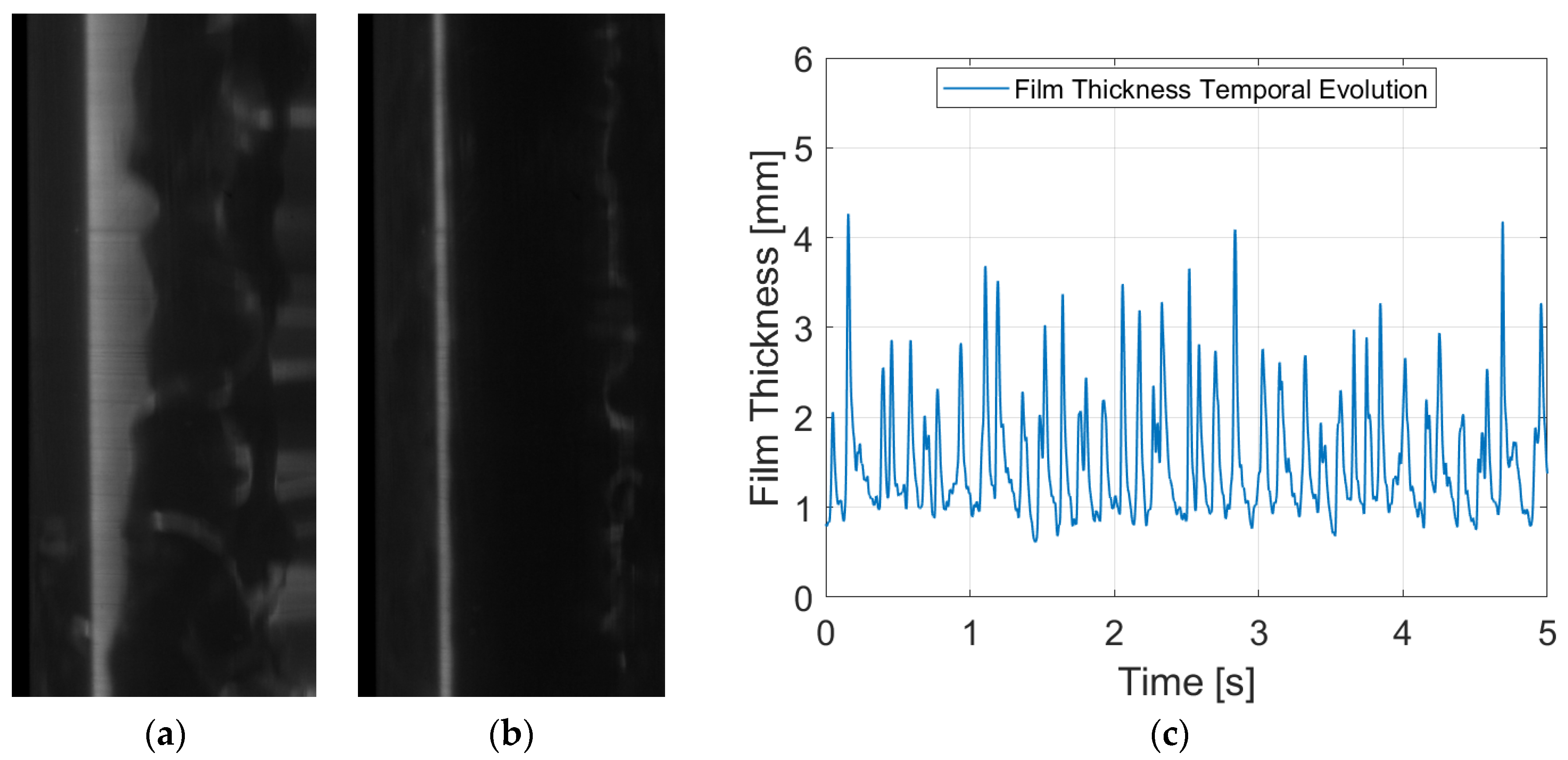
4.1. Results for the Temporal Evolution of the Liquid Film Thickness
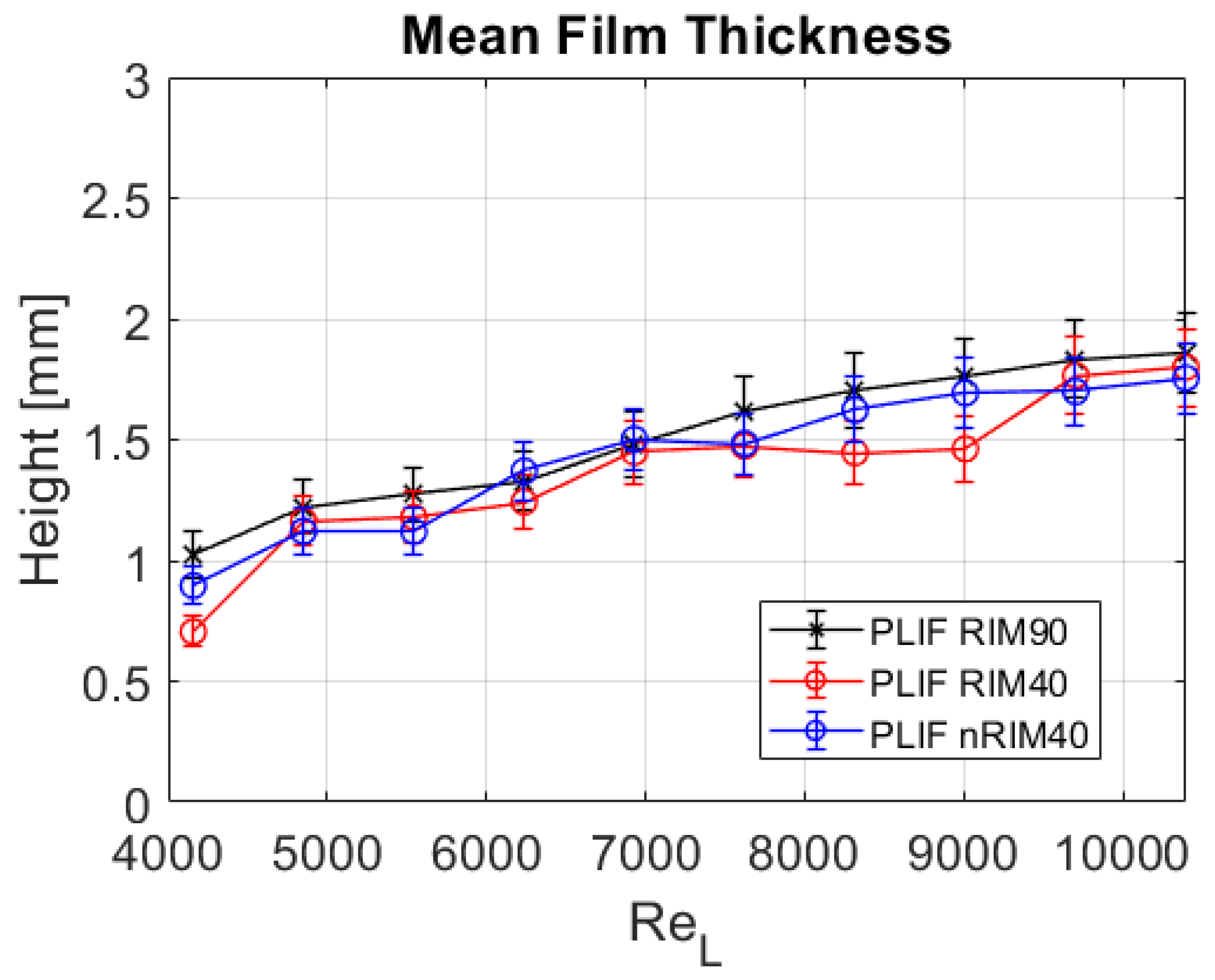
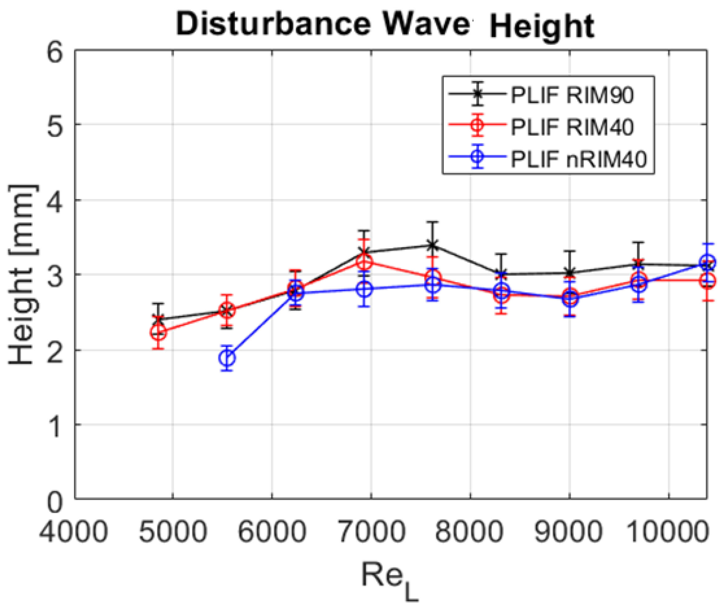
4.2. Results for the Figures of Merit of the Liquid Film
5. Conclusions
Author Contributions
Funding
Institutional Review Board Statement
Informed Consent Statement
Data Availability Statement
Acknowledgments
Conflicts of Interest
Nomenclature
| Acronyms | |
| A-PLIF | Acute Planar Laser-Induced Fluorescence |
| BBLIF | Brightness-Based Laser-Induced Fluorescence |
| BWR | Boiling Water Reactor |
| CAPELON | Facility Acronym of Caracterización de Película Ondulatoria |
| CMOS | Complementary metal–oxide–semiconductor |
| DW | Disturbance Waves |
| FEP | Fluorinated Propylene Ethylene |
| LIF | Laser-Induced Fluorescence |
| N-PLIF | Normal Planar Laser-Induced Fluorescence |
| nRIM | Non-Refractive Index Matching |
| PFA | Perfluoroalkoxy alkanes |
| PLIF | Planar Laser-Induced Fluorescence |
| PLIF40 | Planar Laser-Induced Fluorescence at 40° angle |
| PTFE | Polytetrafluoroethylene |
| RIM | Refractive Index Matching |
| ROI | Region of Interest |
| FoM | Figure of Merit |
| RW | Ripple Waves |
| SMR | Small Modular Reactor |
| TIFF | Tagged Image File Format |
| Variables | |
| Reynolds number | |
| Significance level | |
| Film thickness | |
| Apparent film thickness measured by the high-speed camera | |
| True film thickness | |
| Mean film thickness | |
| Disturbance wave height from the wall | |
| Disturbance wave frequency | |
| Refractive index of water | |
| Refractive index of the tube | |
| Refractive index of the air | |
| Superficial velocity of the liquid | |
| Angles of light refraction | |
References
- Cuadros, J.; Rivera, Y.; Berna, C.; Escrivá, A.; Muñoz-Cobo, J.; Monrós-Andreu, G.; Chiva, S. Characterization of the gas-liquid interfacial waves in vertical upward co-current annular flows. Nucl. Eng. Des. 2019, 346, 112–130. [Google Scholar] [CrossRef]
- Zhao, Y.; Markides, C.N.; Matar, O.K.; Hewitt, G.F. Disturbance wave development in two-phase gas–liquid upwards vertical annular flow. Int. J. Multiph. Flow 2013, 55, 111–129. [Google Scholar] [CrossRef]
- Ju, P.; Liu, Y.; Ishii, M.; Hibiki, T. Prediction of rod film thickness of vertical upward co-current adiabatic flow in rod bundle. Ann. Nucl. Energy 2018, 121, 1–10. [Google Scholar] [CrossRef]
- Lin, R.; Wang, K.; Liu, L.; Zhang, Y.; Dong, S. Study on the characteristics of interfacial waves in annular flow by image analysis. Chem. Eng. Sci. 2020, 212, 115336. [Google Scholar] [CrossRef]
- Berna, C.; Escrivá, A.; Muñoz-Cobo, J.; Herranz, L. Review of droplet entrainment in annular flow: Interfacial waves and onset of entrainment. Prog. Nucl. Energy 2014, 74, 14–43. [Google Scholar] [CrossRef]
- Berna, C.; Escrivá, A.; Muñoz-Cobo, J.; Herranz, L. Review of droplet entrainment in annular flow: Characterization of the entrained droplets. Prog. Nucl. Energy 2015, 79, 64–86. [Google Scholar] [CrossRef]
- Belt, R.J.; Van’t Westende, J.M.C.; Prasser, H.M.; Portela, L.M. Time spatially resolved measurements of interfacial waves in vertical annular flow. Int. J. Multiph. Flow 2010, 36, 570–587. [Google Scholar] [CrossRef]
- Cherdantsev, A.; An, J.; Charogiannis, A.; Markides, C. Simultaneous application of two laser-induced fluorescence approaches for film thickness measurements in annular gas-liquid flows. Int. J. Multiph. Flow 2019, 119, 237–258. [Google Scholar] [CrossRef]
- Sawant, P.; Ishii, M.; Hazuku, T.; Takamasa, T.; Mori, M. Properties of disturbance waves in vertical annular two-phase flow. Nucl. Eng. Des. 2008, 238, 3528–3541. [Google Scholar] [CrossRef]
- Setyawan, A.; Indarto, I.; Deendarlianto, D. Measurement of liquid holdup by using conductance probe sensor in horizontal annular flow. J. Adv. Res. Fluid Mech. Therm. Sci. 2019, 53, 11–24. [Google Scholar]
- Xue, T.; Zhang, T.; Li, Z. A Method to Suppress the Effect of Total Reflection on PLIF Imaging in Annular Flow. IEEE Trans. Instrum. Meas. 2022, 71, 3167775. [Google Scholar] [CrossRef]
- Xue, T.; Zhang, S.; Wu, B. Study of spatiotemporally resolved temperature field and heat transfer in liquid film using PLIF. Heat Mass Transf. 2019, 55, 845–854. [Google Scholar] [CrossRef]
- Xue, T.; Li, H.; Zhang, T. Imaging and Investigation with Innovative PLIF40 for Improved Film Thickness Measurements in Annular Flow. Exp. Therm. Fluid Sci. 2024, 150, 111032. [Google Scholar] [CrossRef]
- Rivera, Y.; Berna, C.; Muñoz-Cobo, J.; Escrivá, A.; Córdova, Y. Experiments in free falling and downward cocurrent annular flows—Characterization of liquid films and interfacial waves. Nucl. Eng. Des. 2022, 392, 111769. [Google Scholar] [CrossRef]
- Chu, K.J.; Dukler, A.E. Statistical characteristics of thin, wavy films. Part II: Studies on the substrate and its wave structure. Am. Inst. Chem. Eng. J. 1974, 20, 695–706. [Google Scholar] [CrossRef]
- Chu, K.J.; Dukler, A.E. Statistical characteristics of thin, wavy films. Part III: Structure of the large waves and their resistances to gas flow. Am. Inst. Chem. Eng. J. 1975, 20, 695–706. [Google Scholar] [CrossRef]
- Ju, P.; Yang, X.; Schlegel, J.P.; Liu, Y.; Hibiki, T.; Ishii, M. Average liquid film thickness of annular air-water two-phase flow in 8 × 8 rod bundle. Int. J. Heat Fluid Flow 2018, 73, 63–73. [Google Scholar] [CrossRef]
- Skjæraasen, O.; Kesana, N.R. X-ray measurements of thin liquid films in gas–liquid pipe flow. Int. J. Multiph. Flow 2020, 131, 103391. [Google Scholar] [CrossRef]
- Wang, M.; Zheng, D.; Xu, Y. A new method for liquid film thickness measurement based on ultrasonic echo resonance technique in gas-liquid flow. Measurement 2019, 146, 447–457. [Google Scholar] [CrossRef]
- Rivera, Y.; Bidon, M.; Muñoz-Cobo, J.-L.; Berna, C.; Escrivá, A. A Comparative Analysis of Conductance Probes and High-Speed Camera Measurements for Interfacial Behavior in Annular Air–Water Flow. Sensors 2023, 23, 8617. [Google Scholar] [CrossRef]
- Schubring, D.; Shedd, T.; Hurlburt, E. Studying disturbance waves in vertical annular flow with high-speed video. Int. J. Multiph. Flow 2010, 36, 385–396. [Google Scholar] [CrossRef]
- Alekseenko, S.V.; Cherdantsev, A.V.; Heinz, O.M.; Kharlamov, S.M.; Markovich, D.M. Analysis of spatial and temporal evolution of disturbance waves and ripples in annular gas–liquid flow. Int. J. Multiph. Flow 2014, 67, 122–134. [Google Scholar] [CrossRef]
- Alekseenko, S.V.; Antipin, V.A.; Cherdantsev, A.V.; Kharlamov, S.M.; Markovich, D.M. Investigation of Waves Interaction in Annular Gas–Liquid Flow Using High-Speed Fluorescent Visualization Technique. Microgravity Sci. Technol. 2008, 20, 271–275. [Google Scholar] [CrossRef]
- Alekseenko, S.; Cherdantsev, A.; Cherdantsev, M.; Isaenkov, S.; Kharlamov, S.; Markovich, D. Application of a high-speed laser-induced fluorescence technique for studying the three-dimensional structure of annular gas–liquid flow. Exp. Fluids 2012, 53, 77–89. [Google Scholar] [CrossRef]
- Schubring, D.; Ashwood, A.; Shedd, T.; Hurlburt, E. Planar laser-induced fluorescence (PLIF) measurements of liquid film thickness in annular flow. Part I: Methods and data. Int. J. Multiph. Flow 2010, 36, 815–824. [Google Scholar] [CrossRef]
- Charogiannis, A.; An, J.S.; Voulgaropoulos, V.; Markides, C.N. Structured planar laser-induced fluorescence (S-PLIF) for the accurate identification of interfaces in multiphase flows. Int. J. Multiph. Flow 2019, 118, 193–204. [Google Scholar] [CrossRef]
- Cherdantsev, A.; Bobylev, A.; Guzanov, V.; Kvon, A.; Kharlamov, S. Measuring liquid film thickness based on the brightness level of the fluorescence: Methodical overview. Int. J. Multiph. Flow 2023, 168. [Google Scholar] [CrossRef]
- Li, T.; Lian, T.; Huang, B.; Yang, X.; Liu, X.; Li, Y. Liquid film thickness measurements on a plate based on brightness curve analysis with acute PLIF method. Int. J. Multiph. Flow 2021, 136, 103549. [Google Scholar] [CrossRef]
- Helmers, T.; Kemper, P.; Mießner, U.; Thöming, J. Refractive index matching (RIM) using double-binary liquid–liquid mixtures. Exp. Fluids 2020, 61, 64. [Google Scholar] [CrossRef]
- Danielsson, P.E.; Seger, O. Generalized and Separable Sobel Operators. In Machine Vision for Three-Dimensional Scenes; Freeman, H., Ed.; Academic Press: Cambridge, MA, USA, 1990. [Google Scholar]
- Patnaik, S.; Yang, Y.M. Soft Computing Techniques in Vision Science 395; Springer: Berlin/Heidelberg, Germany, 2012. [Google Scholar]


| Water Flow, | Reynolds Number, | Superficial Velocity, |
|---|---|---|
| 3.0 | 4200 | 0.25 |
| 3.5 | 4900 | 0.29 |
| 4.0 | 5500 | 0.33 |
| 4.5 | 6200 | 0.37 |
| 5.0 | 7000 | 0.41 |
| 5.5 | 7600 | 0.46 |
| 6.0 | 8300 | 0.50 |
| 6.5 | 9000 | 0.54 |
| 7.0 | 9700 | 0.58 |
| 7.5 | 10,400 | 0.62 |
| Figure of Merit | ||||||
|---|---|---|---|---|---|---|
| Mean | Max | Mean | Max | Mean | Max | |
| 1.5 | 1.6 | 7.5 | 7.8 | 7.6 | 8.0 | |
| 5.1 | 5.8 | 6.0 | 7.6 | 7.9 | 9.6 | |
| 6.0 | 7.3 | 0.0 | 0.0 | 6.0 | 7.3 | |
Disclaimer/Publisher’s Note: The statements, opinions and data contained in all publications are solely those of the individual author(s) and contributor(s) and not of MDPI and/or the editor(s). MDPI and/or the editor(s) disclaim responsibility for any injury to people or property resulting from any ideas, methods, instructions or products referred to in the content. |
© 2024 by the authors. Licensee MDPI, Basel, Switzerland. This article is an open access article distributed under the terms and conditions of the Creative Commons Attribution (CC BY) license (https://creativecommons.org/licenses/by/4.0/).
Share and Cite
Rivera, Y.; Bascou, D.; Blanco, D.; Álvarez-Piñeiro, L.; Berna, C.; Muñoz-Cobo, J.-L.; Escrivá, A. Comparison of Refractive Index Matching Techniques and PLIF40 Measurements in Annular Flow. Sensors 2024, 24, 2317. https://doi.org/10.3390/s24072317
Rivera Y, Bascou D, Blanco D, Álvarez-Piñeiro L, Berna C, Muñoz-Cobo J-L, Escrivá A. Comparison of Refractive Index Matching Techniques and PLIF40 Measurements in Annular Flow. Sensors. 2024; 24(7):2317. https://doi.org/10.3390/s24072317
Chicago/Turabian StyleRivera, Yago, Dorian Bascou, David Blanco, Lucas Álvarez-Piñeiro, César Berna, José-Luis Muñoz-Cobo, and Alberto Escrivá. 2024. "Comparison of Refractive Index Matching Techniques and PLIF40 Measurements in Annular Flow" Sensors 24, no. 7: 2317. https://doi.org/10.3390/s24072317
APA StyleRivera, Y., Bascou, D., Blanco, D., Álvarez-Piñeiro, L., Berna, C., Muñoz-Cobo, J.-L., & Escrivá, A. (2024). Comparison of Refractive Index Matching Techniques and PLIF40 Measurements in Annular Flow. Sensors, 24(7), 2317. https://doi.org/10.3390/s24072317