
Adaptive Extended State Observer for the Dual Active Bridge Converters


Abstract
1. Introduction
- Compared to the existing model-based method for the DAB converter, the proposed AESO method can reduce the number of current sensors, thus significantly reducing the system cost;
- The proposed AESO method effectively balances the tracking performance and disturbance suppression compared to a fixed-bandwidth ESO. Consequently, the AESO streamlines the parameter design process for the controller.
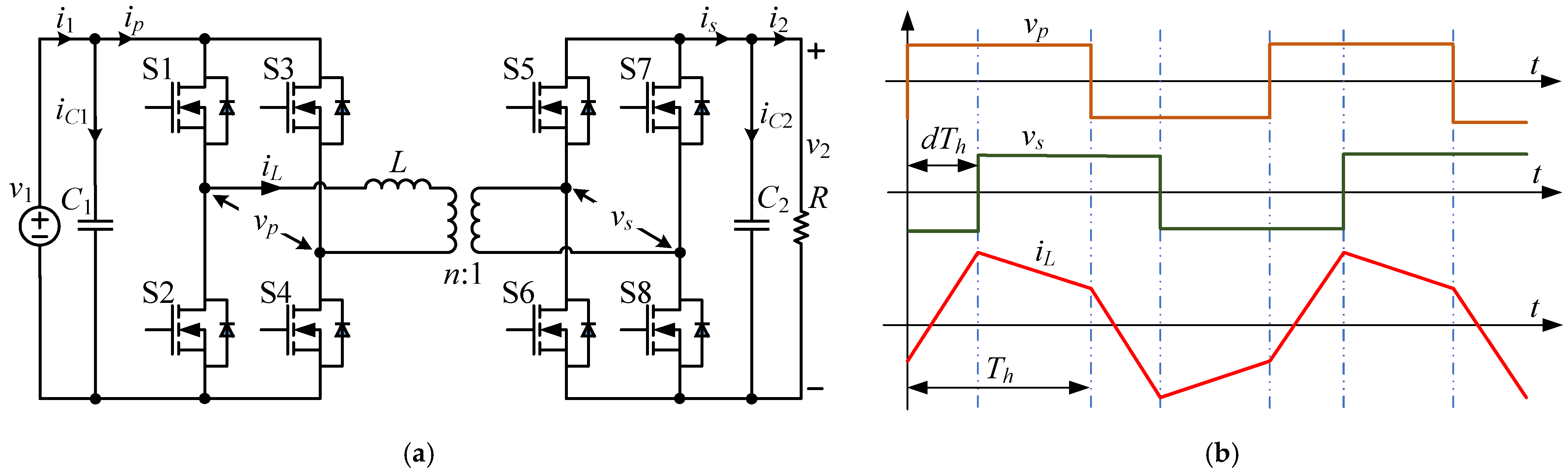
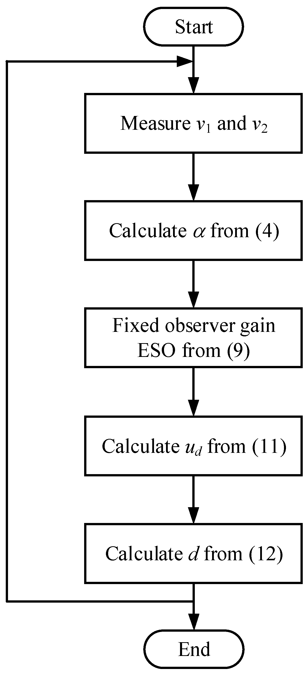
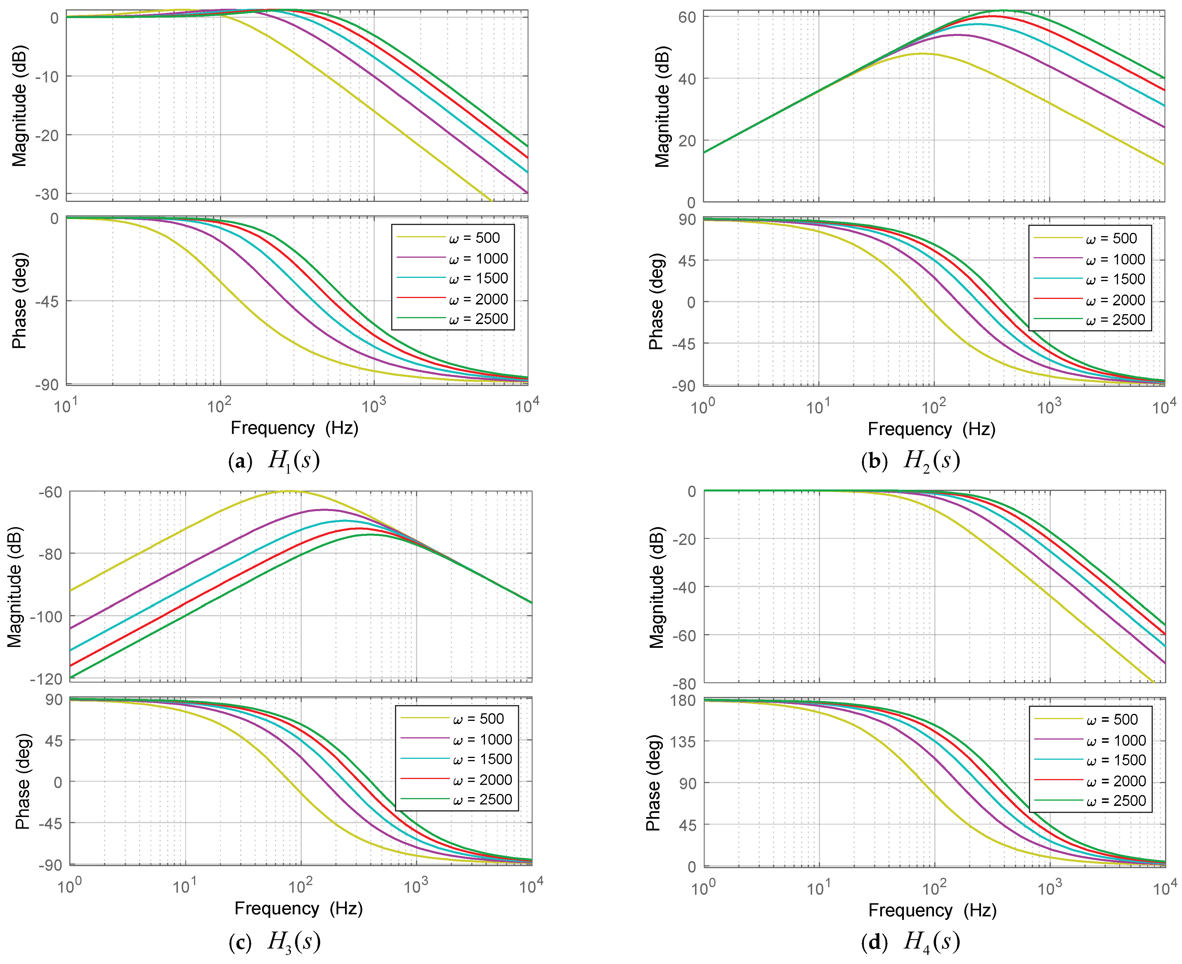
2. ESO with a Fixed Observer Bandwidth for DAB Converters
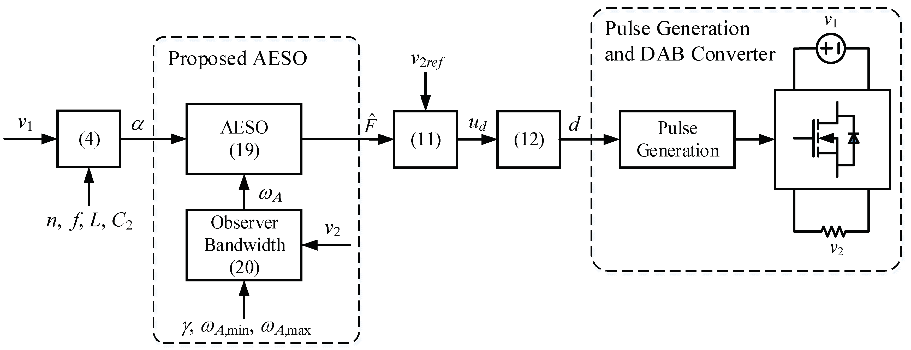
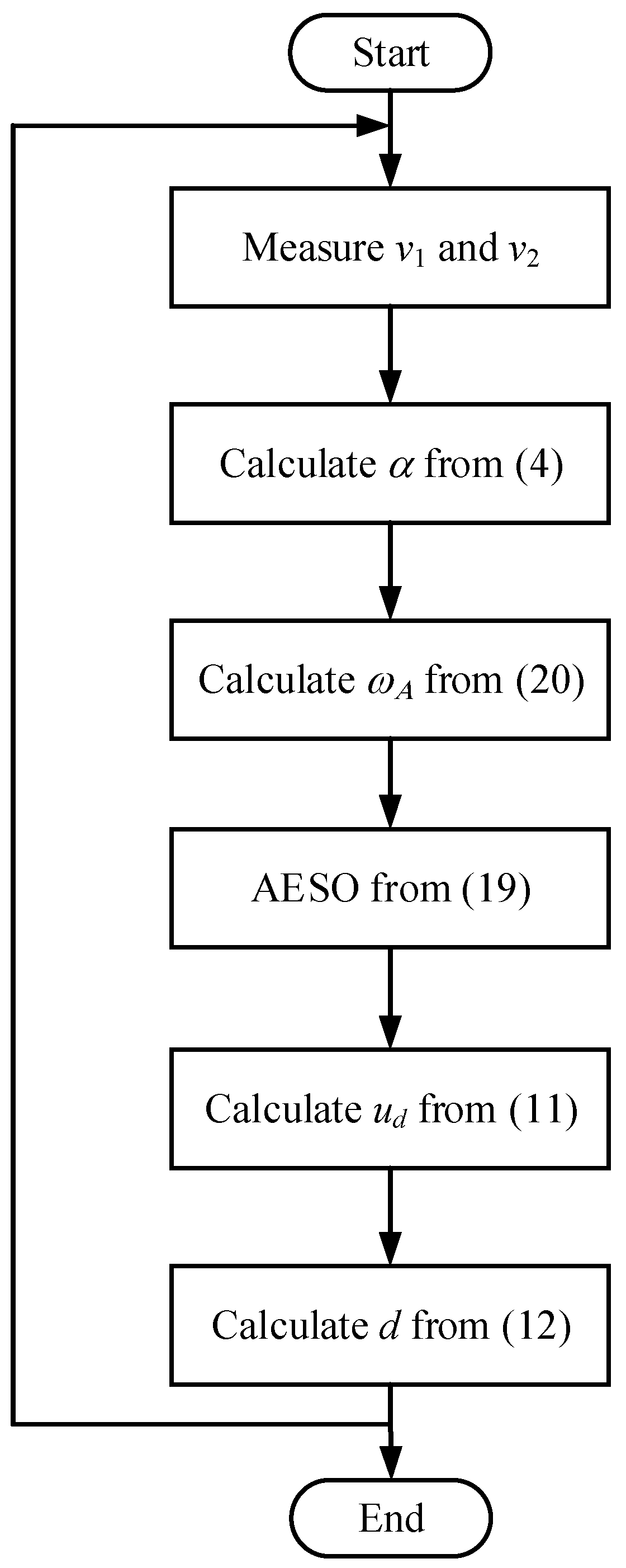
3. Proposed AESO
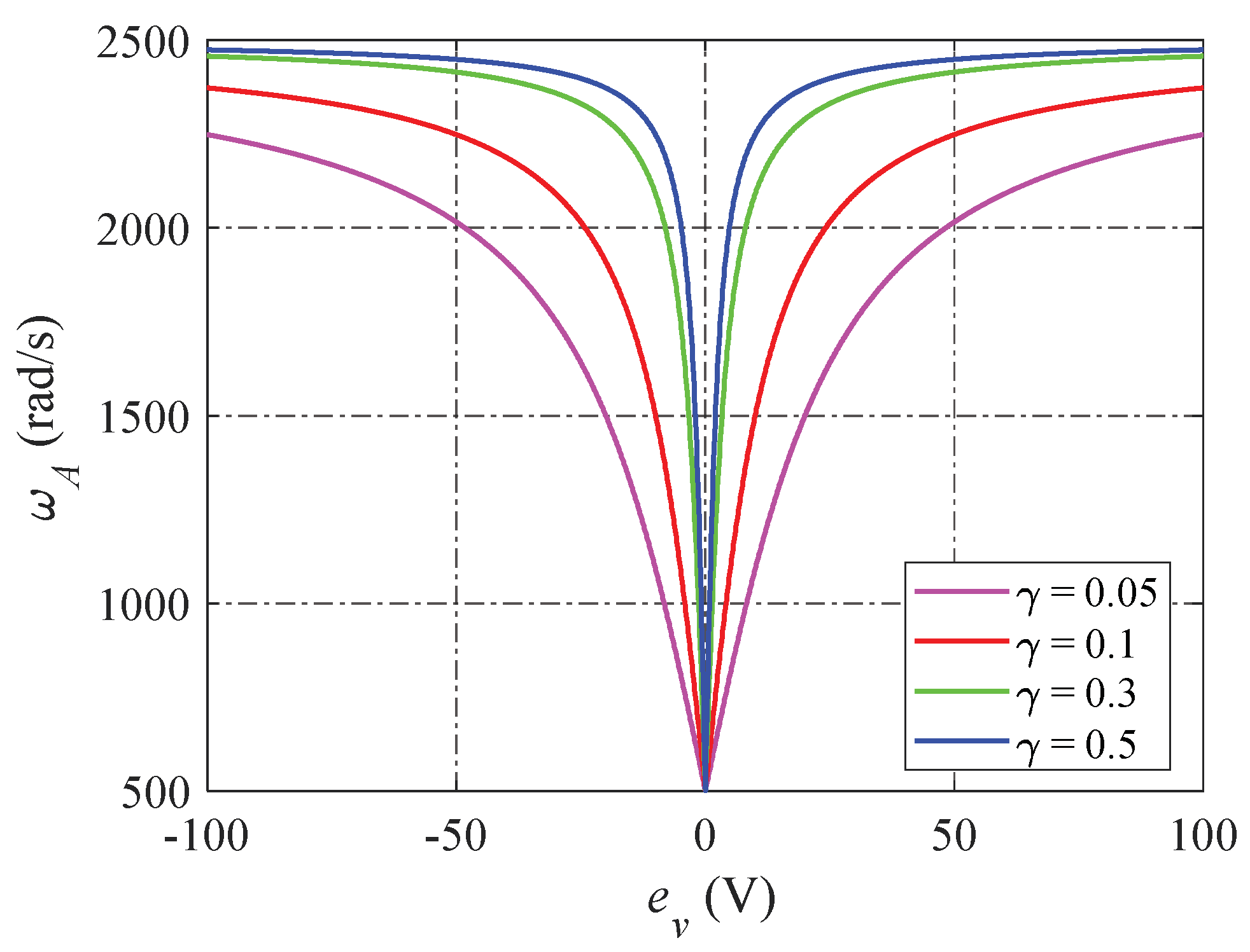
3.1. Principle of AESO
3.2. Stability Analysis
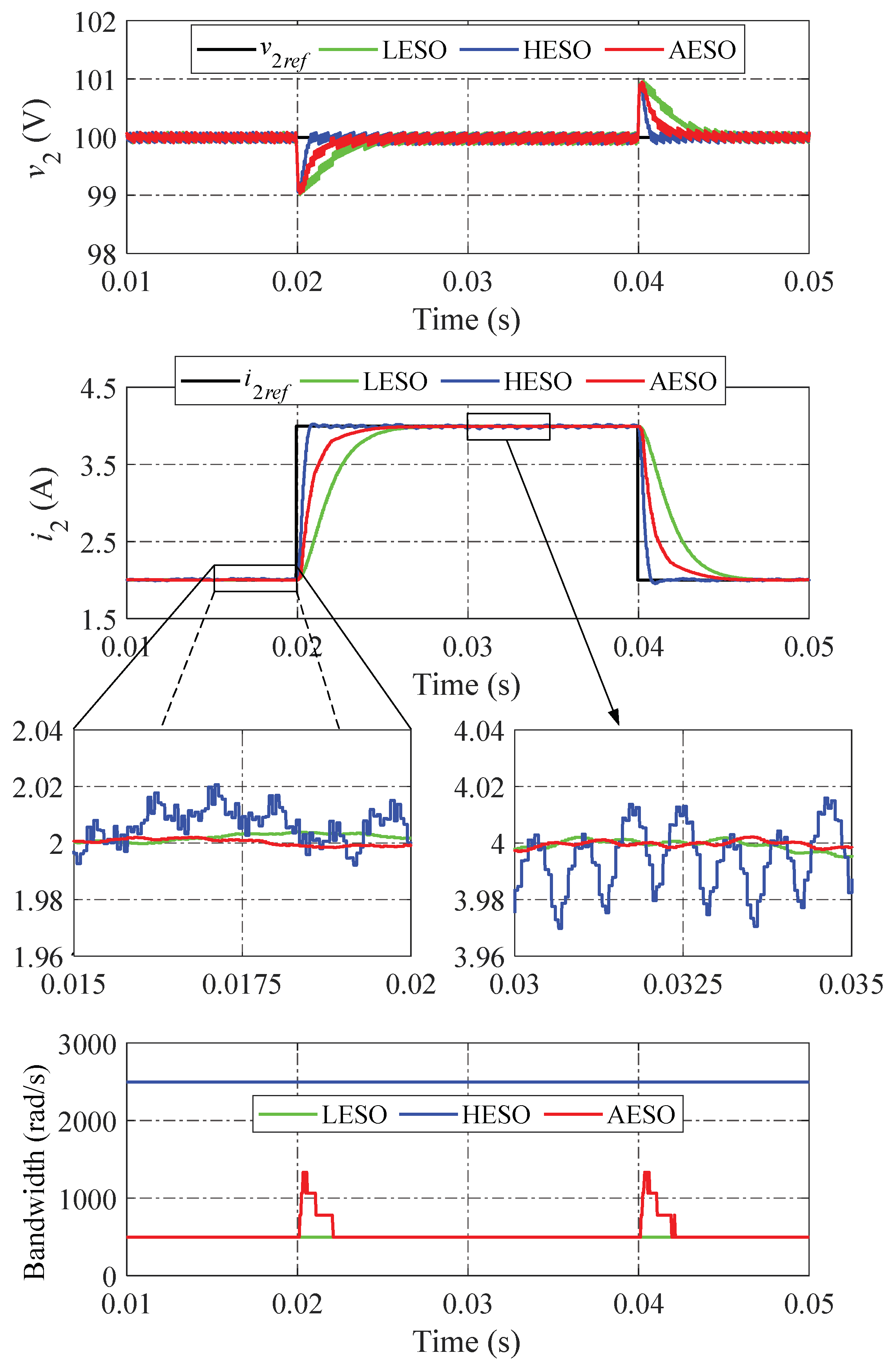
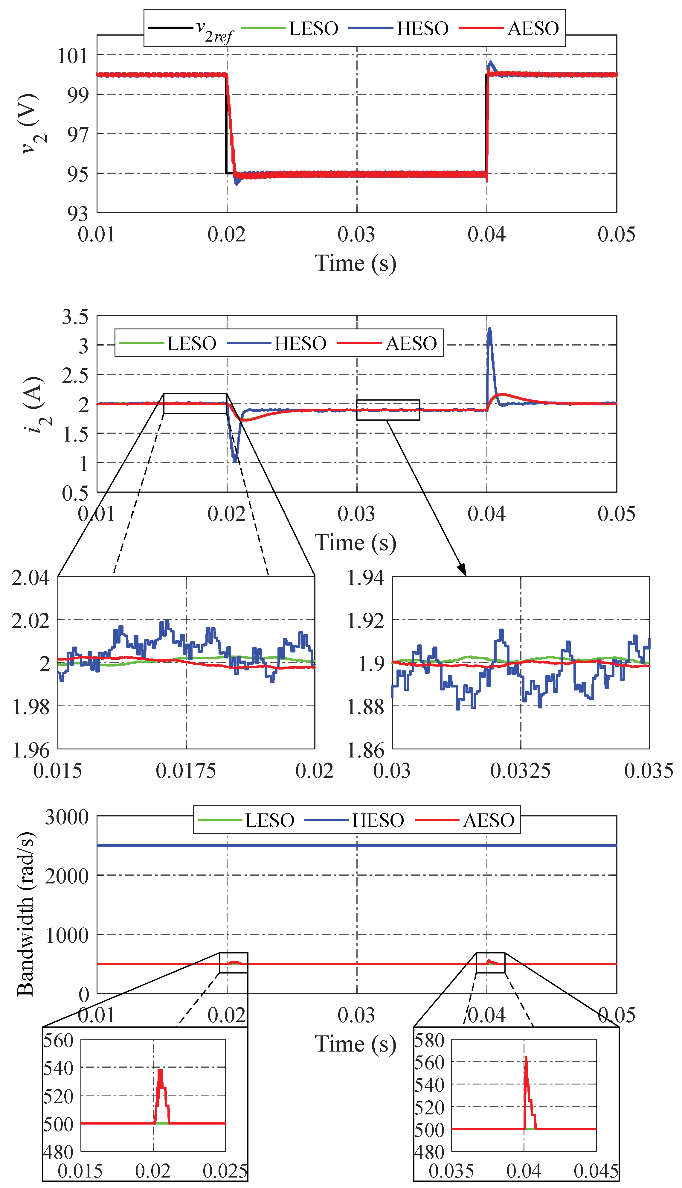
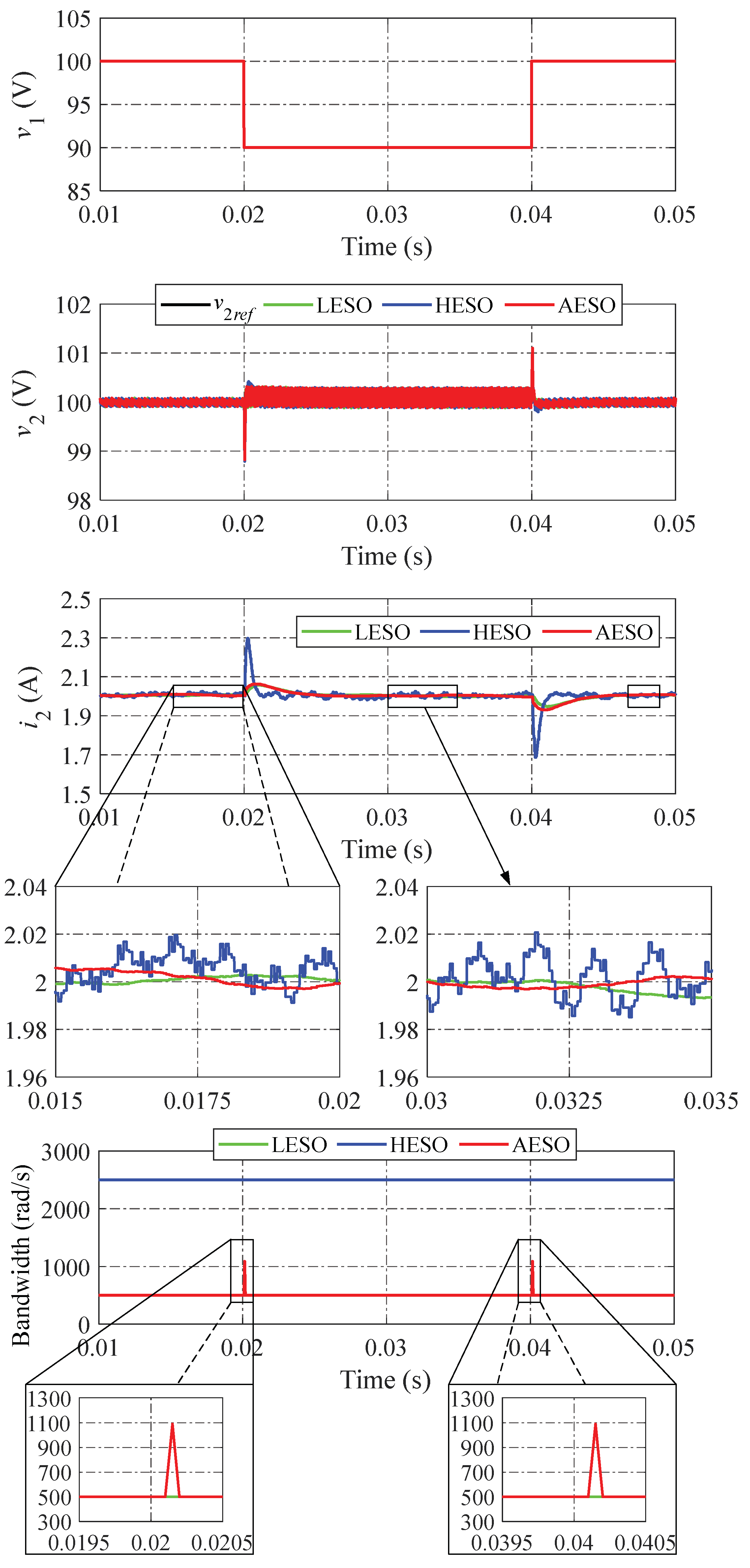
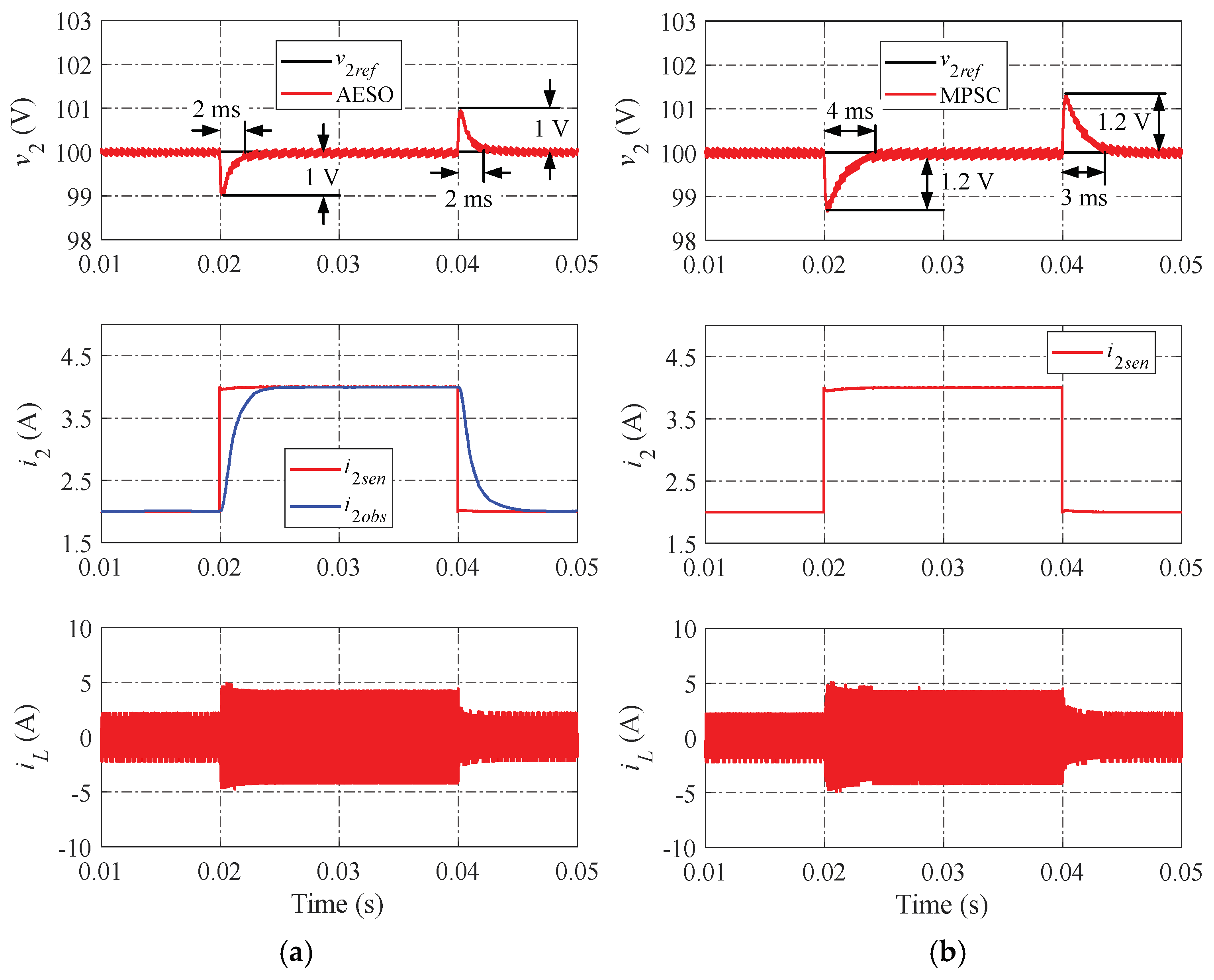
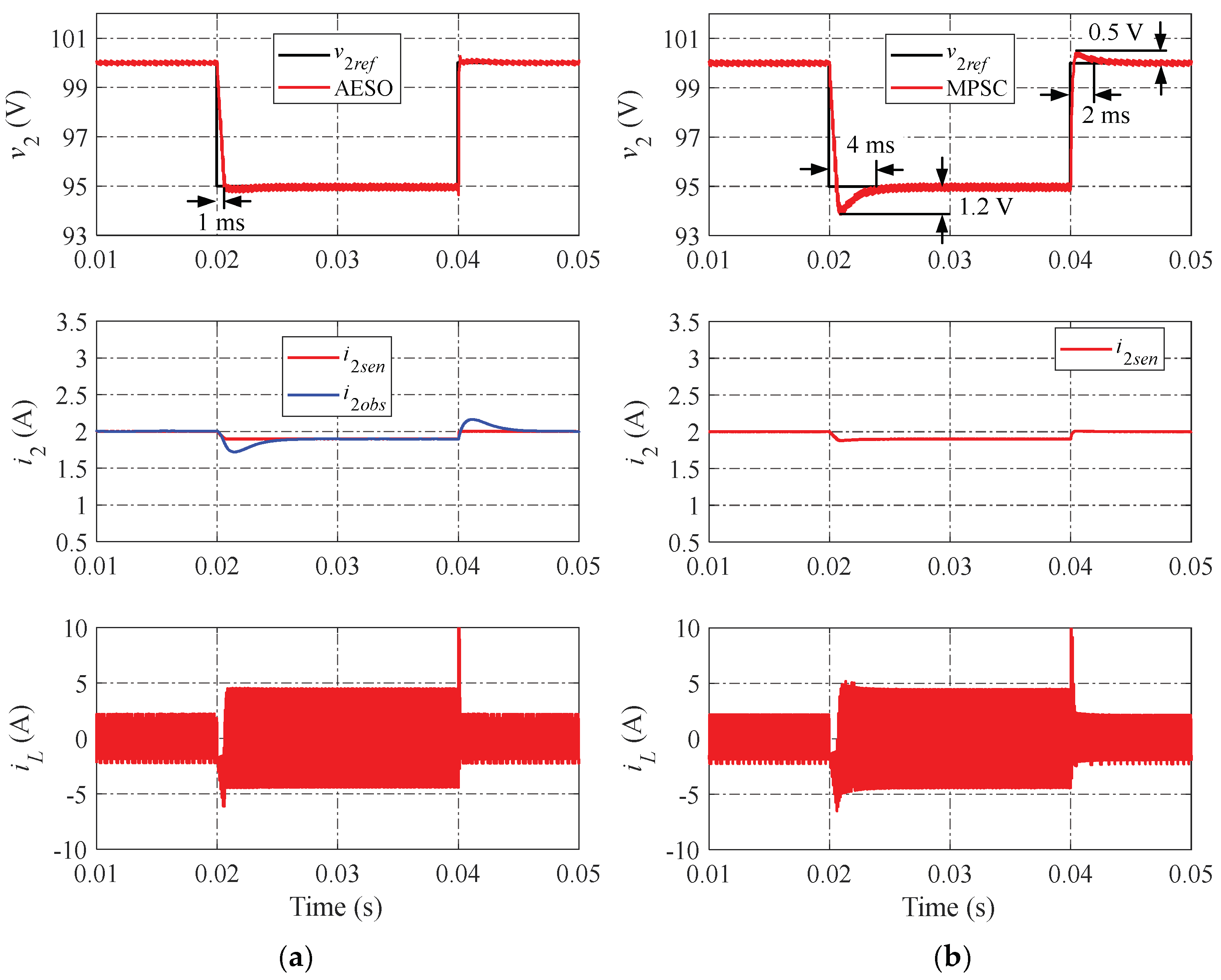
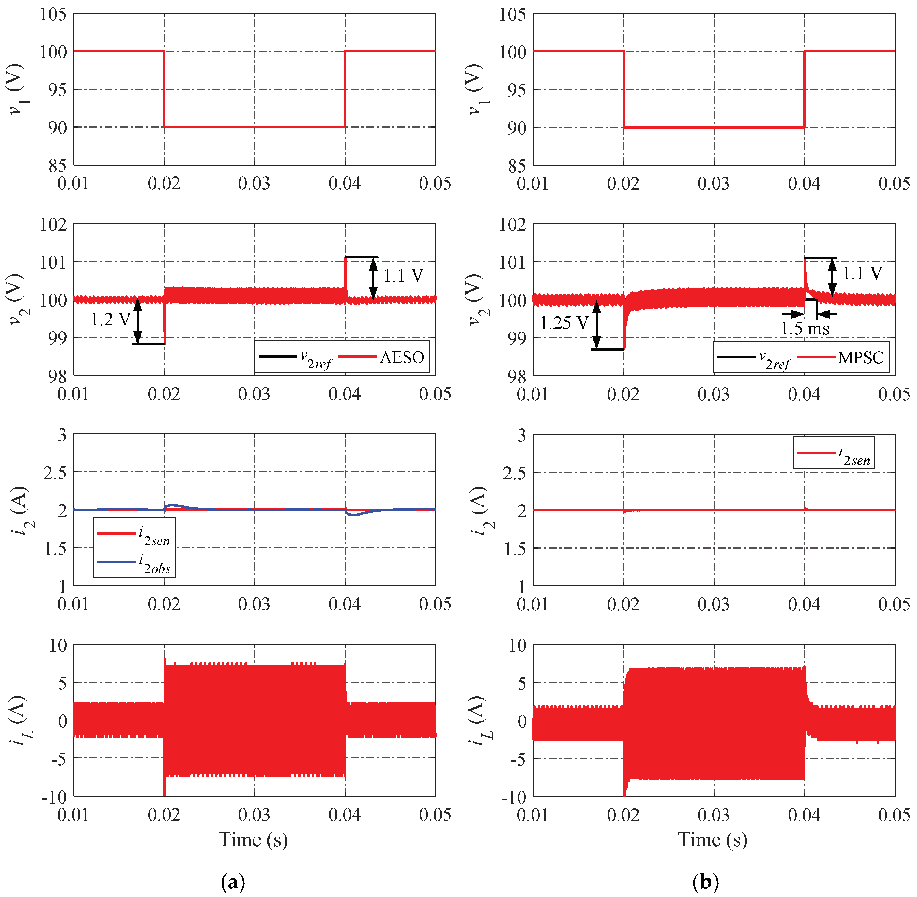
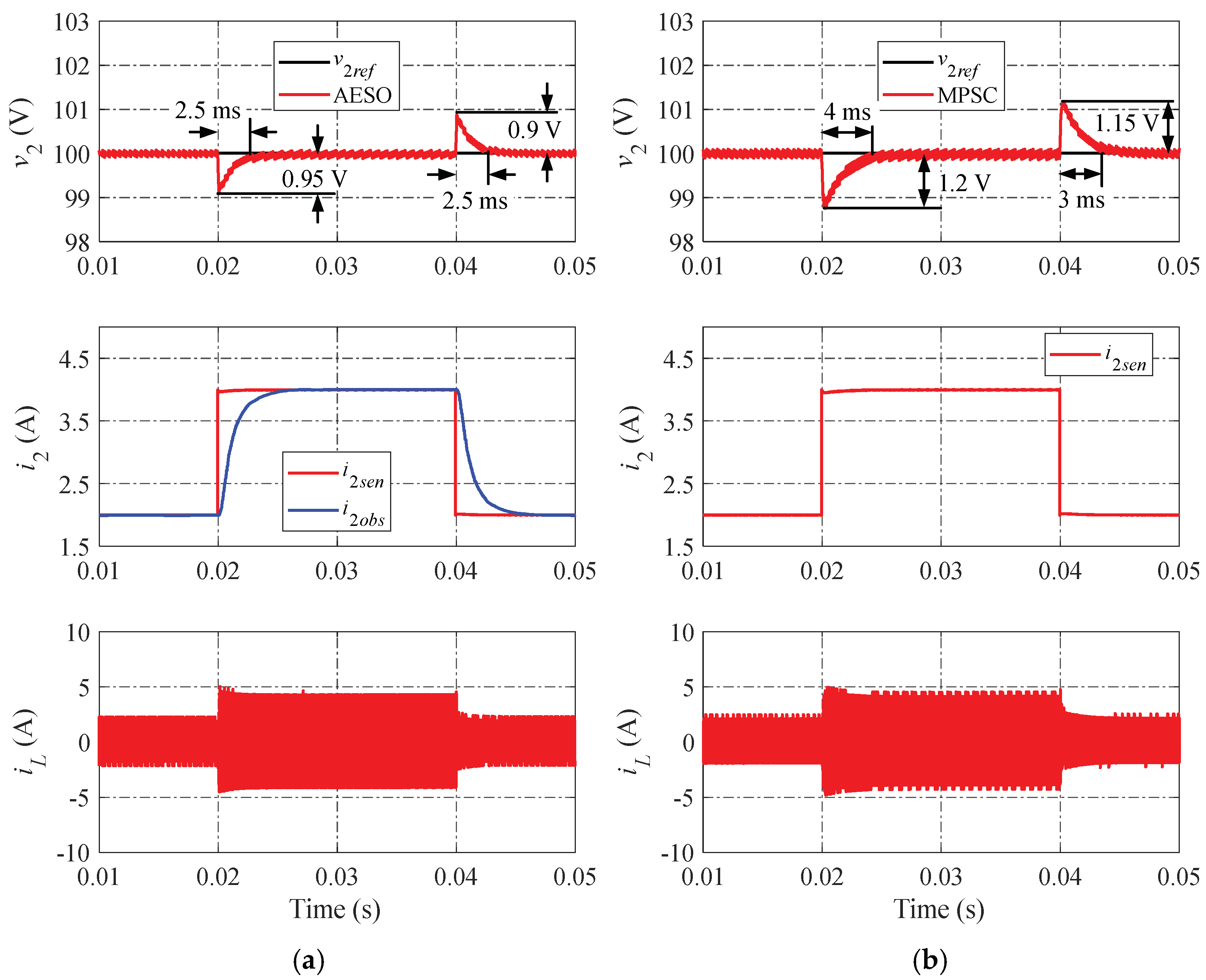
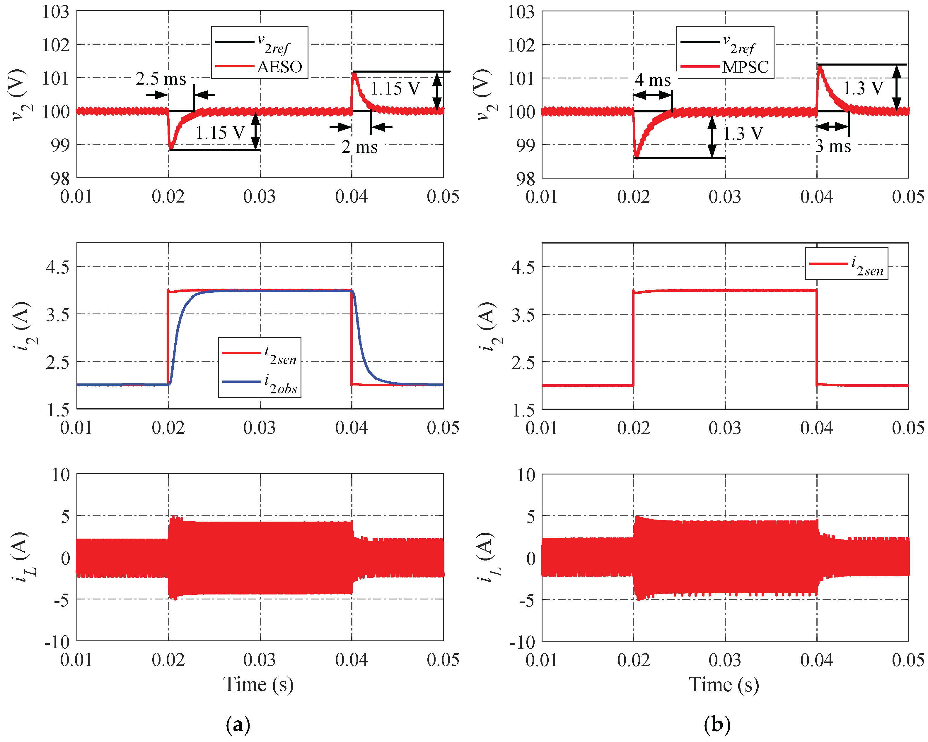
4. Simulation and Experiment Verification
4.1. Simulation
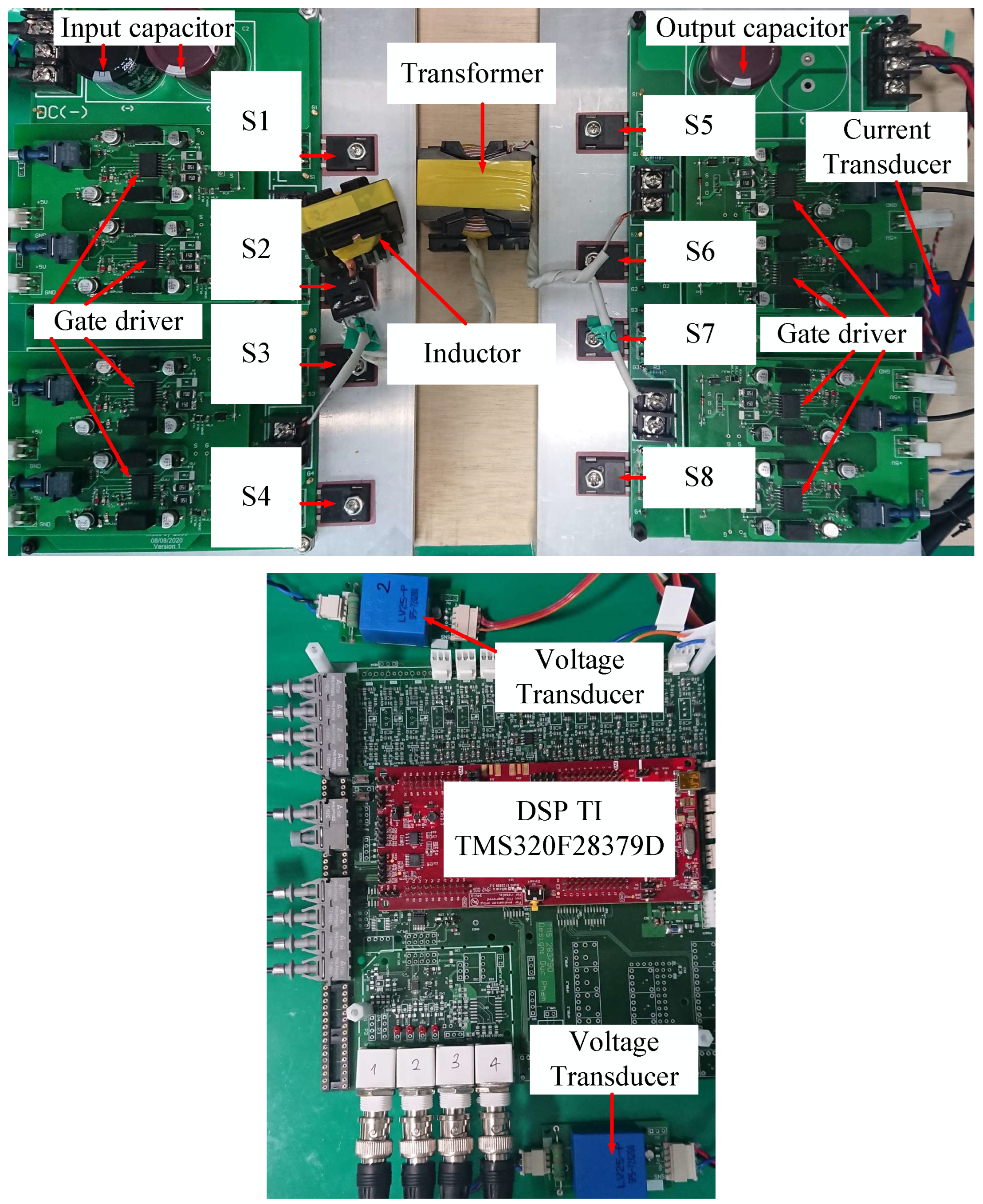
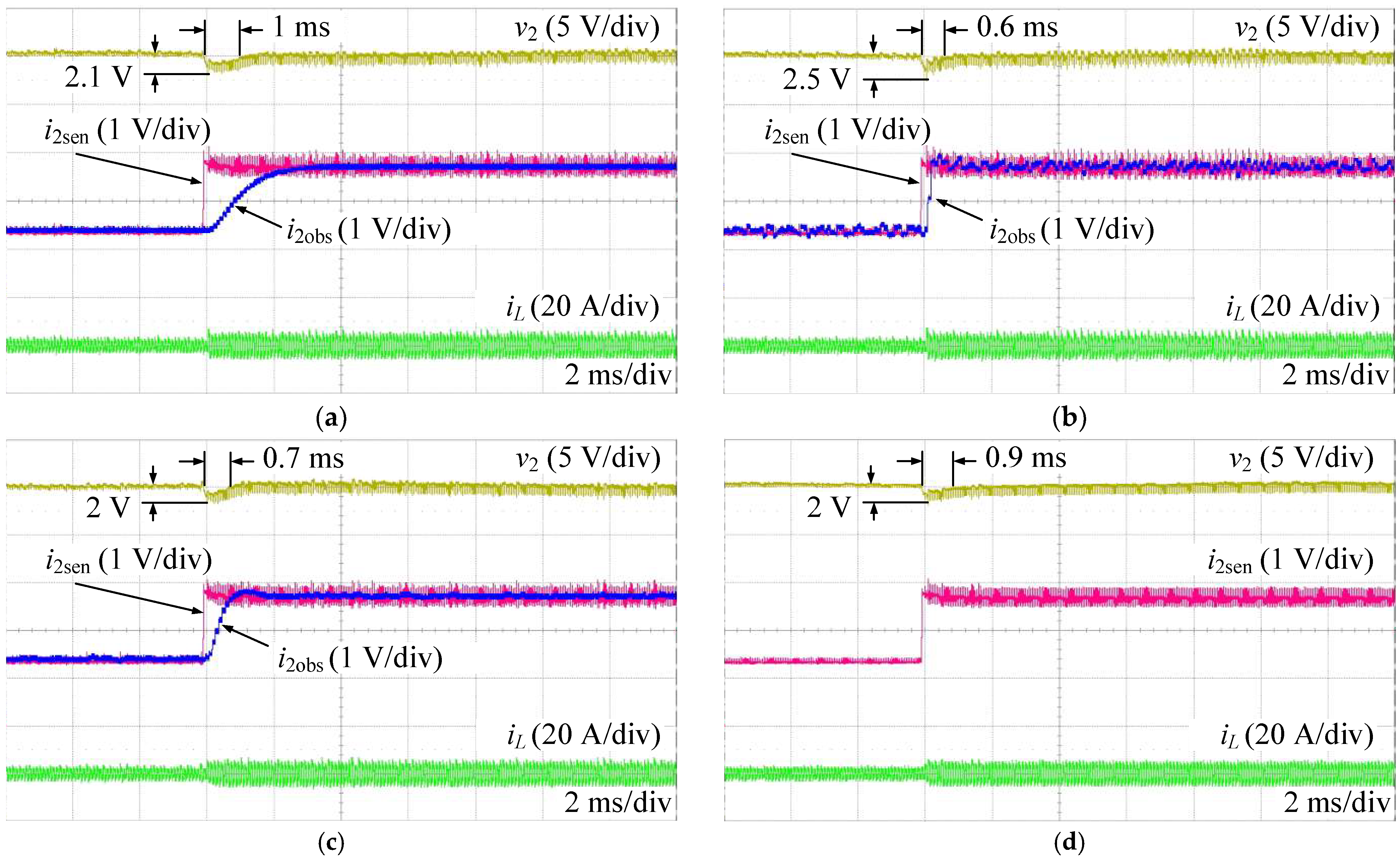
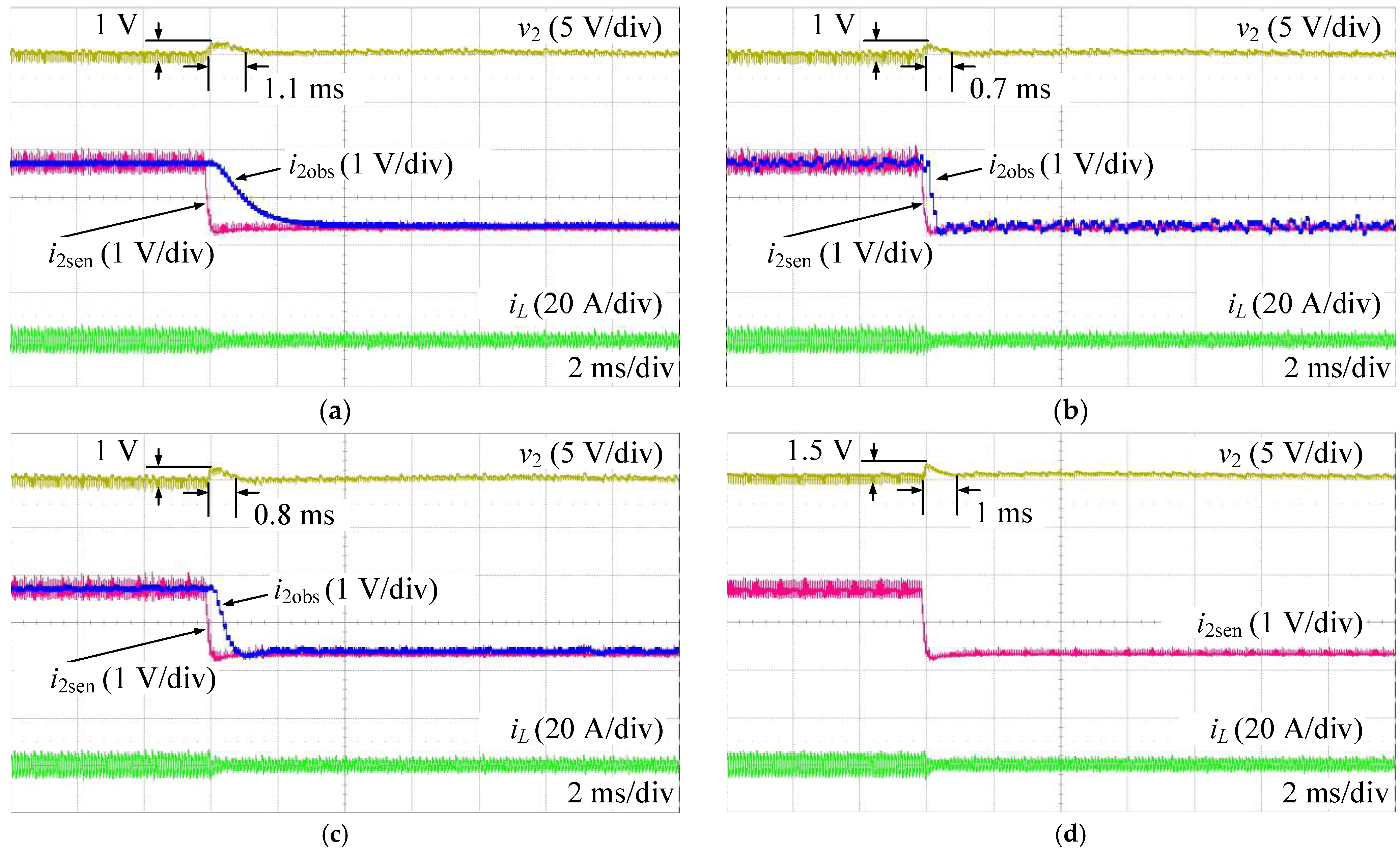
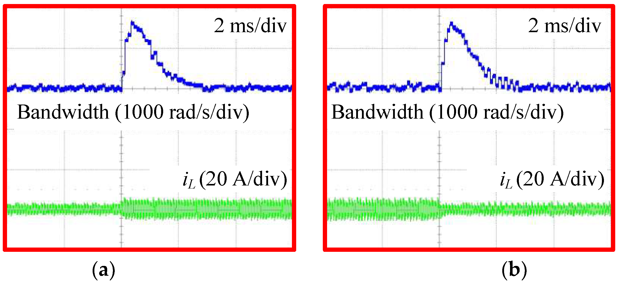
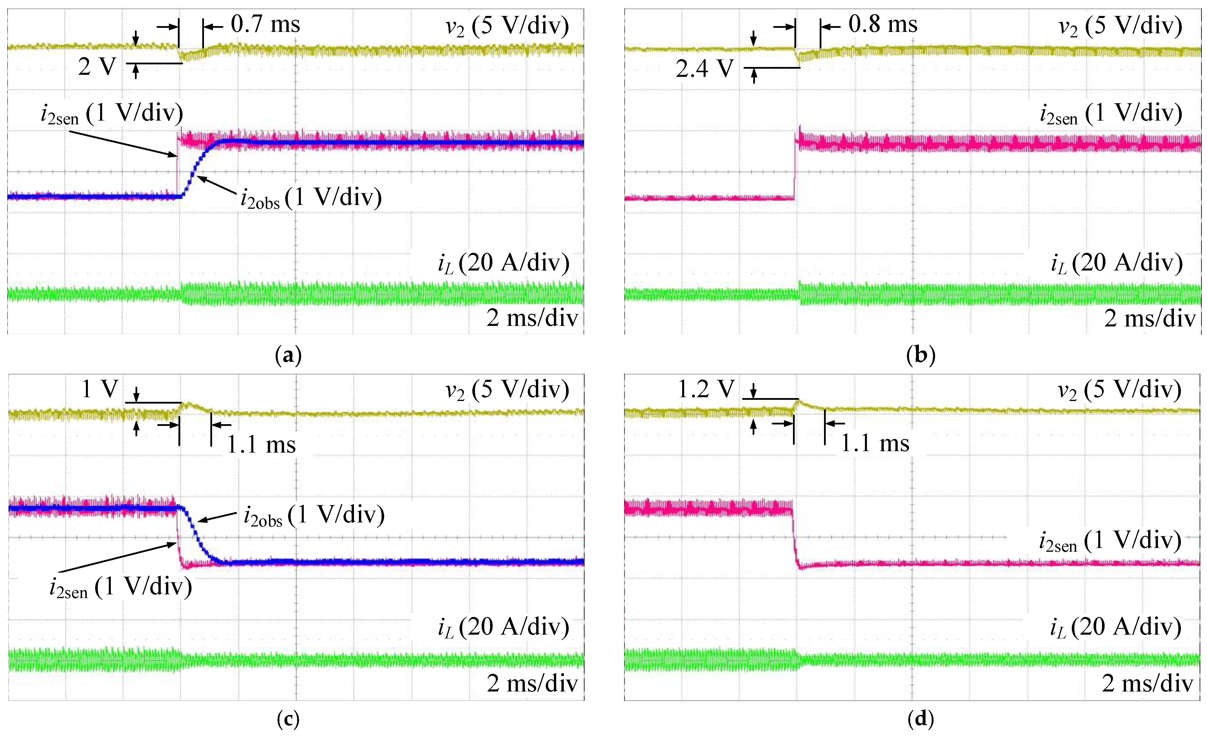
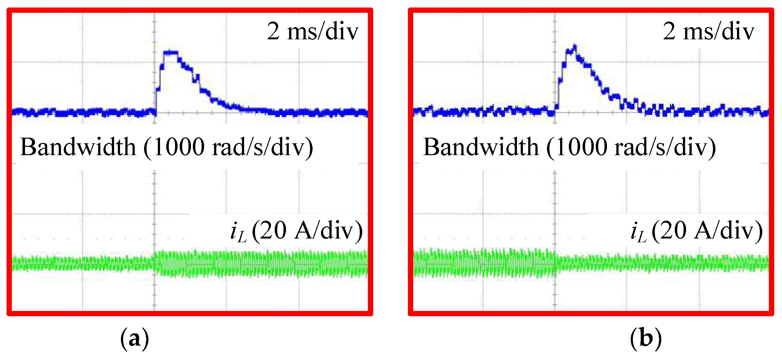
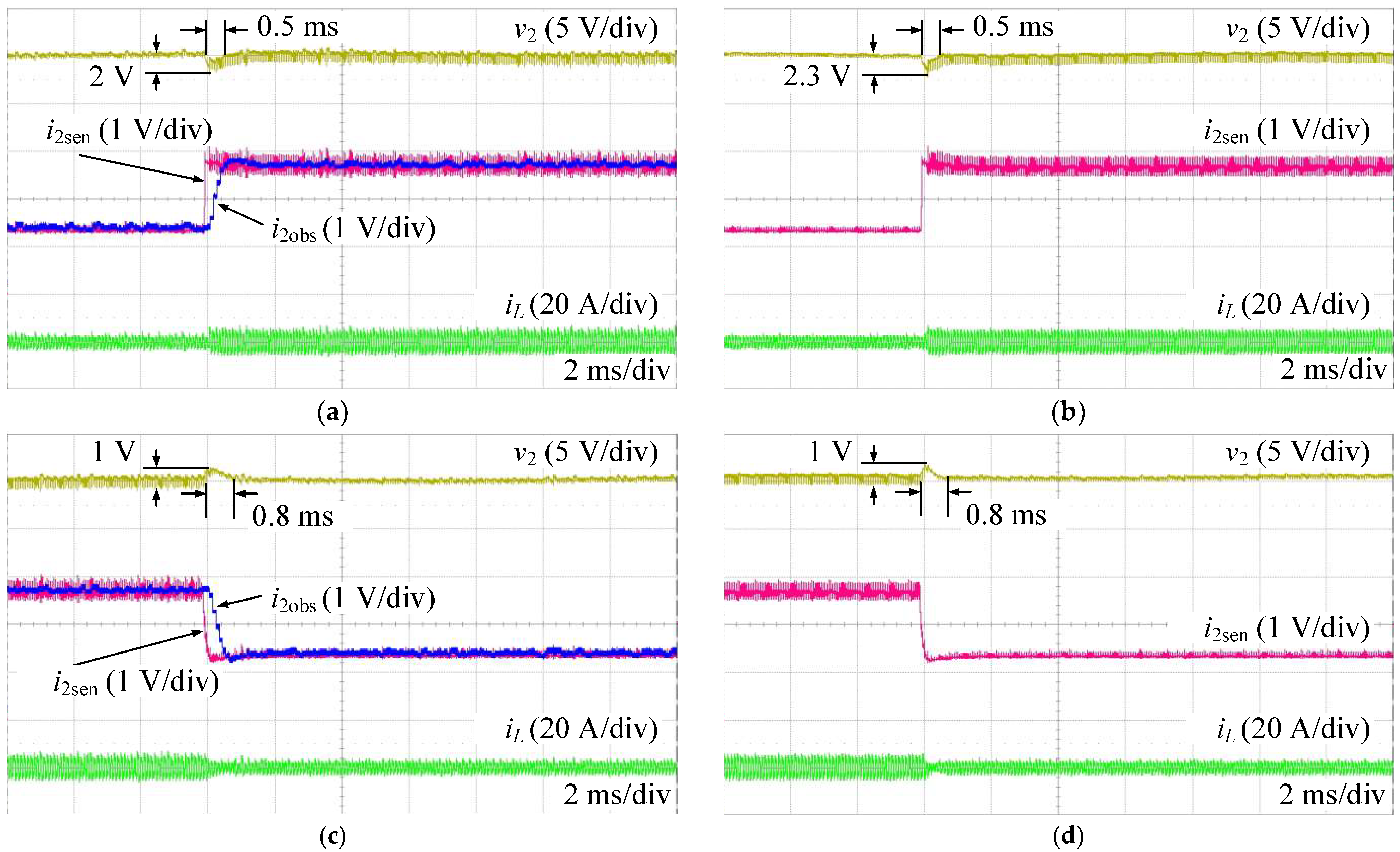
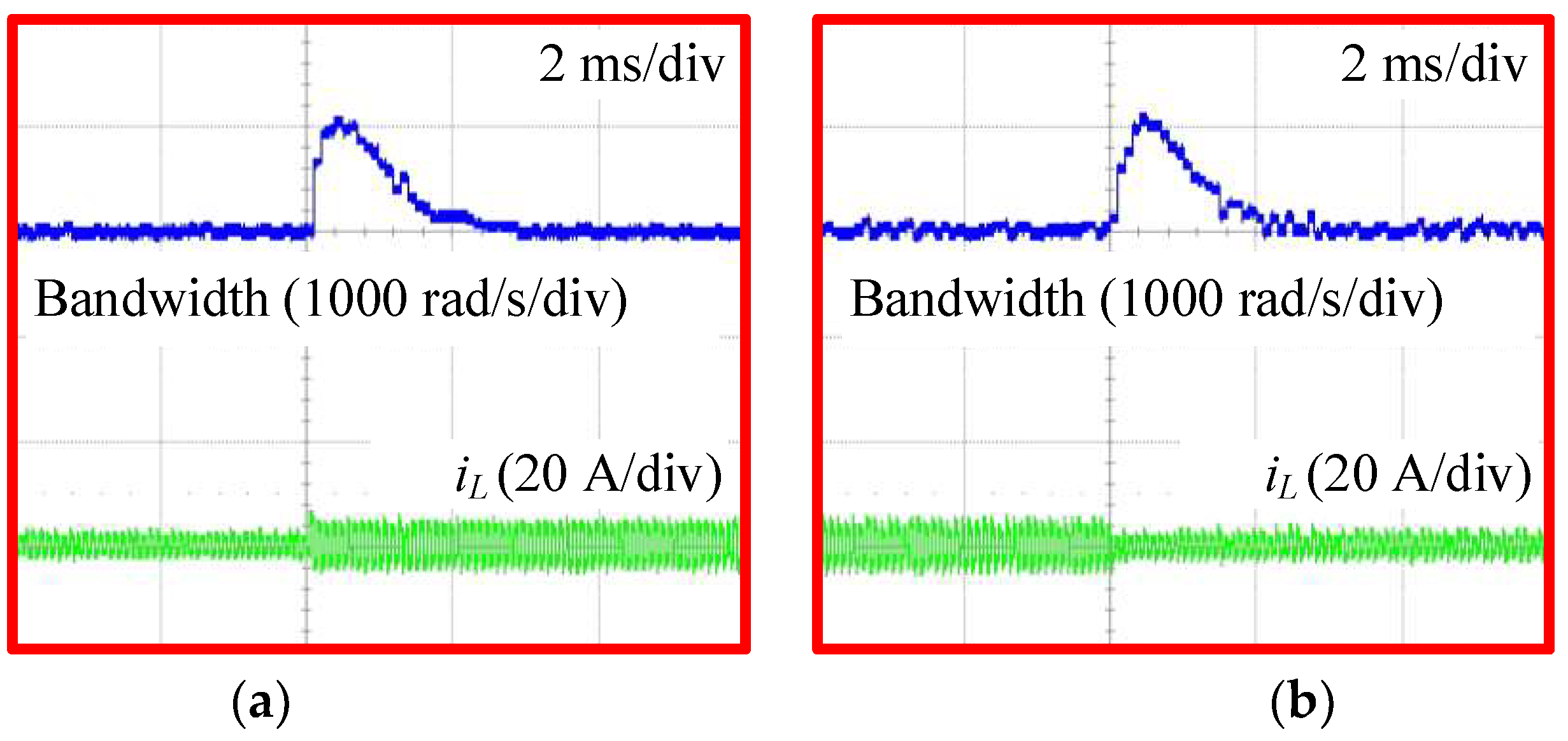
4.2. Experiment
5. Conclusions
Author Contributions
Funding
Institutional Review Board Statement
Informed Consent Statement
Data Availability Statement
Conflicts of Interest
Appendix A

| Symbol | Description | Value |
|---|---|---|
| Cutoff frequency | 2000π rad/s | |
| Phase margin | 60 deg | |
| Control delay | 50 μs | |
| Proportional gain | 1.376 | |
| Integrator time constant | 0.7488 ms |
References
- Hou, N.; Li, Y.W. Overview and Comparison of Modulation and Control Strategies for a Nonresonant Single-Phase Dual-Active-Bridge DC-DC Converter. IEEE Trans. Power Electron. 2020, 35, 3148–3172. [Google Scholar] [CrossRef]
- Zhao, B.; Song, Q.; Liu, W.; Sun, Y. Overview of dual-active-bridge isolated bidirectional DC-DC converter for high-frequency-link power-conversion system. IEEE Trans. Power Electron. 2014, 29, 4091–4106. [Google Scholar] [CrossRef]
- Shao, S.; Chen, L.; Shan, Z.; Gao, F.; Chen, H.; Sha, D.; Dragicevic, T. Modeling and Advanced Control of Dual-Active-Bridge DC-DC Converters: A Review. IEEE Trans. Power Electron. 2022, 37, 1524–1547. [Google Scholar] [CrossRef]
- Wang, J.; Wang, B.; Zhang, L.; Wang, J.; Shchurov, N.I.; Malozyomov, B.V. Review of bidirectional DC–DC converter topologies for hybrid energy storage system of new energy vehicles. Green Energy Intell. Transp. 2022, 1, 100010. [Google Scholar] [CrossRef]
- Xu, Q.; Vafamand, N.; Chen, L.; Dragicevic, T.; Xie, L.; Blaabjerg, F. Review on Advanced Control Technologies for Bidirectional DC/DC Converters in DC Microgrids. IEEE J. Emerg. Sel. Top. Power Electron. 2021, 9, 1205–1221. [Google Scholar] [CrossRef]
- Shao, S.; Chen, H.; Wu, X.; Zhang, J.; Sheng, K. Circulating Current and ZVS-on of a Dual Active Bridge DC-DC Converter: A Review. IEEE Access 2019, 7, 50561–50572. [Google Scholar] [CrossRef]
- Tong, A.; Hang, L.; Chung, H.S.H.; Li, G. Using Sampled-Data Modeling Method to Derive Equivalent Circuit and Linearized Control Method for Dual-Active-Bridge Converter. IEEE J. Emerg. Sel. Top. Power Electron. 2021, 9, 1361–1374. [Google Scholar] [CrossRef]
- Segaran, D.; Holmes, D.G.; McGrath, B.P. Enhanced load step response for a bidirectional DC-DC converter. IEEE Trans. Power Electron. 2013, 28, 371–379. [Google Scholar] [CrossRef]
- Song, W.; Hou, N.; Wu, M. Virtual Direct Power Control Scheme of Dual Active Bridge DC-DC Converters for Fast Dynamic Response. IEEE Trans. Power Electron. 2018, 33, 1750–1759. [Google Scholar] [CrossRef]
- Xiao, Q.; Chen, L.; Jia, H.; Wheeler, P.W.; Dragicevic, T. Model Predictive Control for Dual Active Bridge in Naval DC Microgrids Supplying Pulsed Power Loads Featuring Fast Transition and Online Transformer Current Minimization. IEEE Trans. Ind. Electron. 2020, 67, 5197–5203. [Google Scholar] [CrossRef]
- Chen, L.; Shao, S.; Xiao, Q.; Tarisciotti, L.; Wheeler, P.W.; Dragičević, T. Model Predictive Control for Dual-Active-Bridge Converters Supplying Pulsed Power Loads in Naval DC Micro-Grids. IEEE Trans. Power Electron. 2020, 35, 1957–1966. [Google Scholar] [CrossRef]
- Chen, L.; Lin, L.; Shao, S.; Gao, F.; Wang, Z.; Wheeler, P.W.; Dragicevic, T. Moving Discretized Control Set Model-Predictive Control for Dual-Active Bridge with the Triple-Phase Shift. IEEE Trans. Power Electron. 2020, 35, 8624–8637. [Google Scholar] [CrossRef]
- Chen, L.; Gao, F.; Shen, K.; Wang, Z.; Tarisciotti, L.; Wheeler, P.; Dragicevic, T. Predictive Control Based DC Microgrid Stabilization with the Dual Active Bridge Converter. IEEE Trans. Ind. Electron. 2020, 67, 8944–8956. [Google Scholar] [CrossRef]
- Tarisciotti, L.; Chen, L.; Shao, S.; Dragicevic, T.; Wheeler, P.; Zanchetta, P. Finite Control Set Model Predictive Control for Dual Active Bridge Converter. IEEE Trans. Ind. Appl. 2022, 58, 2155–2165. [Google Scholar] [CrossRef]
- Shan, Z.; Jatskevich, J.; Iu, H.H.C.; Fernando, T. Simplified load-feedforward control design for dual-active-bridge converters with current-mode modulation. IEEE J. Emerg. Sel. Top. Power Electron. 2018, 6, 2073–2085. [Google Scholar] [CrossRef]
- Dutta, S.; Bhattacharya, S.; Chandorkar, M. A novel predictive phase shift controller for bidirectional isolated dc to dc converter for high power applications. 2012 IEEE Energy Convers. Congr. Expo. ECCE 2012, 2012, 418–423. [Google Scholar] [CrossRef]
- Dutta, S.; Hazra, S.; Bhattacharya, S. A digital predictive current-mode controller for a single-phase high-frequency transformer-isolated dual-active bridge DC-to-DC converter. IEEE Trans. Ind. Electron. 2016, 63, 5943–5952. [Google Scholar] [CrossRef]
- Jeung, Y.C.; Lee, D.C. Voltage and current regulations of bidirectional isolated dual-active-bridge DC-DC converters based on a double-integral sliding mode control. IEEE Trans. Power Electron. 2019, 34, 6937–6946. [Google Scholar] [CrossRef]
- Li, K.; Yang, Y.; Tan, S.; Hui, R.S. Sliding-Mode-Based Direct Power Control of Dual-Active-Bridge DC-DC Converters. In Proceedings of the 2019 IEEE Applied Power Electronics Conference and Exposition (APEC), Anaheim, CA, USA, 17–21 March 2019; pp. 188–192. [Google Scholar]
- Tiwary, N.; Naik, N.V.; Panda, A.K.; Narendra, A.; Lenka, R.K. A Robust Voltage Control of DAB Converter with Super-Twisting Sliding Mode Approach. IEEE J. Emerg. Sel. Top. Ind. Electron. 2023, 4, 288–298. [Google Scholar] [CrossRef]
- Sun, J.; Qiu, L.; Liu, X.; Ma, J.; Fang, Y. Model-Free Moving-Discretized-Control-Set Predictive Control for Three-Phase Dual-Active-Bridge Converters. IEEE Trans. Power Electron. 2023, 1–15. [Google Scholar] [CrossRef]
- Zhao, W.; Zhang, X.; Gao, S.; Ma, M. Improved Model-Based Phase-Shift Control for Fast Dynamic Response of Dual-Active-Bridge. IEEE J. Emerg. Sel. Top. Power Electron. 2021, 9, 223–231. [Google Scholar] [CrossRef]
- Chen, W.H.; Yang, J.; Guo, L.; Li, S. Disturbance-Observer-Based Control and Related Methods—An Overview. IEEE Trans. Ind. Electron. 2016, 63, 1083–1095. [Google Scholar] [CrossRef]
- Sun, D. Comments on active disturbance rejection control. IEEE Trans. Ind. Electron. 2007, 54, 3428–3429. [Google Scholar] [CrossRef]
- Han, J. From PID to active disturbance rejection control. IEEE Trans. Ind. Electron. 2009, 56, 900–906. [Google Scholar] [CrossRef]
- Lakomy, K.; Madonski, R.; Dai, B.; Yang, J.; Kicki, P.; Ansari, M.; Li, S. Active Disturbance Rejection Control Design with Suppression of Sensor Noise Effects in Application to DC-DC Buck Power Converter. IEEE Trans. Ind. Electron. 2022, 69, 816–824. [Google Scholar] [CrossRef]
- Ahmad, S.; Ali, A. On Active Disturbance Rejection Control in Presence of Measurement Noise. IEEE Trans. Ind. Electron. 2022, 69, 11600–11610. [Google Scholar] [CrossRef]
- Wu, Y.; Yang, F. Saturated adaptive feedback control of electrical-optical gyro-stabilized platform based on cascaded adaptive extended state observer with complex disturbances. IET Control Theory Appl. 2023, 17, 1311–1330. [Google Scholar] [CrossRef]
- Liu, J.; An, H.; Gao, Y.; Wang, C.; Wu, L. Adaptive Control of Hypersonic Flight Vehicles with Limited Angle-of-Attack. IEEE/ASME Trans. Mechatron. 2018, 23, 883–894. [Google Scholar] [CrossRef]
- Zuo, Y.; Wang, H.; Ge, X.; Zuo, Y.; Woldegiorgis, A.T.; Feng, X.; Lee, C.H.T. A Novel Current Measurement Offset Error Compensation Method Based on the Adaptive Extended State Observer for IPMSM Drives. IEEE Trans. Ind. Electron. 2024, 71, 3371–3382. [Google Scholar] [CrossRef]
- Yue, J.; Liu, Z.; Su, H. Data-Driven Adaptive Extended State Observer-Based Model-Free Disturbance Rejection Control for DC–DC Converters. IEEE Trans. Ind. Electron. 2023, 1–11. [Google Scholar] [CrossRef]
- Yue, F.; Li, X.; Zhang, S. Robust Adaptive Integral Sliding Mode Control for Two-Axis Optoelectronic Tracking and Measuring System Based on Novel Nonlinear Extended State Observer. IEEE Trans. Instrum. Meas. 2023, 72, 1–11. [Google Scholar] [CrossRef]
- Luo, M.; Yu, Z.; Xiao, Y.; Xiong, L.; Xu, Q.; Ma, L.; Wu, Z. Full-order adaptive sliding mode control with extended state observer for high-speed PMSM speed regulation. Sci. Rep. 2023, 13, 6200. [Google Scholar] [CrossRef] [PubMed]
- Wang, J.; Liu, Y.; Yang, J.; Wang, F.; Rodriguez, J. Adaptive Integral Extended State Observer-Based Improved Multistep FCS-MPCC for PMSM. IEEE Trans. Power Electron. 2023, 38, 11260–11276. [Google Scholar] [CrossRef]
- Zheng, C.; Dragicevic, T.; Blaabjerg, F. Current-sensorless finite-set model predictive control for LC-Filtered voltage source inverters. IEEE Trans. Power Electron. 2020, 35, 1086–1095. [Google Scholar] [CrossRef]
- Zhang, H.; Li, Y.; Li, Z.; Zhao, C.; Gao, F.; Xu, F.; Wang, P. Extended-State-Observer Based Model Predictive Control of a Hybrid Modular DC Transformer. IEEE Trans. Ind. Electron. 2022, 69, 1561–1572. [Google Scholar] [CrossRef]
- Zhang, Y.; Jin, J.; Huang, L. Model-Free Predictive Current Control of PMSM Drives Based on Extended State Observer Using Ultralocal Model. IEEE Trans. Ind. Electron. 2021, 68, 993–1003. [Google Scholar] [CrossRef]
- Li, S.; Yang, J.; Chen, W.H.; Chen, X. Disturbance Observer-Based Control: Methods and Applications, 1st ed.; CRC Press: Boca Raton, FL, USA, 2014. [Google Scholar]
- Duong, T.Q.; Choi, S.J. Sensor-Reduction Control for Dual Active Bridge Converter Under Dual-Phase-Shift Modulation. IEEE Access 2022, 10, 63020–63033. [Google Scholar] [CrossRef]
- Gualous, H.; Bouquain, D.; Berthon, A.; Kauffmann, J.M. Experimental study of supercapacitor serial resistance and capacitance variations with temperature. J. Power Sources 2003, 123, 86–93. [Google Scholar] [CrossRef]
- Wilson, P. The Circuit Designer’s Companion, 3rd ed.; Newnes: Oxford, UK, 2012; ISBN 9780081017647. [Google Scholar]
- Texas Instruments. Analog—Passive Devices Application Report; Texas Instruments: Dallas, TX, USA, 1999. [Google Scholar]


| Symbol | Description | Value |
|---|---|---|
| Input voltage | 100 V | |
| Output voltage reference | 100 V | |
| Transformer turn ratio | 1 | |
| Switching frequency | 10 kHz | |
| Series inductance | 50 μH | |
| Input capacitance | 440 μF | |
| Output capacitance | 220 μF | |
| Resistive load | 50 Ω |
| Symbol | Description | Value |
|---|---|---|
| Minimum observer bandwidth | 500 rad/s | |
| Maximum observer bandwidth | 2500 rad/s | |
| Positive coefficient | 0.1 |
| Component | Description | Value |
|---|---|---|
| Switching devices | C3M0065090D × 8 | VDS = 900 V, ID = 36 A |
| Input capacitors | Panasonic UQ Samyoung TDA | 450 V, 220 μF 450 V, 220 μF |
| Output capacitors | Samyoung TDA | 450 V, 220 μF |
| Transformer | TDK PQ50/50, Ferrite Core, Litz wire 0.1 mm × 140 strands | 31:31 turns |
| Inductor | TDK EI40, Ferrite Core, Litz wire 0.1 mm × 140 strands | 24 turns |
| Voltage sensors | LV 25-P | t = 40 μs |
| Current sensors | LA 55-P | BW (–1 dB) 200 kHz |
| Symbol | Description | Value |
|---|---|---|
| Input voltage | 80 V | |
| Output voltage reference | 80 V | |
| Transformer turn ratio | 1 | |
| Switching frequency | 10 kHz | |
| Series inductance | 51 μH | |
| Input capacitance | 431 μF | |
| Output capacitance | 219 μF | |
| Resistive load | 57 Ω |
| Validation | Operation Scenario | Overshoot/Undershoot | Settling Time | ||||||
|---|---|---|---|---|---|---|---|---|---|
| LESO | HESO | AESO | MPSC | LESO | HESO | AESO | MPSC | ||
| Simulation | Changing the load current | 1 V | 1 V | 1 V | 1.2 V | 4 ms | 3 ms | 2 ms | 4 ms |
| Changing the voltage reference | 0.2 V | 0.4 V | 0.2 V | 1.2 V | 1 ms | 1 ms | 1 ms | 4 ms | |
| Changing the input voltage | 1.2 V | 1.2 V | 1.2 V | 1.25 V | 0.1 ms | 0.1 ms | 0.1 ms | 1.5 ms | |
| Experiment | Increasing the load current | 2.1 V | 2.5 V | 2 V | 2 V | 1 ms | 0.6 ms | 0.7 ms | 0.9 ms |
| Decreasing the load current | 1 V | 1 V | 1 V | 1.5 V | 1.1 ms | 0.7 ms | 0.8 ms | 1 ms | |
| Tasks | MPSC | AESO |
|---|---|---|
| Number of current sensors | 2 | 0 |
| Number of voltage sensors | 2 | 2 |
| Observer performance | - | Good |
| Dynamic performance | Moderate | Good |
| Robustness to parameter mismatches | Moderate | Good |
Disclaimer/Publisher’s Note: The statements, opinions and data contained in all publications are solely those of the individual author(s) and contributor(s) and not of MDPI and/or the editor(s). MDPI and/or the editor(s) disclaim responsibility for any injury to people or property resulting from any ideas, methods, instructions or products referred to in the content. |
© 2024 by the authors. Licensee MDPI, Basel, Switzerland. This article is an open access article distributed under the terms and conditions of the Creative Commons Attribution (CC BY) license (https://creativecommons.org/licenses/by/4.0/).
Share and Cite
Duong, T.-Q.; Trinh, H.-A.; Ahn, K.-K.; Choi, S.-J. Adaptive Extended State Observer for the Dual Active Bridge Converters. Sensors 2024, 24, 2397. https://doi.org/10.3390/s24082397
Duong T-Q, Trinh H-A, Ahn K-K, Choi S-J. Adaptive Extended State Observer for the Dual Active Bridge Converters. Sensors. 2024; 24(8):2397. https://doi.org/10.3390/s24082397
Chicago/Turabian StyleDuong, Tan-Quoc, Hoai-An Trinh, Kyoung-Kwan Ahn, and Sung-Jin Choi. 2024. "Adaptive Extended State Observer for the Dual Active Bridge Converters" Sensors 24, no. 8: 2397. https://doi.org/10.3390/s24082397
APA StyleDuong, T.-Q., Trinh, H.-A., Ahn, K.-K., & Choi, S.-J. (2024). Adaptive Extended State Observer for the Dual Active Bridge Converters. Sensors, 24(8), 2397. https://doi.org/10.3390/s24082397