
LSTM Short-Term Wind Power Prediction Method Based on Data Preprocessing and Variational Modal Decomposition for Soft Sensors

Abstract
:1. Introduction
2. Method
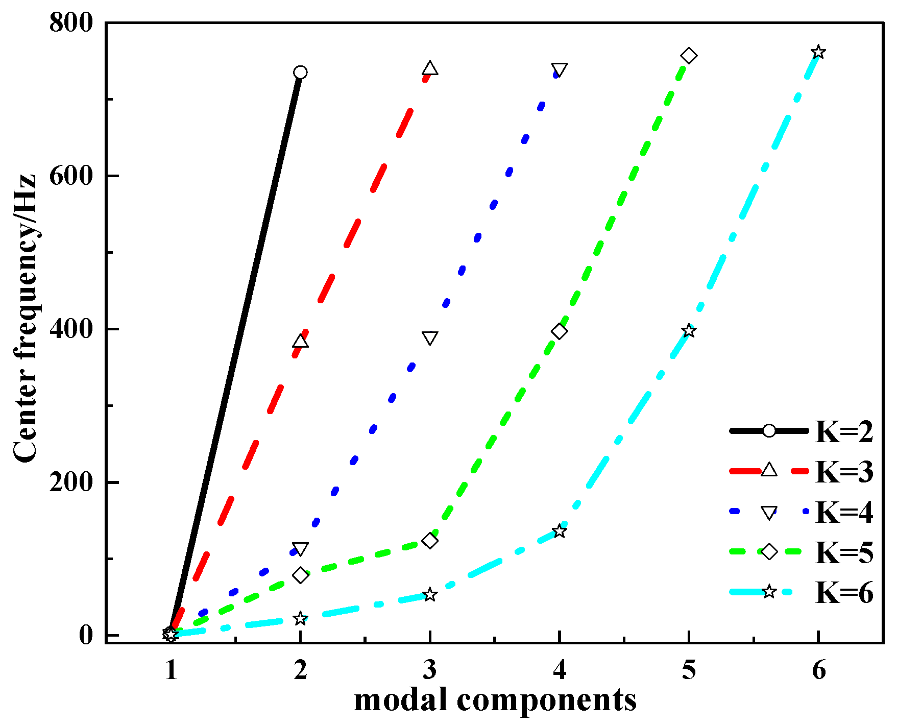
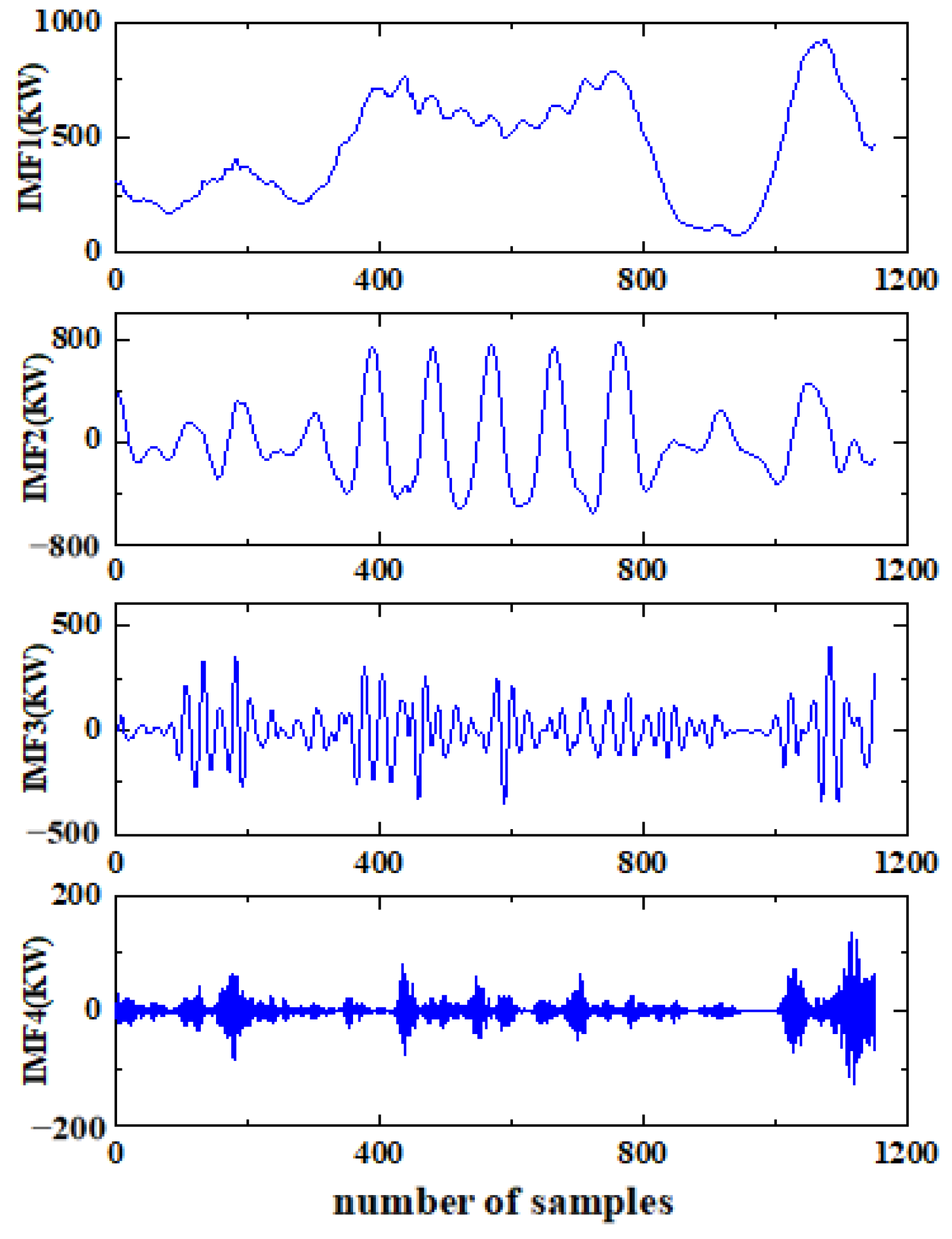
2.1. VMD
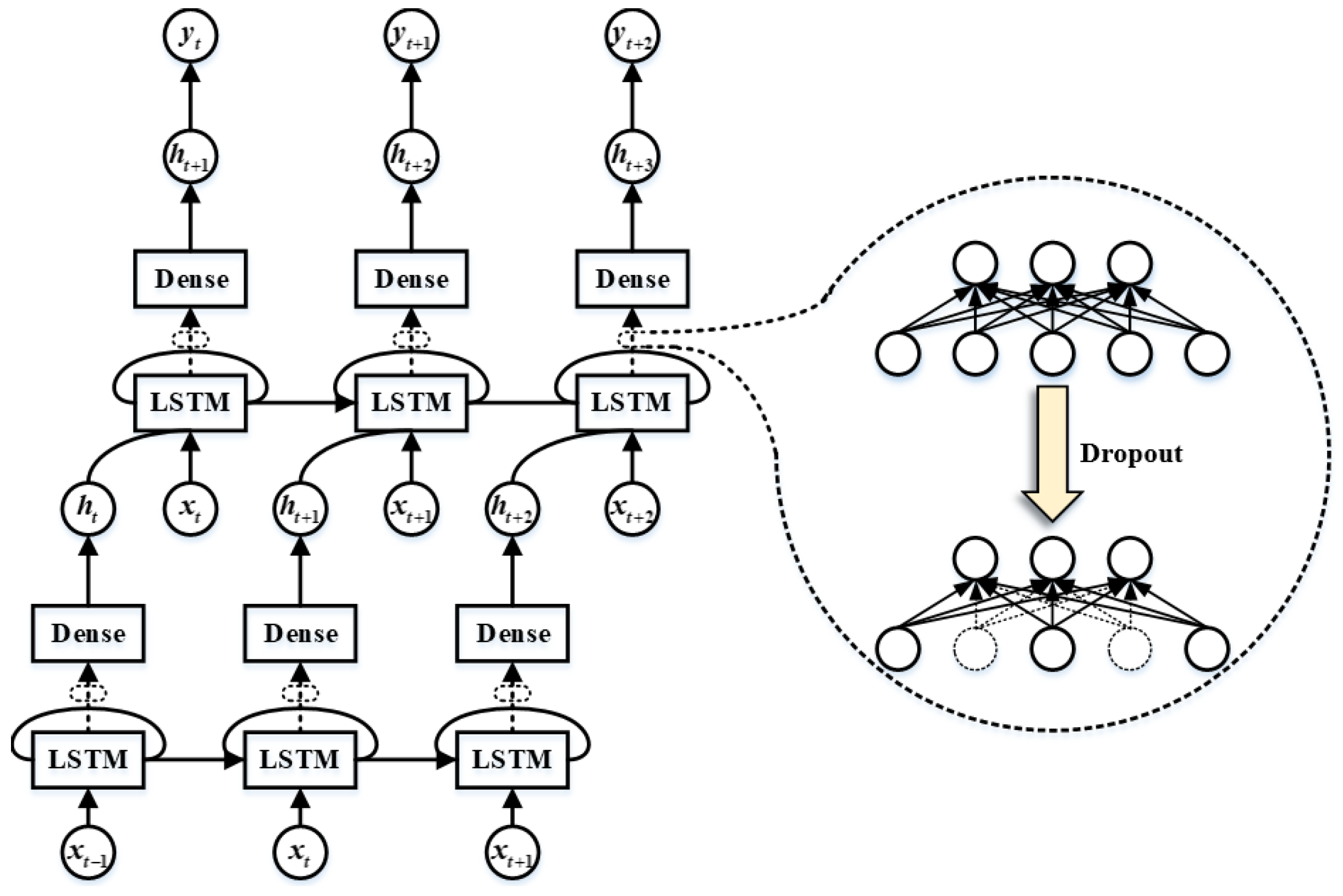
2.2. LSTM
3. Results and Analysis
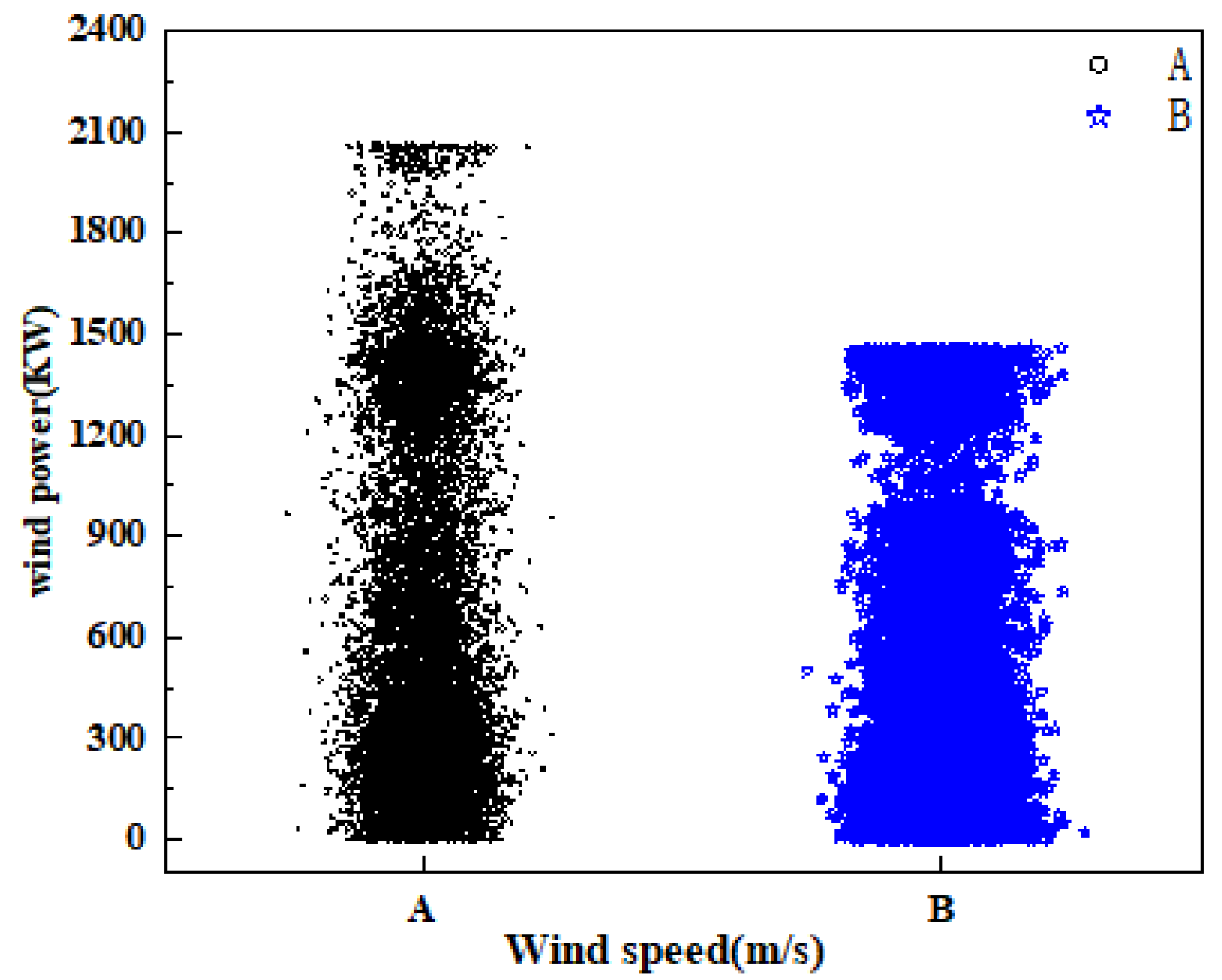
3.1. Experimental Data and Evaluation Indicators
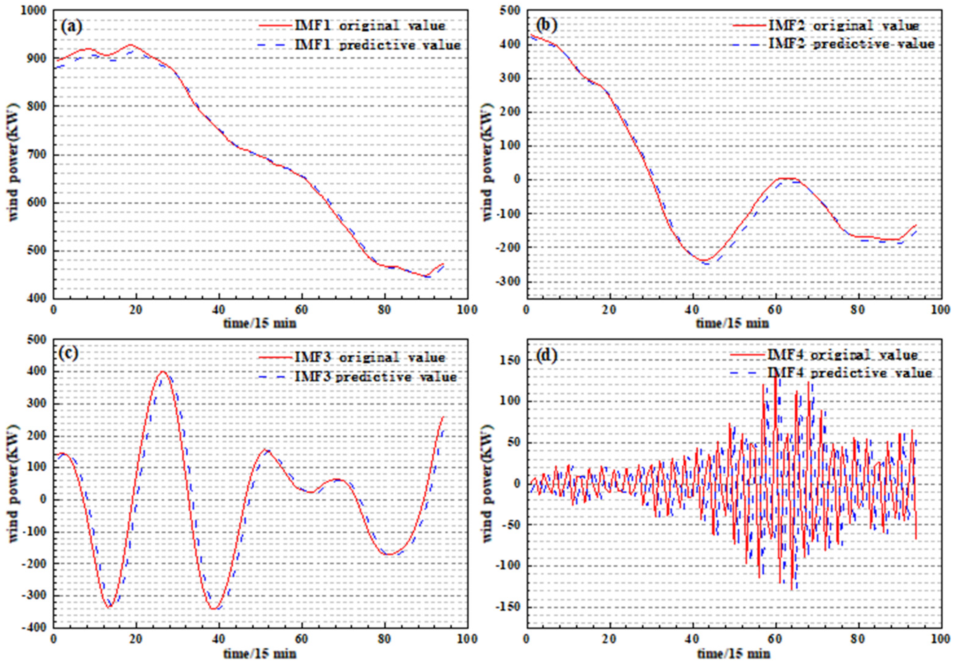
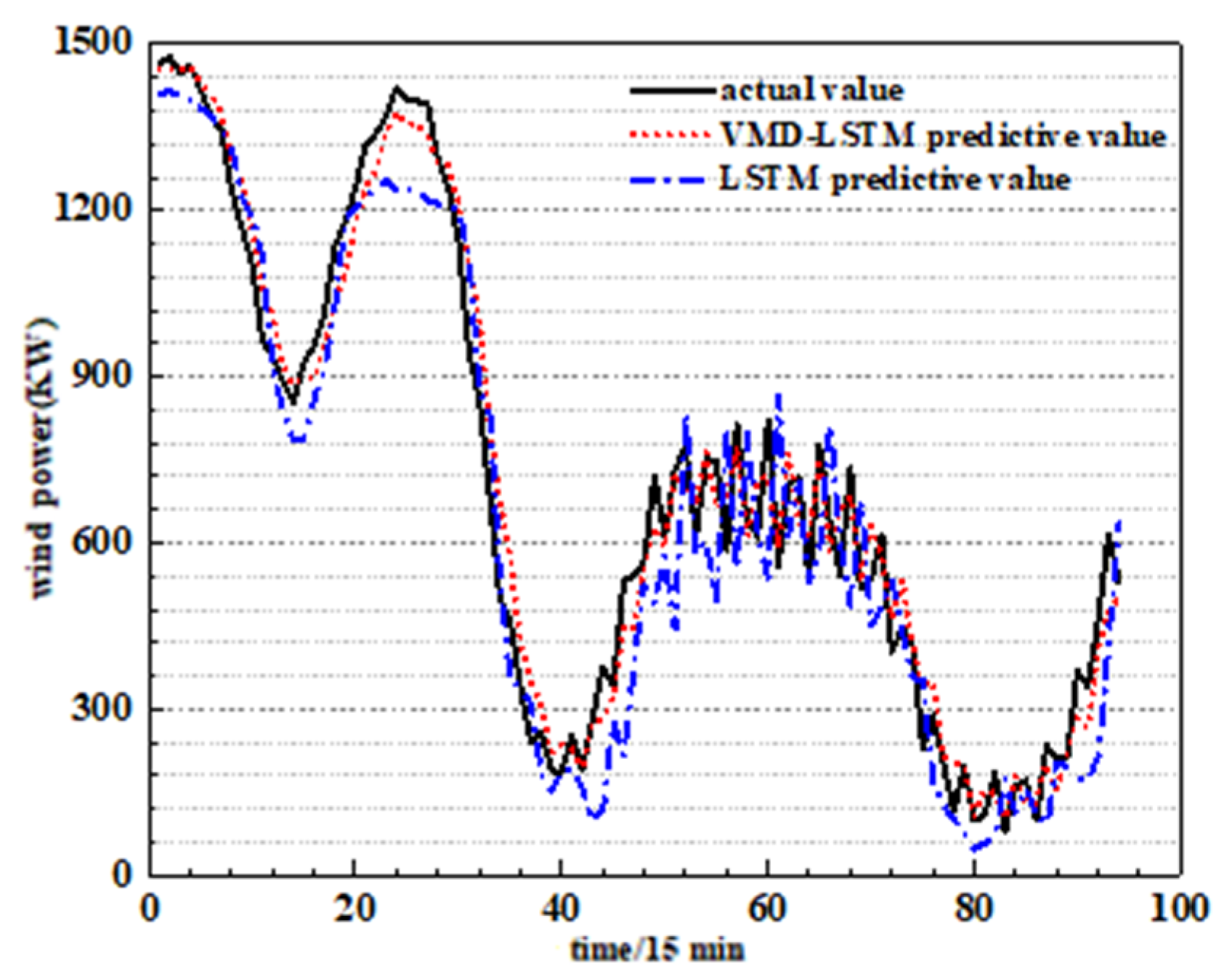
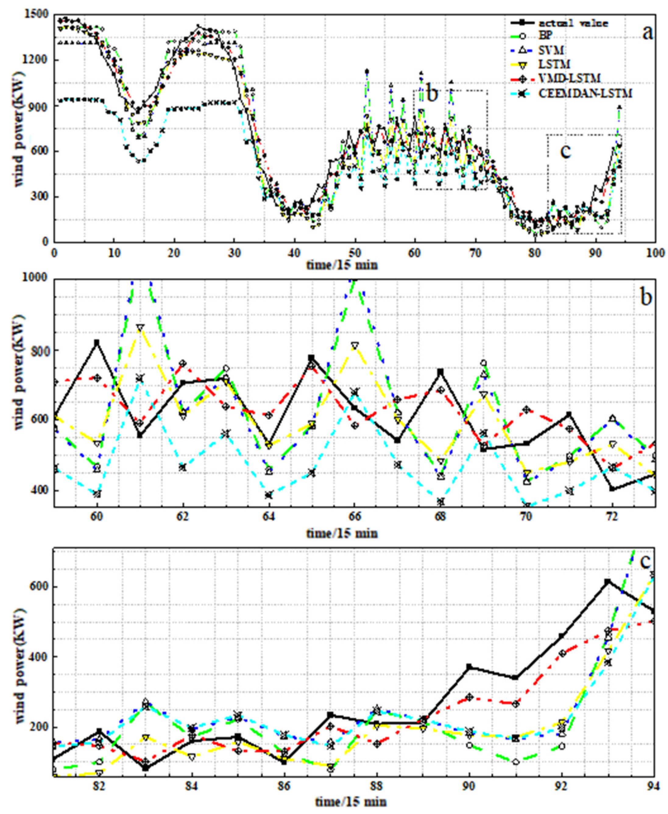
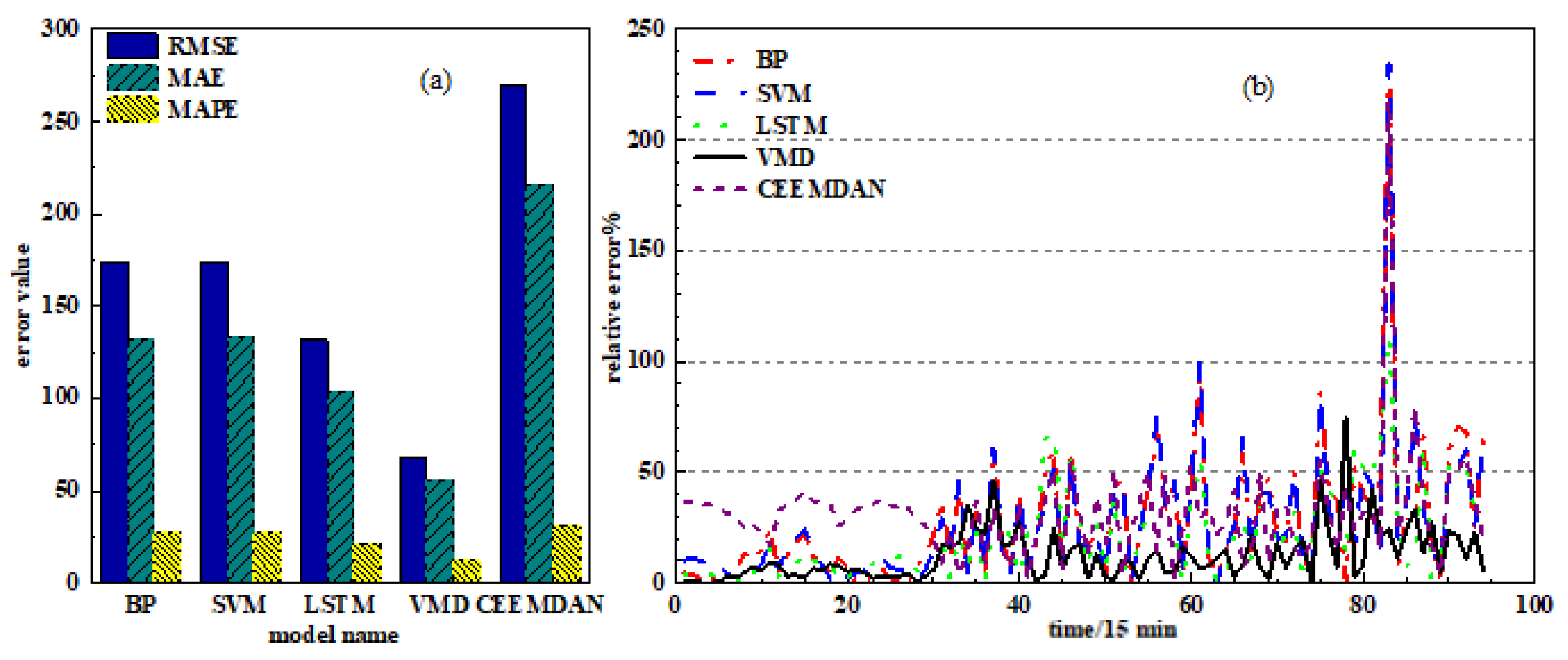
3.2. Data Preprocessing and Result Analysis
4. Conclusions
- Using the isolated forest algorithm to detect anomalies in the original wind power sequence and to perform multiple imputation processing on missing data.
- In terms of data processing, the experimental data is processed using the minimum-maximum normalization (MMN) method for dimensionless data, and the data values are mapped to the [0, 1] interval, which improves the effectiveness of data processing.
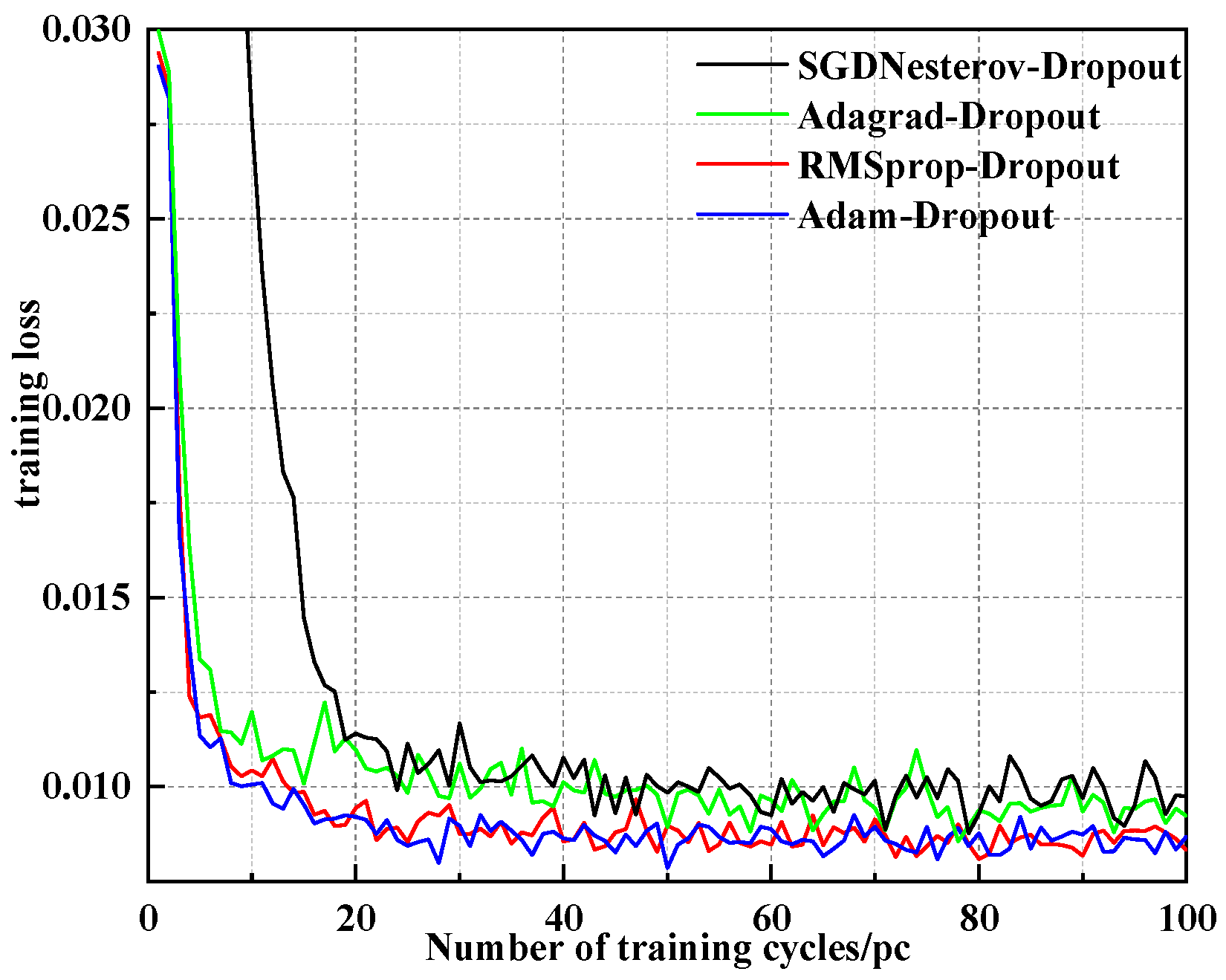
- Compared with the RMSProp algorithm, Adagrad algorithm and SGD Nesterov algorithm, using the Adam algorithm to optimize LSTM network parameters has better convergence accuracy.
- The VMD method has better decomposition results than the CEEMDAN method because its own Wiener filter can effectively complete the noise reduction and prevent modal aliasing.
- Compared with traditional BPNN and SVM, LSTM is suitable for short-term wind power prediction and has better prediction accuracy.
Author Contributions
Funding
Institutional Review Board Statement
Informed Consent Statement
Data Availability Statement
Conflicts of Interest
References
- Wang, J.; Zhu, H.; Zhang, Y.; Cheng, F.; Zhou, C. A novel prediction model for wind power based on improved long short-term memory neural network. Energy 2023, 265, 126283. [Google Scholar] [CrossRef]
- Zheng, H.; Hu, Z.; Wang, X.; Nie, J.; Cui, M. VMD-CAT: A hybrid model for short-term wind power prediction. Energy Rep. 2023, 9, 199–211. [Google Scholar] [CrossRef]
- Hu, X.; Yu, Q.; Han, Y.; Chen, Z.; Geng, Z. Novel complex-valued long short-term memory network integrating variational mode decomposition for soft sensor. J. Process Control. 2023, 129, 103053. [Google Scholar] [CrossRef]
- Ahmed, A.; Khalid, M. A review on the selected applications of forecasting models in renewable power systems. Renew. Sustain. Energy Rev. 2019, 100, 9–21. [Google Scholar] [CrossRef]
- Zhang, Y.; Le, J.; Liao, X.; Feng, Z. A novel combination forecasting model for wind power integrating least square support vector machine, deep belief network, singular spectrum analysis and locality-sensitive hashing. Energy 2019, 168, 558–572. [Google Scholar] [CrossRef]
- Puggini, L.; Seán, M. An enhanced variable selection and Isolation Forest based methodology for anomaly detection with OES data. Eng. Appl. Artif. Intell. 2018, 67, 126–135. [Google Scholar] [CrossRef]
- Parri, S.; Teeparthi, K.; Kosana, V. A hybrid methodology using VMD and disentangled features for wind speed forecasting. Energy 2024, 288, 0360–5442. [Google Scholar] [CrossRef]
- Chen, H.; Wu, H.; Kan, T.; Zhang, J.; Li, H. Low-carbon economic dispatch of integrated energy system containing electric hydrogen production based on VMD-GRU short-term wind power prediction. Int. J. Electr. Power Energy Syst. 2023, 154, 109420. [Google Scholar] [CrossRef]
- Zhao, Z.; Yun, S.; Jia, L.; Guo, J.; Meng, Y.; He, N.; Yang, L. Hybrid VMD-CNN-GRU-based model for short-term forecasting of wind power considering spatio-temporal features. Eng. Appl. Artif. Intell. 2023, 121, 105982. [Google Scholar] [CrossRef]
- Huang, N.; Yuan, C.; Cai, G.; Xing, E. Hybrid Short Term Wind Speed Forecasting Using Variational Mode Decomposition and a Weighted Regularized Extreme Learning Machine. Energies 2016, 9, 989. [Google Scholar] [CrossRef]
- Pascanu, R.; Mikolov, T.; Bengio, Y. On the difficulty of training Recurrent Neural Networks. In Proceedings of the 30th International Conference on Machine Learning, Atlanta, GA, USA, 16–21 June 2013; pp. 1310–1318. [Google Scholar]
- Guan, S.; Wang, Y.; Liu, L.; Gao, J.; Xu, Z.; Kan, S. Ultra-short-term wind power prediction method based on FTI-VACA-XGB model. Expert Syst. Appl. 2024, 235, 121185. [Google Scholar] [CrossRef]
- Yin, L.; Zhao, M. Inception-embedded attention memory fully-connected network for short-term wind power prediction. Appl. Soft Comput. 2023, 141, 110279. [Google Scholar] [CrossRef]
- Yang, S.; Yuan, A.; Yu, Z. A novel model based on CEEMDAN, IWOA, and LSTM for ultra-short-term wind power forecasting. Environ. Sci. Pollut. Res. 2023, 235, 11689–11705. [Google Scholar] [CrossRef] [PubMed]
- Erick, L.; Carlos, V.; Héctor, A.; Esteban, G.; Henrik, M. Wind Power Forecasting Based on Echo State Networks and Long Short-Term Memory. Energies 2018, 11, 526. [Google Scholar] [CrossRef]
- Yu, C.; Li, Y.; Bao, Y.; Tang, H.; Zhai, G. A novel framework for wind speed prediction based on recurrent neural networks and support vector machine. Energy Convers. Manag. 2018, 178, 137–145. [Google Scholar] [CrossRef]
- Curreri, F.; Patanè, L.; Gabriella Xibilia, M. RNN- and LSTM-Based Soft Sensors Transferability for an Industrial Process. Sensors 2021, 21, 823. [Google Scholar] [CrossRef] [PubMed]
- Zhang, F.; Li, N.; Li, L.; Wang, S.; Du, C. A local semi-supervised ensemble learning strategy for the data-driven soft sensor of the power prediction in wind power generation. Fuel 2023, 333, 126435. [Google Scholar] [CrossRef]
- Li, H.; Jing, H.; Zhang, R.; Gao, Z. Wind power forecast based on improved Long Short Term Memory Network. Energy 2019, 189, 116300. [Google Scholar]
- Yu, M.; Niu, D.; Gao, T.; Wang, K.; Sun, L.; Li, M.; Xu, X. A novel framework for ultra-short-term interval wind power prediction based on RF-WOA-VMD and BiGRU optimized by the attention mechanism. Energy 2023, 269, 126738. [Google Scholar] [CrossRef]
- Abou Houran, M.; Bukhari, S.M.S.; Zafar, M.H.; Mansoor, M.; Chen, W. COA-CNN-LSTM: Coati optimization algorithm-based hybrid deep learning model for PV/wind power forecasting in smart grid applications. Appl. Energy 2023, 349, 121638. [Google Scholar] [CrossRef]
- Liu, T.; Ting, K.; Zhou, Z. Spectrum of variable-random trees. J. Artif. Intell. Res. 2008, 32, 355–384. [Google Scholar] [CrossRef]
- Dragomiretskiy, K.; Zosso, D. Variational Mode Decomposition. IEEE Trans. Signal Process. 2014, 62, 531–544. [Google Scholar] [CrossRef]
- Gal, Y.; Ghahramani, Z.B.A. Theoretically Grounded Application of Dropout in Recurrent Neural Networks. Statistics 2016, 29, 285–290. [Google Scholar]
- Duan, J.; Wang, P.; Ma, W.; Tian, X.; Fang, S.; Chen, Y.; Chang, Y.; Liu, H. Short-term wind power forecasting using the hybrid model of improved variational mode decomposition and Correntropy Long Short -term memory neural network. Energy 2021, 214, 118980. [Google Scholar] [CrossRef]
- Liu, W.; Liu, Y.; Fu, L.; Yang, M.; Hu, R. Wind Power Forecasting Method Based on Bidirectional Long Short-Term Memory Neural Network and Error Correction. Electr. Power Compon. Syst. 2022, 49, 1169–1180. [Google Scholar] [CrossRef]
- Hu, X.; Ma, L. Application of VMD-LSTM algorithm in short term load forecasting. Electr. Power Sci. Eng. 2018, 34, 9. [Google Scholar]
- Wang, J.; Li, X.; Zhou, X.; Zhang, K. Ultra-short-term wind speed prediction based on VMD-LSTM. Power Syst. Prot. Control. 2020, 34, 45–52. [Google Scholar]


| Modal Number | Center Frequency/Hz | |||||
|---|---|---|---|---|---|---|
| IMF1 | IMF2 | IMF3 | IMF4 | IMF5 | IMF6 | |
| 2 | 2.81 | 735.23 | ||||
| 3 | 1.43 | 382.21 | 738.86 | |||
| 4 | 1.22 | 114.96 | 390.34 | 740.88 | ||
| 5 | 1.08 | 78.47 | 123.54 | 396.97 | 757.22 | |
| 6 | 0.97 | 21.63 | 52.69 | 135.72 | 397.42 | 761.53 |
| Modal Number | C12 | C23 | C34 | C45 | C56 |
|---|---|---|---|---|---|
| 2 | 0.0915 | ||||
| 3 | 0.0618 | 0.0900 | |||
| 4 | 0.0519 | 0.0901 | 0.0963 | ||
| 5 | 0.3614 | 0.2906 | 0.0257 | 0.0810 | |
| 6 | 0.3501 | 0.2860 | 0.1284 | 0.0284 | 0.0601 |
| BP | SVM | LSTM | VMD-LSTM | CEEMDAN-LSTM | |
|---|---|---|---|---|---|
| RMSE (KW) | 173.8774 | 174.0292 | 131.6665 | 67.6993 | 270.0046 |
| MAE (KW) | 131.4138 | 133.1894 | 103.9460 | 55.7662 | 215.4398 |
| MAPE (%) | 26.9278 | 26.8527 | 21.4184 | 12.0676 | 31.4652 |
Disclaimer/Publisher’s Note: The statements, opinions and data contained in all publications are solely those of the individual author(s) and contributor(s) and not of MDPI and/or the editor(s). MDPI and/or the editor(s) disclaim responsibility for any injury to people or property resulting from any ideas, methods, instructions or products referred to in the content. |
© 2024 by the authors. Licensee MDPI, Basel, Switzerland. This article is an open access article distributed under the terms and conditions of the Creative Commons Attribution (CC BY) license (https://creativecommons.org/licenses/by/4.0/).
Share and Cite
Lei, P.; Ma, F.; Zhu, C.; Li, T. LSTM Short-Term Wind Power Prediction Method Based on Data Preprocessing and Variational Modal Decomposition for Soft Sensors. Sensors 2024, 24, 2521. https://doi.org/10.3390/s24082521
Lei P, Ma F, Zhu C, Li T. LSTM Short-Term Wind Power Prediction Method Based on Data Preprocessing and Variational Modal Decomposition for Soft Sensors. Sensors. 2024; 24(8):2521. https://doi.org/10.3390/s24082521
Chicago/Turabian StyleLei, Peng, Fanglan Ma, Changsheng Zhu, and Tianyu Li. 2024. "LSTM Short-Term Wind Power Prediction Method Based on Data Preprocessing and Variational Modal Decomposition for Soft Sensors" Sensors 24, no. 8: 2521. https://doi.org/10.3390/s24082521