

Mind the Exit Pupil Gap: Revisiting the Intrinsics of a Standard Plenoptic Camera


Abstract
1. Introduction

- A formal deduction of the connection between object distance and sub-aperture image shift considering the exit pupil.
- A model for the errors resulting from ignoring the exit pupil in this relation.
1.1. Related Work
1.2. Organization
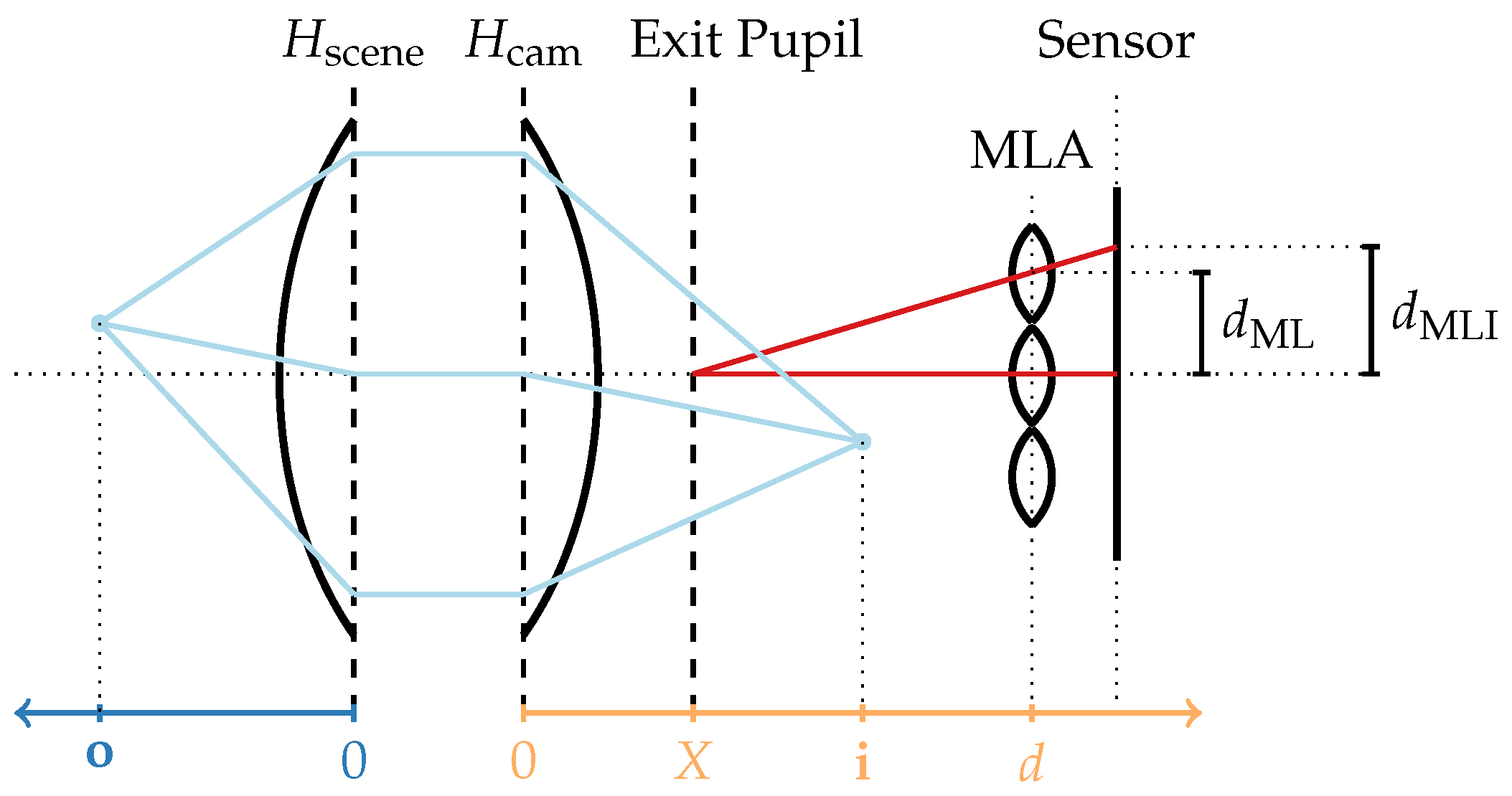
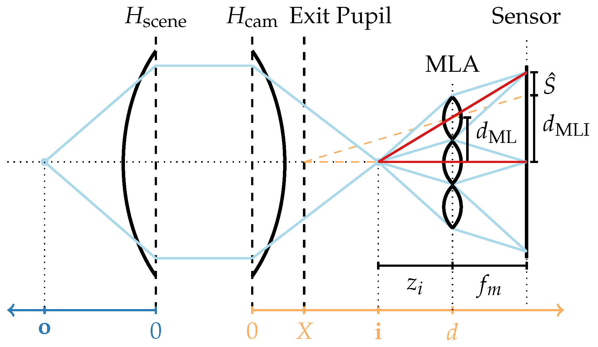
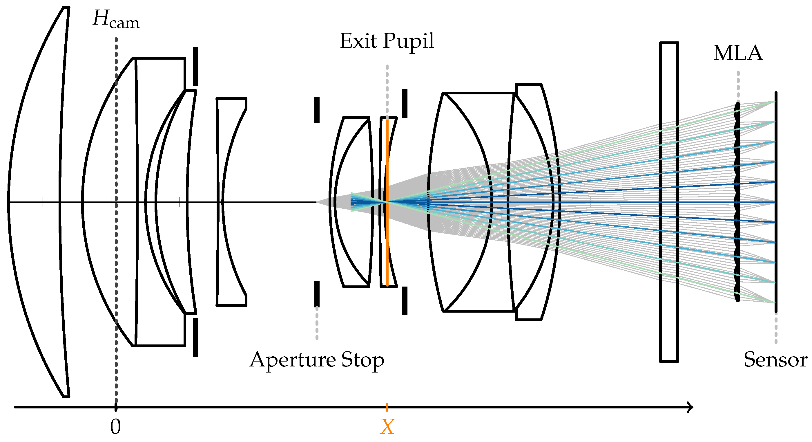
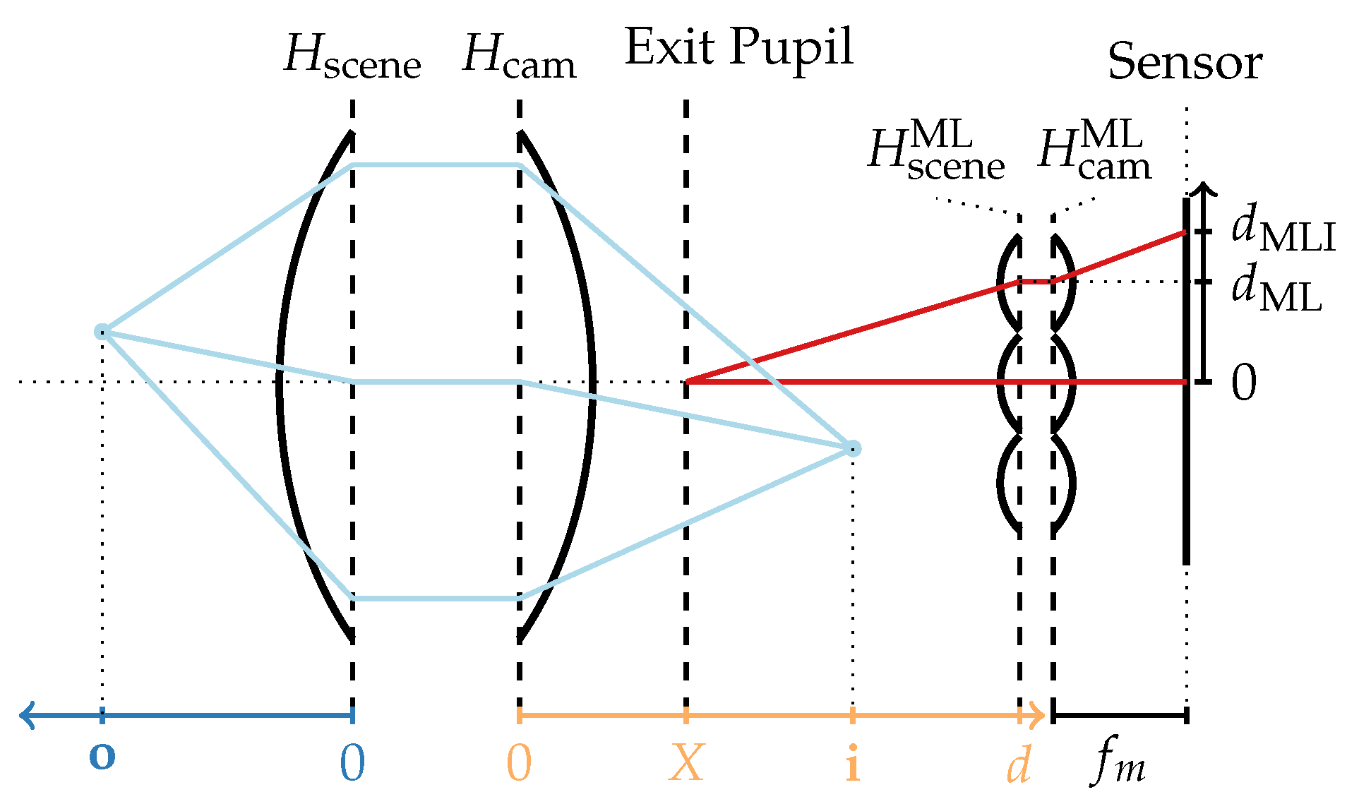
2. SPC Optics
2.1. Preliminaries—Lens Models
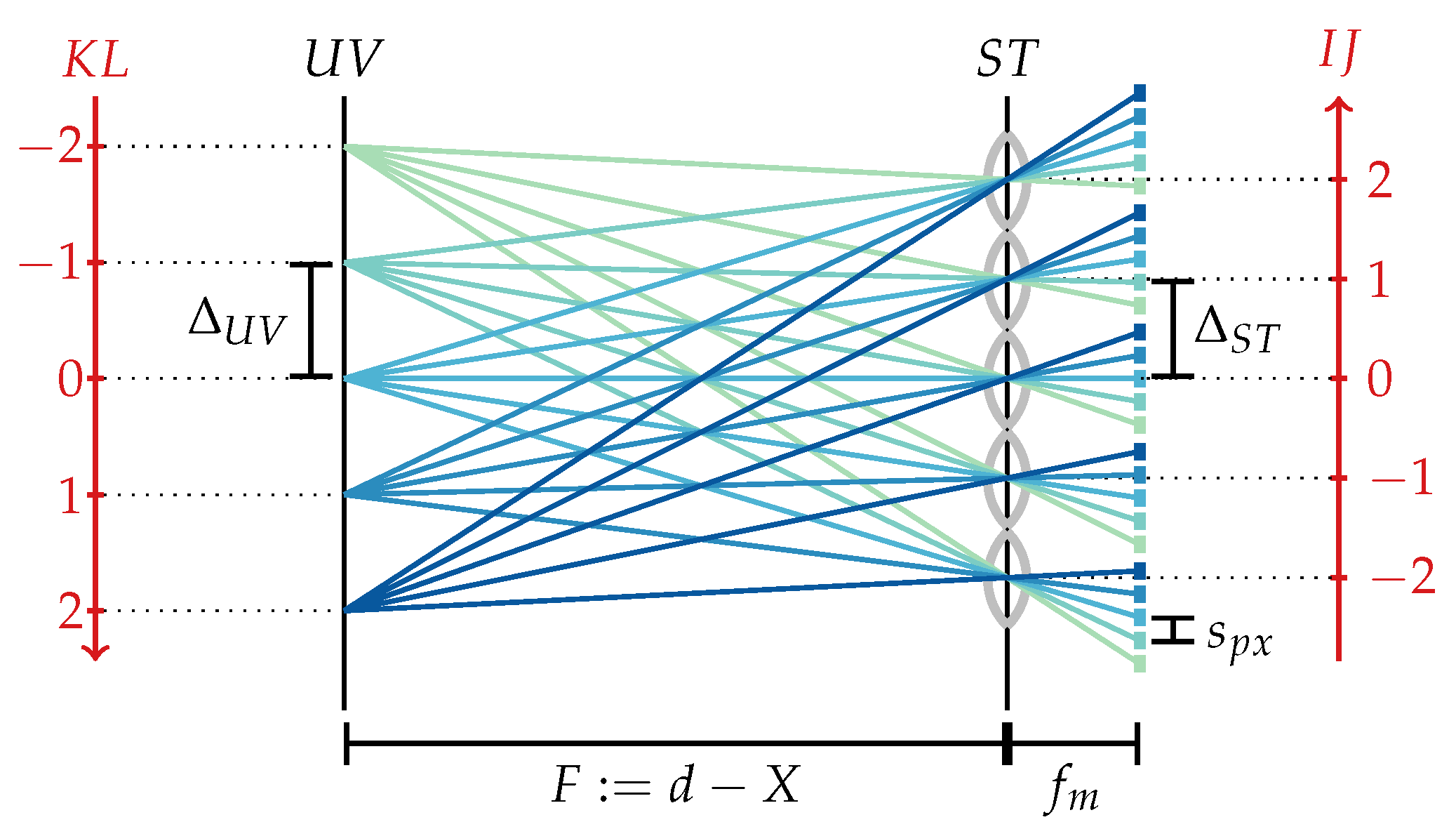
2.2. Preliminaries—Light Field Parametrization
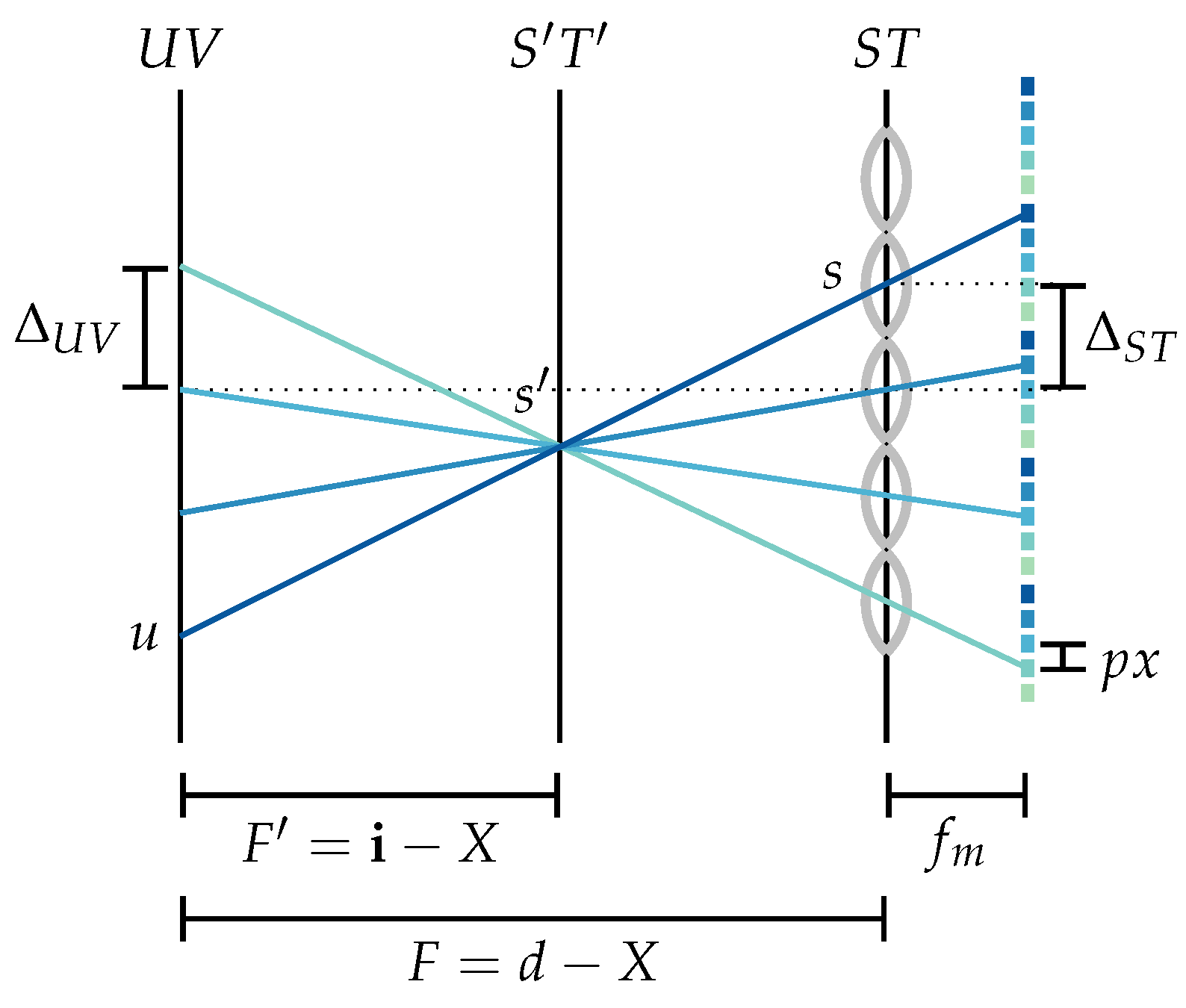
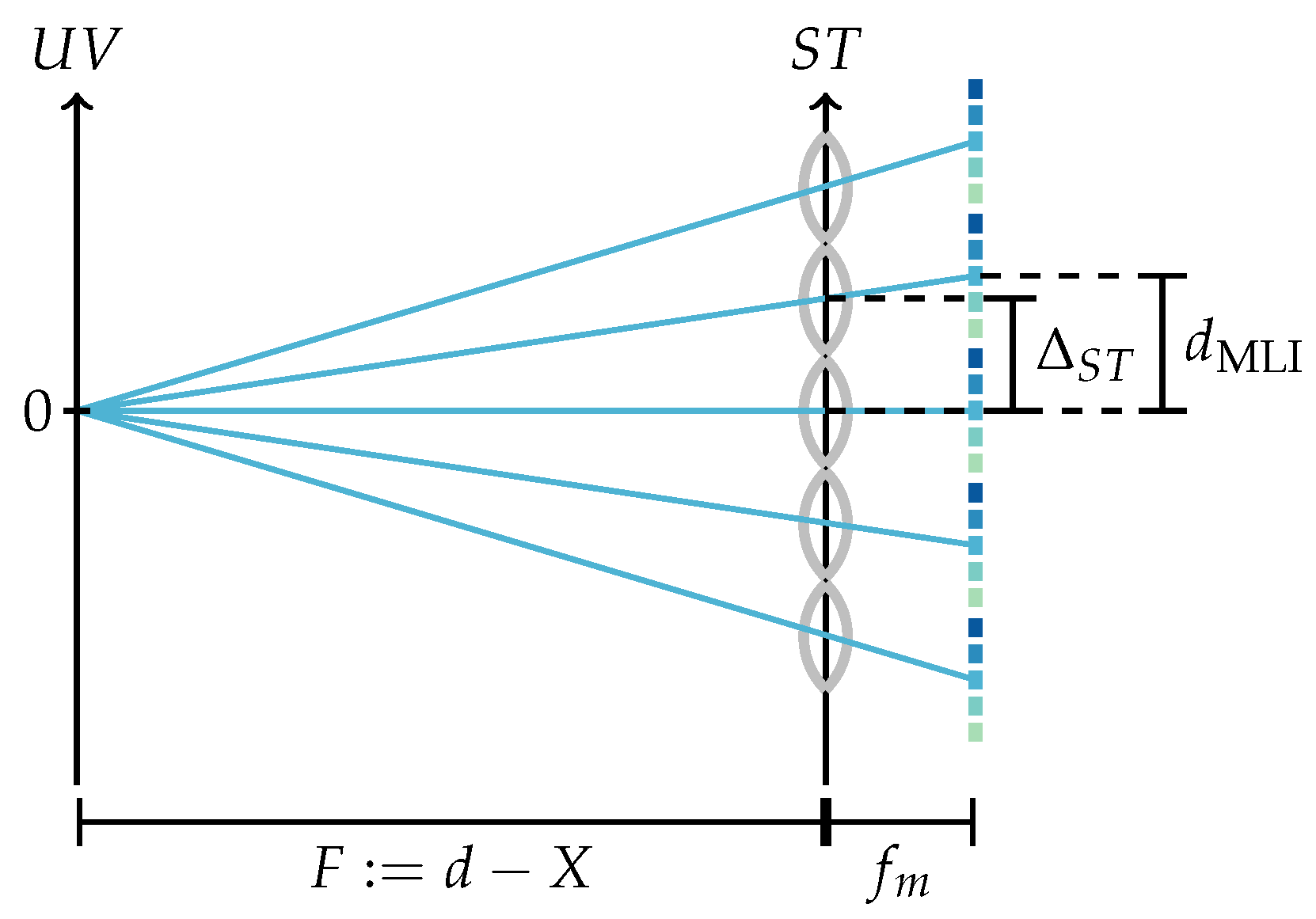
2.3. Light Field Refocusing with Exit Pupil
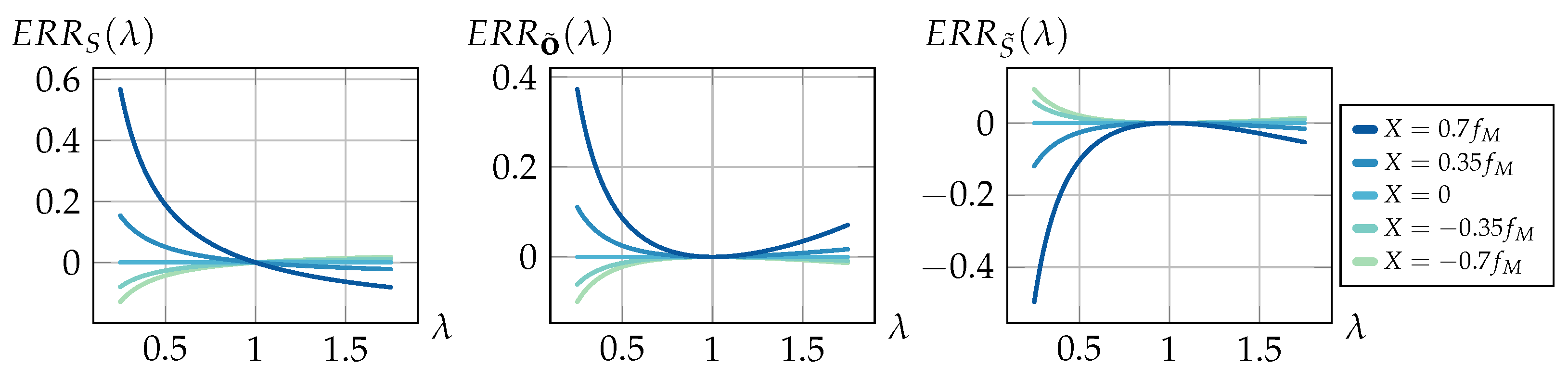
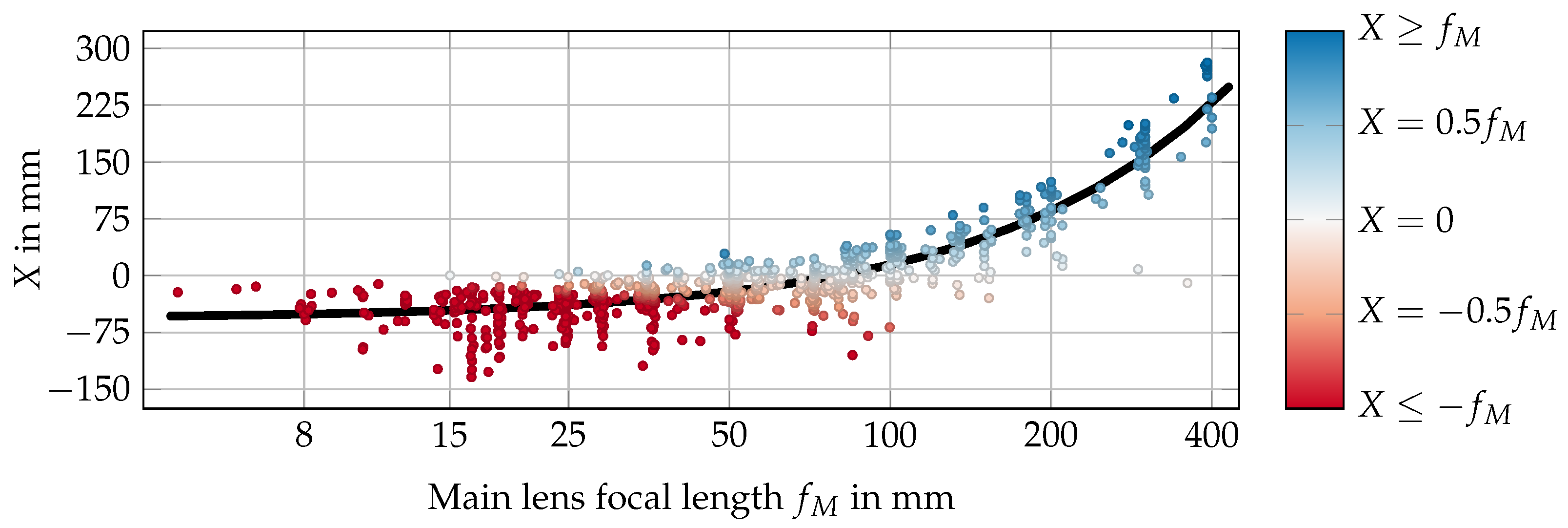
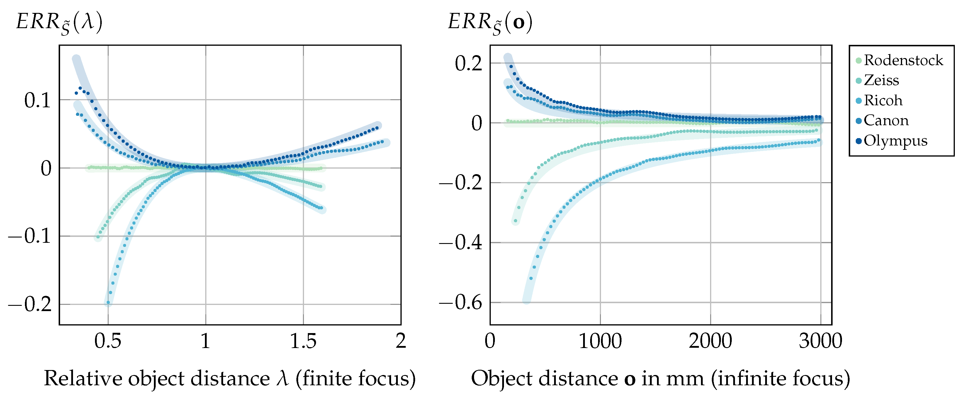
3. Error Analysis
4. Revisiting SPC Methods
4.1. Equivalent Ray Model
4.2. Light Field Decoding and SPC Calibration
4.3. Depth Reconstruction
5. Evaluation
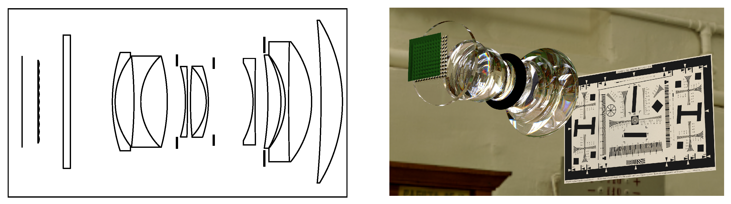
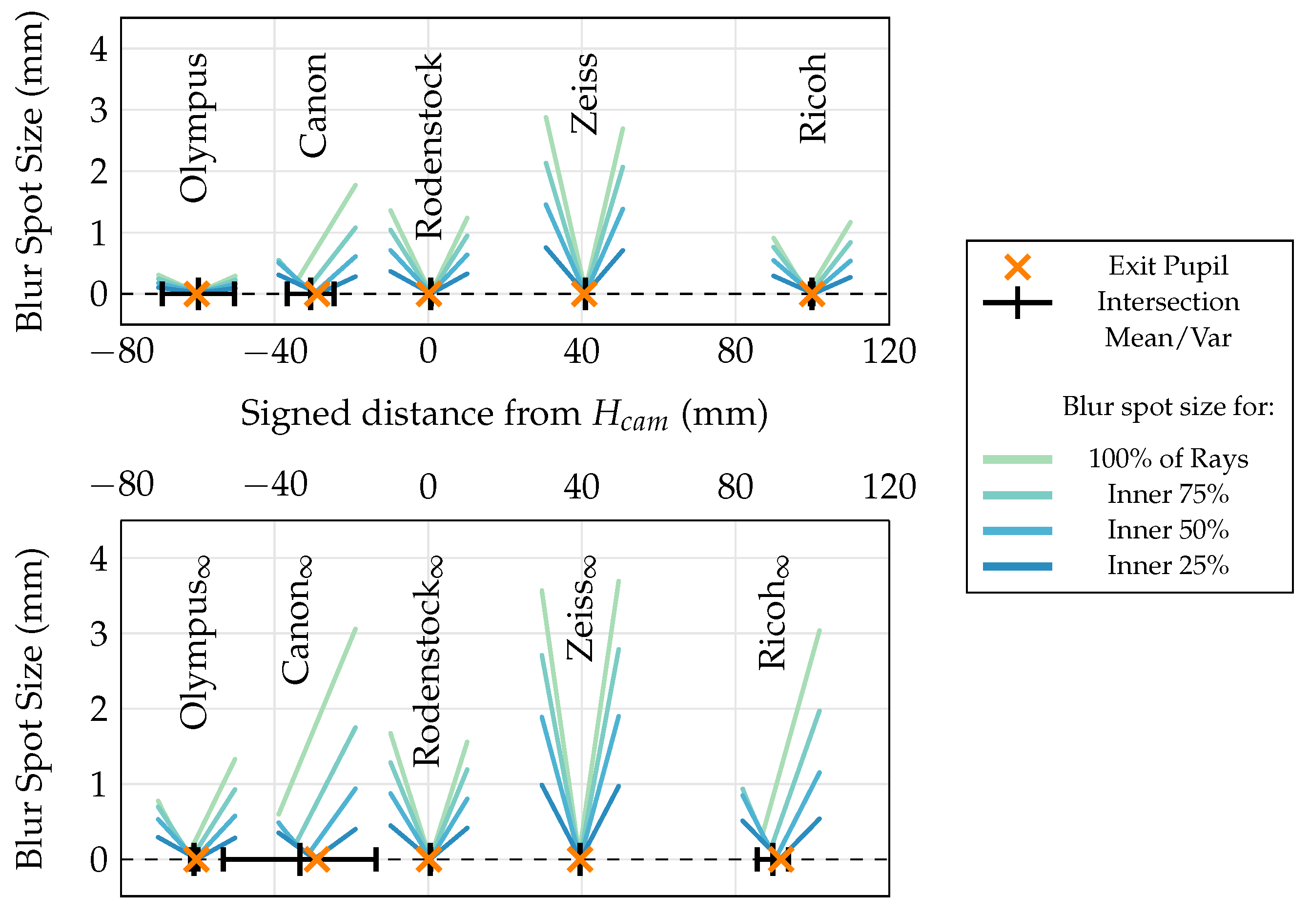
5.1. Simulation Environment
- Simulation of aspherical lenses and zoom lenses.
- Configurable MLA pose, thickness, and IOR.
- Automatic focusing with lens group movement based on paraxial approximations.
- Integration of Claff’s lens collection [47] and a collection of sensor presets.
- Assisted plenoptic camera (SPC and FPC) configuration based on the ideas of [48].
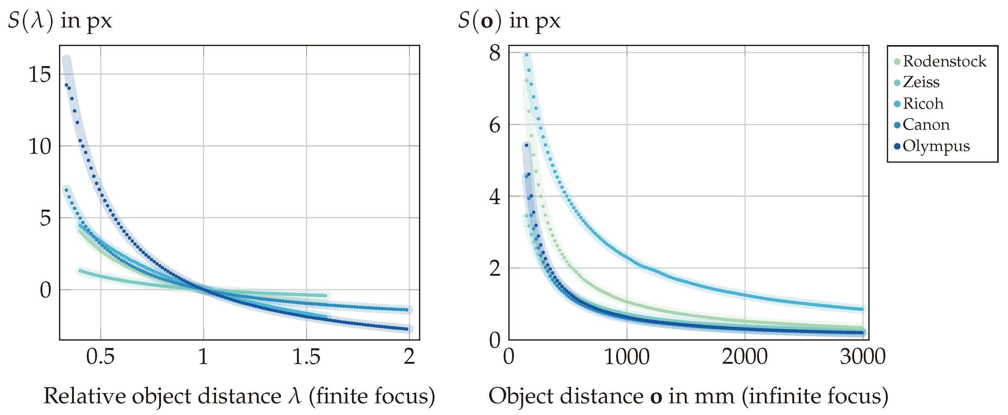
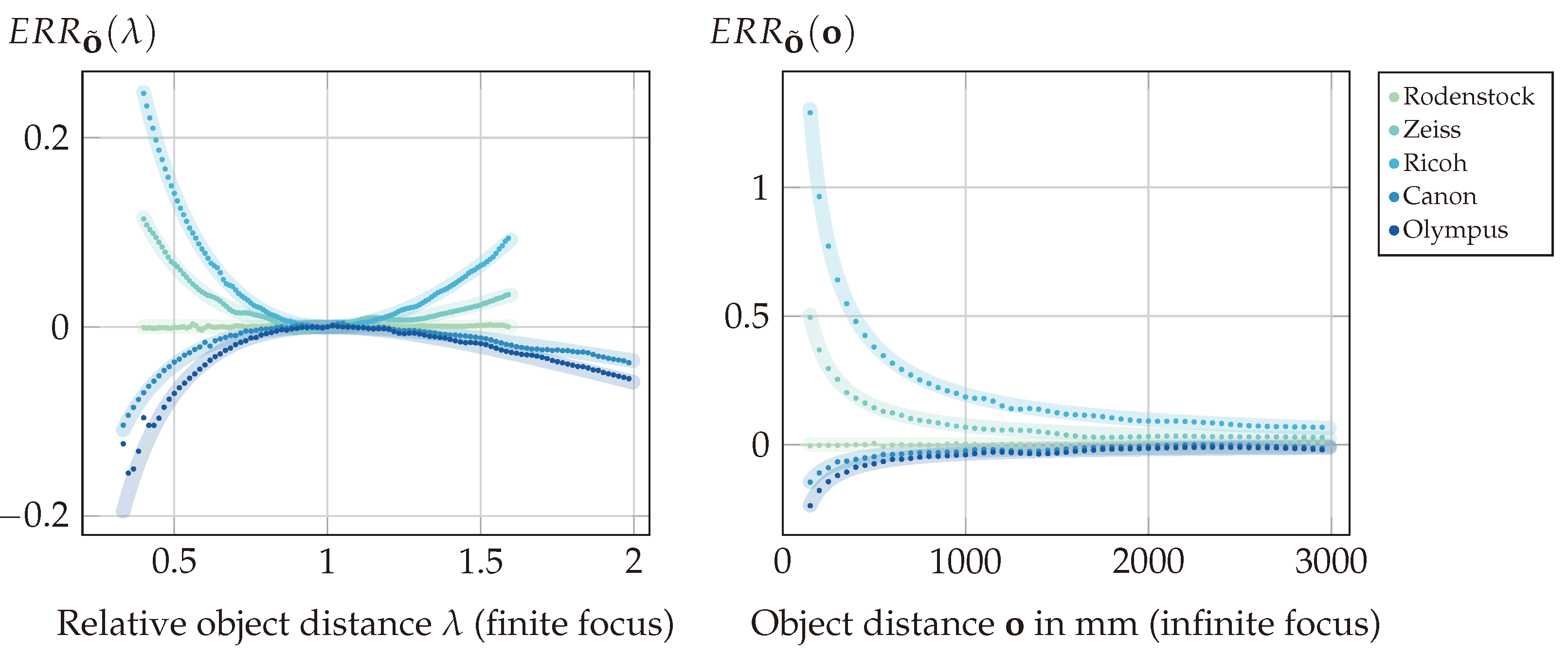
5.2. Experiments
5.3. Results and Discussion
6. Conclusion and Limitations
Author Contributions
Funding
Institutional Review Board Statement
Informed Consent Statement
Data Availability Statement
Acknowledgments
Conflicts of Interest
Abbreviations
| FPC | Focused Plenoptic Camera |
| MI | Microlens Image |
| MIC | Microlens Image Center |
| ML | Microlens |
| MLA | Microlens Array |
| SPC | Standard Plenoptic Camera |
Appendix A. Notation

| Parameter | Description |
|---|---|
| Main lens focal length | |
| Scene-side principal plane of the main lens | |
| Camera-side principal plane of the main lens | |
| X | Signed distance between and the exit pupil measured along the optical axis |
| Microlens focal length | |
| Scene-side principal plane of a microlens | |
| Camera-side principal plane of a microlens | |
| Object distance measured from | |
| Image distance measured from | |
| Focus distance | |
| d | Distance between the MLA’s and the main lens |
| Microlens pitch | |
| Pixel pitch, i.e., edge length of a square sensor pixel |
| Parameter | Description |
|---|---|
| F | Distance between and plane |
| Step size in the virtual lens plane | |
| Pixel pitch on the virtual sensor | |
| Scaling between the and step sizes, i.e., | |
| Integer indexed 4D light field | |
| Integer light field coordinates | |
| Metric parameterization of the 4D light field | |
| Metric light field coordinates |
| Parameter | Description |
|---|---|
| Distance between and plane for refocusing | |
| Refocusing parameter defined by | |
| , but for plane | |
| S | Sub-aperture image shift in pixels |
| S for a given refocusing distance | |
| Refocusing distance for a given shift S | |
| Quotient based on the assumption | |
| Sub-aperture image shift in pixels based on the assumption | |
| Refocusing distance based on the assumption | |
| Quotient | |
| Relative refocusing distance error for incorrect target distance model | |
| Relative refocusing distance error for incorrect shift model |
Appendix B. Revisited Literature—Notation Transfer
Appendix B.1. Hahne et al. [9]
| Description | Hahne et al. [9] | Our |
|---|---|---|
| Main lens focal length | ||
| Distance to MLA | d | |
| Distance to virtual image | ||
| Distance to scene object | ||
| Distance MLA to exit pupil | ||
| Distance MLA to virtual image | ||
| ML focal length | ||
| ML diameter | ||
| Pixel size |
| Description | Hahne et al. [9] |
|---|---|
| Horizontal number of microlenses | J |
| Microlens index | j |
| Microlens center of lens j | |
| Microlens image center of lens j | |
| Position of i-th neighbor pixel of MIC | |
| Slope of ray from i-th neighbor through ML center |
Appendix B.2. Dansereau et al. [7]
Appendix B.3. Pertuz et al. [10]
| Description | Pertuz et al. [10] | Our |
|---|---|---|
| Main lens focal length | f | |
| Focus distance (measured from ) | ||
| Corresponding image distance (equals distance MLA to ) | d | |
| Target distance | z | |
| Corresponding image distance | x | |
| Distance MLA to sensor (equals ML focal length) | ||
| ML diameter | D | |
| Pixel size | ||
| Separation between real and synthetic focal plane | ||
| Refocusing parameter (sub-aperture image shift) | ||
| UV plane step size |
Appendix C. Thick Microlenses

Appendix D. Evaluation Setups
| Manufacturer | Model | Patent |
|---|---|---|
| Rodenstock | Sironar-N 100 mm F5.6 | DE 2729831 Example 1 |
| Zeiss | Batis 85 mm F1.8 | JP 2015-096915 Example 2 |
| Ricoh | smc Pentax-A 200 mm F4 Macro ED | US 4,666,260 Example 1 |
| Canon | EF 85 mm F1.8 USM | JP 1993-157964 Example 1 |
| Olympus | Zuiko Auto-Zoom 85–250 mm F5 | US 4,025,167 Example 2 |
| Finite Focus | |||||
|---|---|---|---|---|---|
| Property | Rodenstock | Zeiss | Ricoh | Canon | Olympus |
| Focal Length (mm) | 99.998 | 82.047 | 167.994 | 84.998 | 85.120 |
| (mm) | −1.395 | −30.395 | −118.018 | −2.303 | 54.527 |
| (mm) | −0.981 | 36.192 | 83.127 | −27.317 | 1.026 |
| Exit Pupil Loc. (mm) | −1.201 | 10.257 | −18.109 | −31.241 | −5.690 |
| Exit Pupil Radius (mm) | 8.617 | 2.423 | 3.822 | 6.512 | 2.917 |
| X (mm) | 0.194 | 40.652 | 99.909 | −28.938 | −60.219 |
| f-number | 5.600 | 8.500 | 8.000 | 7.330 | 6.590 |
| Focus Distance F (mm) | 500 | 500 | 500 | 300 | 300 |
| ML Pitch (m) | 178.158 | 173.703 | 176.246 | 177.856 | 110.567 |
| ML Diam (m) | 178.158 | 173.703 | 176.285 | 177.856 | 110.567 |
| ML Focal Length (mm) | 1.290 | 2.084 | 3.261 | 1.779 | 0.884 |
| MLA Thickness (mm) | 0.100 | 0.100 | 0.100 | 0.100 | 0.100 |
| MLA-Sensor Dist (mm) | 1.280 | 2.084 | 3.261 | 1.779 | 0.874 |
| Aperture-Sensor Dist (mm) | 124.702 | 69.944 | 138.341 | 118.176 | 174.140 |
| Sensor Width (mm) | 23.220 | 23.220 | 23.220 | 23.220 | 7.222 |
| Sensor Height (mm) | 23.220 | 23.220 | 23.220 | 23.220 | 7.222 |
| Infinite Focus | |||||
|---|---|---|---|---|---|
| Property | Rodenstock | Zeiss | Ricoh | Canon | Olympus |
| Focal Length (mm) | 99.998 | 82.860 | 173.115 | 84.998 | 85.004 |
| (mm) | −1.395 | −29.315 | −109.963 | −2.303 | 54.617 |
| (mm) | −0.981 | 34.023 | 75.005 | −27.317 | 1.155 |
| Exit Pupil Loc. (mm) | −1.201 | 10.257 | −18.109 | −31.241 | −5.690 |
| Exit Pupil Radius (mm) | 8.617 | 3.817 | 7.093 | 6.512 | 9.290 |
| X (mm) | 0.194 | 39.572 | 91.525 | −28.938 | −60.308 |
| f-number | 5.600 | 5.870 | 9.100 | 8.000 | 7.660 |
| Focus Distance F (mm) | ∞ | ∞ | ∞ | ∞ | ∞ |
| ML Pitch (m) | 178.158 | 175.944 | 177.164 | 177.840 | 171.492 |
| ML Diam (m) | 178.158 | 175.944 | 177.164 | 177.840 | 171.492 |
| ML Focal Length (mm) | 1.032 | 0.998 | 1.230 | 1.383 | 1.297 |
| MLA Thickness (mm) | 0.100 | 0.100 | 0.100 | 0.100 | 0.100 |
| MLA-Sensor Dist (mm) | 1.022 | 0.987 | 1.220 | 1.373 | 1.287 |
| Aperture-Sensor Dist (mm) | 99.745 | 54.659 | 64.521 | 84.189 | 141.035 |
| Sensor Width (mm) | 23.220 | 23.220 | 23.200 | 23.220 | 22.32 |
| Sensor Height (mm) | 23.220 | 23.220 | 23.200 | 23.220 | 22.32 |
References
- Lippmann, G. La photographie integrale. Comptes-Rendus 1908, 146, 446–451. [Google Scholar]
- Ives, H.E. A camera for making parallax panoramagrams. Josa 1928, 17, 435–439. [Google Scholar] [CrossRef]
- Adelson, E.H.; Wang, J.Y. Single lens stereo with a plenoptic camera. IEEE Trans. Pattern Anal. Mach. Intell. 1992, 14, 99–106. [Google Scholar] [CrossRef]
- Ng, R.; Levoy, M.; Brédif, M.; Duval, G.; Horowitz, M.; Hanrahan, P. Light Field Photography with a Hand-Held Plenoptic Camera. Ph.D. Thesis, Stanford University, Stanford, CA, USA, 2005. [Google Scholar]
- Georgiev, T.; Intwala, C. Light field camera design for integral view photography. In Technical Report; Adobe System, Inc.: San Jose, CA, USA, 2006; p. 1. [Google Scholar]
- Perwass, C.; Wietzke, L. Single lens 3D-camera with extended depth-of-field. In Proceedings of the Human Vision and Electronic Imaging XVII, SPIE, Burlingame, CA, USA, 22 January 2012; Volume 8291, pp. 45–59. [Google Scholar]
- Dansereau, D.G.; Pizarro, O.; Williams, S.B. Decoding, calibration and rectification for lenselet-based plenoptic cameras. In Proceedings of the 2013 IEEE Conference on Computer Vision and Pattern Recognition (CVPR), Portland, OR, USA, 23–28 June 2013; pp. 1027–1034. [Google Scholar]
- Hahne, C.; Aggoun, A.; Velisavljevic, V.; Fiebig, S.; Pesch, M. Baseline and triangulation geometry in a standard plenoptic camera. Int. J. Comput. Vis. 2018, 126, 21–35. [Google Scholar] [CrossRef]
- Hahne, C.; Aggoun, A.; Velisavljevic, V.; Fiebig, S.; Pesch, M. Refocusing distance of a standard plenoptic camera. Opt. Express 2016, 24, 21521–21540. [Google Scholar] [CrossRef]
- Pertuz, S.; Pulido-Herrera, E.; Kamarainen, J.K. Focus model for metric depth estimation in standard plenoptic cameras. ISPRS J. Photogramm. Remote Sens. 2018, 144, 38–47. [Google Scholar] [CrossRef]
- Blender Foundation. Available online: https://www.blender.org/ (accessed on 12 January 2024).
- Zhang, Q.; Zhang, C.; Ling, J.; Wang, Q.; Yu, J. A generic multi-projection-center model and calibration method for light field cameras. IEEE Trans. Pattern Anal. Mach. Intell. 2018, 41, 2539–2552. [Google Scholar] [CrossRef]
- Monteiro, N.B.; Barreto, J.P.; Gaspar, J.A. Standard plenoptic cameras mapping to camera arrays and calibration based on DLT. IEEE Trans. Circuits Syst. Video Technol. 2019, 30, 4090–4099. [Google Scholar] [CrossRef]
- Van Duong, V.; Canh, T.N.; Huu, T.N.; Jeon, B. Focal stack based light field coding for refocusing applications. In Proceedings of the 2019 IEEE International Symposium on Broadband Multimedia Systems and Broadcasting (BMSB), Jeju, Republic of Korea, 5–7 June 2019; pp. 1–4. [Google Scholar]
- Michels, T. SPC Designs. Available online: https://gitlab.com/ungetym/SPC-revisited (accessed on 22 February 2024).
- Michels, T. Blender Camera Generator Add-On. Available online: https://gitlab.com/ungetym/blender-camera-generator (accessed on 22 February 2024).
- Lumsdaine, A.; Georgiev, T. The focused plenoptic camera. In Proceedings of the 2009 IEEE International Conference on Computational Photography (ICCP), San Francisco, CA, USA, 16–17 April 2009; pp. 1–8. [Google Scholar]
- Wanner, S.; Goldluecke, B. Globally consistent depth labeling of 4D light fields. In Proceedings of the 2012 IEEE Conference on Computer Vision and Pattern Recognition, Providence, RI, USA, 16–21 June 2012; pp. 41–48. [Google Scholar]
- Georgiev, T.; Lumsdaine, A. Focused plenoptic camera and rendering. J. Electron. Imaging 2010, 19, 021106. [Google Scholar]
- Bok, Y.; Jeon, H.G.; Kweon, I.S. Geometric calibration of micro-lens-based light field cameras using line features. IEEE Trans. Pattern Anal. Mach. Intell. 2016, 39, 287–300. [Google Scholar] [CrossRef]
- Zhao, Y.; Li, H.; Mei, D.; Shi, S. Metric calibration of unfocused plenoptic cameras for three-dimensional shape measurement. Opt. Eng. 2020, 59, 073104. [Google Scholar] [CrossRef]
- Thomason, C.M.; Thurow, B.S.; Fahringer, T.W. Calibration of a microlens array for a plenoptic camera. In Proceedings of the 52nd Aerospace Sciences Meeting, National Harbor, MD, USA, 13–17 January 2014; p. 396. [Google Scholar]
- Suliga, P.; Wrona, T. Microlens array calibration method for a light field camera. In Proceedings of the 2018 19th International Carpathian Control Conference (ICCC), Szilvasvarad, Hungary, 28–31 May 2018; pp. 19–22. [Google Scholar]
- Schambach, M.; León, F.P. Microlens array grid estimation, light field decoding, and calibration. IEEE Trans. Comput. Imaging 2020, 6, 591–603. [Google Scholar] [CrossRef]
- Mignard-Debise, L.; Ihrke, I. A vignetting model for light field cameras with an application to light field microscopy. IEEE Trans. Comput. Imaging 2019, 5, 585–595. [Google Scholar] [CrossRef]
- Johannsen, O.; Heinze, C.; Goldluecke, B.; Perwaß, C. On the calibration of focused plenoptic cameras. In Time-of-Flight and Depth Imaging. Sensors, Algorithms, and Applications: Dagstuhl 2012 Seminar on Time-of-Flight Imaging and GCPR 2013 Workshop on Imaging New Modalities; Springer: Berlin/Heidelberg, Germany, 2013; pp. 302–317. [Google Scholar]
- Heinze, C.; Spyropoulos, S.; Hussmann, S.; Perwaß, C. Automated robust metric calibration algorithm for multifocus plenoptic cameras. IEEE Trans. Instrum. Meas. 2016, 65, 1197–1205. [Google Scholar] [CrossRef]
- Zeller, N.; Noury, C.; Quint, F.; Teulière, C.; Stilla, U.; Dhome, M. Metric calibration of a focused plenoptic camera based on a 3D calibration target. ISPRS Ann. Photogramm. Remote Sens. Spat. Inf. Sci. 2016, 3, 449–456. [Google Scholar] [CrossRef]
- Noury, C.A.; Teulière, C.; Dhome, M. Light-field camera calibration from raw images. In Proceedings of the 2017 International Conference on Digital Image Computing: Techniques and Applications (DICTA), Sydney, Australia, 29 November–1 December 2017; pp. 1–8. [Google Scholar]
- Nousias, S.; Chadebecq, F.; Pichat, J.; Keane, P.; Ourselin, S.; Bergeles, C. Corner-based geometric calibration of multi-focus plenoptic cameras. In Proceedings of the IEEE International Conference on Computer Vision, Venice, Italy, 22–29 October 2017; pp. 957–965. [Google Scholar]
- Wang, Y.; Qiu, J.; Liu, C.; He, D.; Kang, X.; Li, J.; Shi, L. Virtual image points based geometrical parameters’ calibration for focused light field camera. IEEE Access 2018, 6, 71317–71326. [Google Scholar] [CrossRef]
- Labussière, M.; Teulière, C.; Bernardin, F.; Ait-Aider, O. Leveraging blur information for plenoptic camera calibration. Int. J. Comput. Vis. 2022, 130, 1655–1677. [Google Scholar] [CrossRef]
- Kolb, C.; Mitchell, D.; Hanrahan, P. A realistic camera model for computer graphics. In Proceedings of the 22nd Annual Conference on Computer Graphics and Interactive Techniques, Los Angeles, CA, USA, 6–11 August 1995; pp. 317–324. [Google Scholar]
- Wu, J.; Zheng, C.; Hu, X.; Li, C. An accurate and practical camera lens model for rendering realistic lens effects. In Proceedings of the 2011 12th International Conference on Computer-Aided Design and Computer Graphics, Jinan, China, 15–17 September 2011; pp. 63–70. [Google Scholar]
- Zheng, Q.; Zheng, C. NeuroLens: Data-Driven Camera Lens Simulation Using Neural Networks. In Proceedings of the Computer Graphics Forum, Wiley Online Library, Lyon, France, 24–26 April 2017; Volume 36, pp. 390–401. [Google Scholar]
- Fleischmann, O.; Koch, R. Lens-based depth estimation for multi-focus plenoptic cameras. In Proceedings of the German Conference on Pattern Recognition. Springer, Münster, Germany, 2–5 September 2014; pp. 410–420. [Google Scholar]
- Zhang, R.; Liu, P.; Liu, D.; Su, G. Reconstruction of refocusing and all-in-focus images based on forward simulation model of plenoptic camera. Opt. Commun. 2015, 357, 1–6. [Google Scholar] [CrossRef]
- Liang, C.K.; Ramamoorthi, R. A light transport framework for lenslet light field cameras. ACM Trans. Graph. (TOG) 2015, 34, 16. [Google Scholar] [CrossRef]
- Nürnberg, T.; Schambach, M.; Uhlig, D.; Heizmann, M.; León, F.P. A simulation framework for the design and evaluation of computational cameras. In Proceedings of the Automated Visual Inspection and Machine Vision III, International Society for Optics and Photonics, Munich, Germany, 24–27 June 2019; Volume 11061, p. 1106102. [Google Scholar]
- Michels, T.; Petersen, A.; Palmieri, L.; Koch, R. Simulation of plenoptic cameras. In Proceedings of the 2018-3DTV-Conference: The True Vision-Capture, Transmission and Display of 3D Video (3DTV-CON), Helsinki, Finland, 3–5 June 2018; pp. 1–4. [Google Scholar]
- Born, M.; Wolf, E. Principles of Optics: Electromagnetic Theory of Propagation, Interference and Diffraction of Light; Elsevier: Amsterdam, The Netherlands, 2013. [Google Scholar]
- Smith, W.J. Modern Optical Engineering: The Design of Optical Systems; McGraw-Hill Education: New York, NY, USA, 2008. [Google Scholar]
- Levoy, M.; Hanrahan, P. Light field rendering. In Computer Graphics Proceedings, Annual Conference Series; Association for Computing Machinery SIGGRAPH: New Orleans, LA, USA, 1996; pp. 31–42. [Google Scholar]
- Ng, R. Fourier slice photography. In ACM Siggraph 2005 Papers; Association for Computing Machinery: New York, NY, USA, 2005; pp. 735–744. [Google Scholar]
- Carl Zeiss AG, Datasheet: Zeiss Planar T* 2/80 Lens Datasheet. Available online: https://www.zeiss.de/content/dam/consumer-products/downloads/historical-products/photography/contax-645/de/datasheet-zeiss-planar-280-de.pdf (accessed on 12 January 2024).
- Carl Zeiss AG, Datasheet: Zeiss Zeiss Sonnar T* 2.8/140. Available online: https://www.zeiss.de/content/dam/consumer-products/downloads/historical-products/photography/contax-645/de/datasheet-zeiss-sonnar-28140-de.pdf (accessed on 12 January 2024).
- Claff, W.J. Available online: https://www.photonstophotos.net (accessed on 12 January 2024).
- Michels, T.; Koch, R. Ray tracing-guided design of plenoptic cameras. In Proceedings of the 2021 International Conference on 3D Vision (3DV), London, UK, 1–3 December 2021; pp. 1125–1133. [Google Scholar]
- ISO 12233 Pattern, Cornell University. Available online: https://www.graphics.cornell.edu/~westin/misc/res-chart.html (accessed on 1 April 2024).
- Yu, W. Practical anti-vignetting methods for digital cameras. IEEE Trans. Consum. Electron. 2004, 50, 975–983. [Google Scholar]
- Pertuz, S.; Puig, D.; Garcia, M.A. Analysis of focus measure operators for shape-from-focus. Pattern Recognit. 2013, 46, 1415–1432. [Google Scholar] [CrossRef]
- Freniere, E.R.; Gregory, G.G.; Hassler, R.A. Edge diffraction in Monte Carlo ray tracing. In Proceedings of the Optical Design and Analysis Software, SPIE, Denver, CO, USA, 21–22 July 1999; Volume 3780, pp. 151–157. [Google Scholar]
- Mahan, J.; Vinh, N.; Ho, V.; Munir, N. Monte Carlo ray-trace diffraction based on the Huygens–Fresnel principle. Appl. Opt. 2018, 57, D56–D62. [Google Scholar] [CrossRef] [PubMed]


| Finite Focus | Infinite Focus | ||||||
|---|---|---|---|---|---|---|---|
| Lens Model | (mm) | (mm) |
Focus
Dist. (mm) | (mm) | (mm) | ||
| Rodenstock Sironar-N 100 mm F5.6 | 99.998 | 0.194 | 0.002 | 500.0 | 99.998 | 0.194 | 0.002 |
| Zeiss Batis 85 mm F1.8 | 82.047 | 40.652 | 0.496 | 500.0 | 82.860 | 39.573 | 0.478 |
| Ricoh smc Pentax-A 200 mm F4 Macro ED | 167.994 | 99.908 | 0.595 | 500.0 | 173.115 | 91.854 | 0.531 |
| Canon EF 85 mm F1.8 USM | 84.998 | −28.938 | −0.341 | 300.0 | 84.998 | −28.938 | −0.341 |
| Olympus Zuiko Auto-Zoom 85–250 mm F5 | 85.120 | −60.219 | −0.708 | 300.0 | 85.004 | −60.308 | −0.709 |
| Pertuz et al. [10] | Ours (Equation (32)) | Fitted | |||||||
|---|---|---|---|---|---|---|---|---|---|
| Setup | RMSE | RMSE | RMSE | ||||||
| Rodens. | 0.0927 | 0.4633 | 21.03 | −0.00014 | 0.3705 | 0.64 | −0.00038 | 0.36951 | 0.49 |
| Zeiss | 0.1853 | 1.1294 | 28.05 | −0.13102 | 0.81304 | 1.51 | −0.13109 | 0.81361 | 1.51 |
| Ricoh | 0.1140 | 0.3391 | 89.77 | −0.07435 | 0.15079 | 0.52 | −0.07403 | 0.15111 | 0.51 |
| Canon | 0.1341 | 0.4733 | 45.50 | 0.02630 | 0.36553 | 0.74 | 0.025547 | 0.36568 | 0.59 |
| Olympus | 0.0674 | 0.2376 | 37.49 | 0.02267 | 0.19286 | 1.12 | 0.0213 | 0.19146 | 0.62 |
| Rodens.∞ | 0.0927 | 55.588 | 96.87 | −0.00018 | 55.495 | 7.19 | 0.00198 | 55.625 | 6.83 |
| Zeiss∞ | 0.1070 | 322.73 | 153.30 | −0.09773 | 322.53 | 9.67 | −0.08574 | 323.61 | 8.35 |
| Ricoh∞ | 0.0635 | 366.78 | 364.78 | −0.07175 | 366.65 | 6.76 | −0.06887 | 367.54 | 5.03 |
| Canon∞ | 0.1458 | 1715.1 | 67.40 | 0.03702 | 1715 | 10.26 | 0.04576 | 1724.1 | 8.69 |
| Olympus∞ | 0.1370 | 96.683 | 46.52 | 0.05680 | 96.603 | 8.23 | 0.06014 | 96.631 | 8.07 |
Disclaimer/Publisher’s Note: The statements, opinions and data contained in all publications are solely those of the individual author(s) and contributor(s) and not of MDPI and/or the editor(s). MDPI and/or the editor(s) disclaim responsibility for any injury to people or property resulting from any ideas, methods, instructions or products referred to in the content. |
© 2024 by the authors. Licensee MDPI, Basel, Switzerland. This article is an open access article distributed under the terms and conditions of the Creative Commons Attribution (CC BY) license (https://creativecommons.org/licenses/by/4.0/).
Share and Cite
Michels, T.; Mäckelmann, D.; Koch, R. Mind the Exit Pupil Gap: Revisiting the Intrinsics of a Standard Plenoptic Camera. Sensors 2024, 24, 2522. https://doi.org/10.3390/s24082522
Michels T, Mäckelmann D, Koch R. Mind the Exit Pupil Gap: Revisiting the Intrinsics of a Standard Plenoptic Camera. Sensors. 2024; 24(8):2522. https://doi.org/10.3390/s24082522
Chicago/Turabian StyleMichels, Tim, Daniel Mäckelmann, and Reinhard Koch. 2024. "Mind the Exit Pupil Gap: Revisiting the Intrinsics of a Standard Plenoptic Camera" Sensors 24, no. 8: 2522. https://doi.org/10.3390/s24082522
APA StyleMichels, T., Mäckelmann, D., & Koch, R. (2024). Mind the Exit Pupil Gap: Revisiting the Intrinsics of a Standard Plenoptic Camera. Sensors, 24(8), 2522. https://doi.org/10.3390/s24082522