
Reconstruction of Radio Environment Map Based on Multi-Source Domain Adaptive of Graph Neural Network for Regression

Abstract
1. Introduction
- (1)
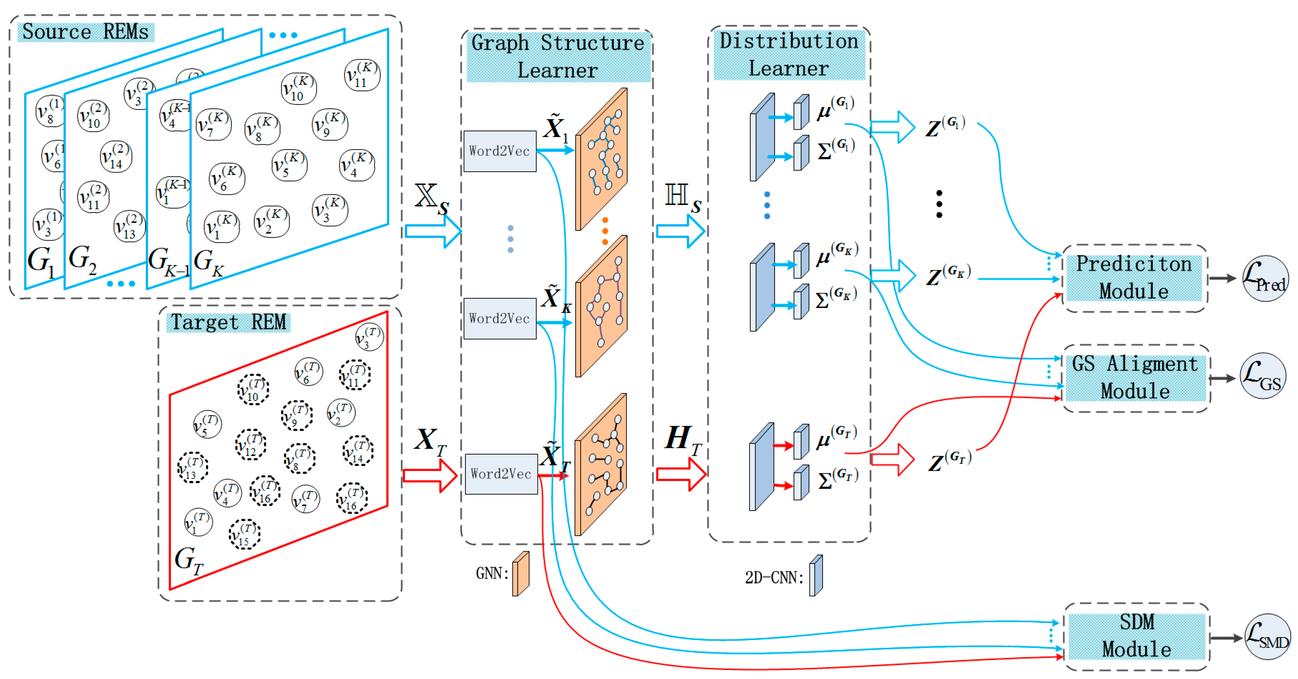
- Introducing multiple different spatial REMs to enhance training data also leads to cross-domain drift issues in graph structure data statistical characteristics. To address this, we introduce the idea of variational graph structure learning into multi-domain adaptation algorithms and design a cross-domain graph structure (GS) alignment module based on the theory of variational information bottleneck. This module is used to learn the spatial graph structure shared information of grid features in source and target REMs.
- (2)
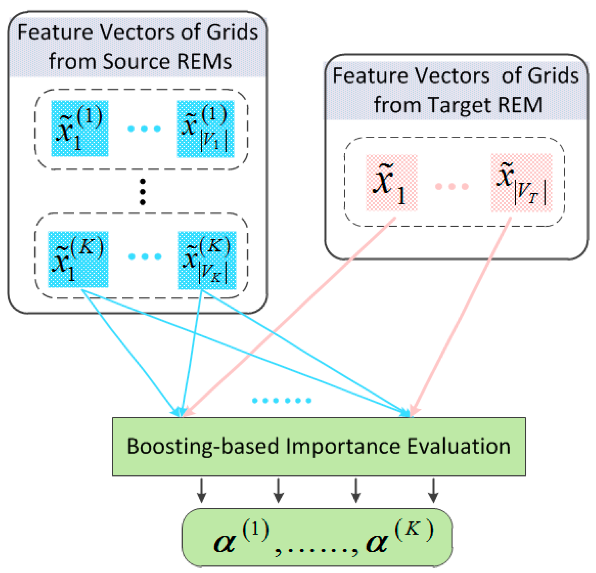
- In the process of multi-source domain adaptation learning, to avoid the problem of suppressing target domain task performance caused by the forced migration of low-correlation grid features from the source domain, we also designed a spatial distribution matching module. This module achieves alignment of source and target domain grid features in the latent space, capturing the domain invariance of cross-domain REM grids. It enhances the generalization capability of the proposed model for predicting RSRP values in target REM grids.
- (3)
- We constructed a semi-supervised learning loss function related to the multi-domain adaptive (MDA) REM prediction task. Specifically, we used grid data with RSRP values from source and target REMs to construct the supervised loss function, ensuring the consistency of the trained model with the given label data. We also used grid data without RSRP values from the target REM to construct a semi-supervised loss function to force the regression model to smoothly fit the RSRP prediction data.
2. Related Works
2.1. Distribution Matching
2.2. Domain Adaptation for Regression
3. Preliminaries
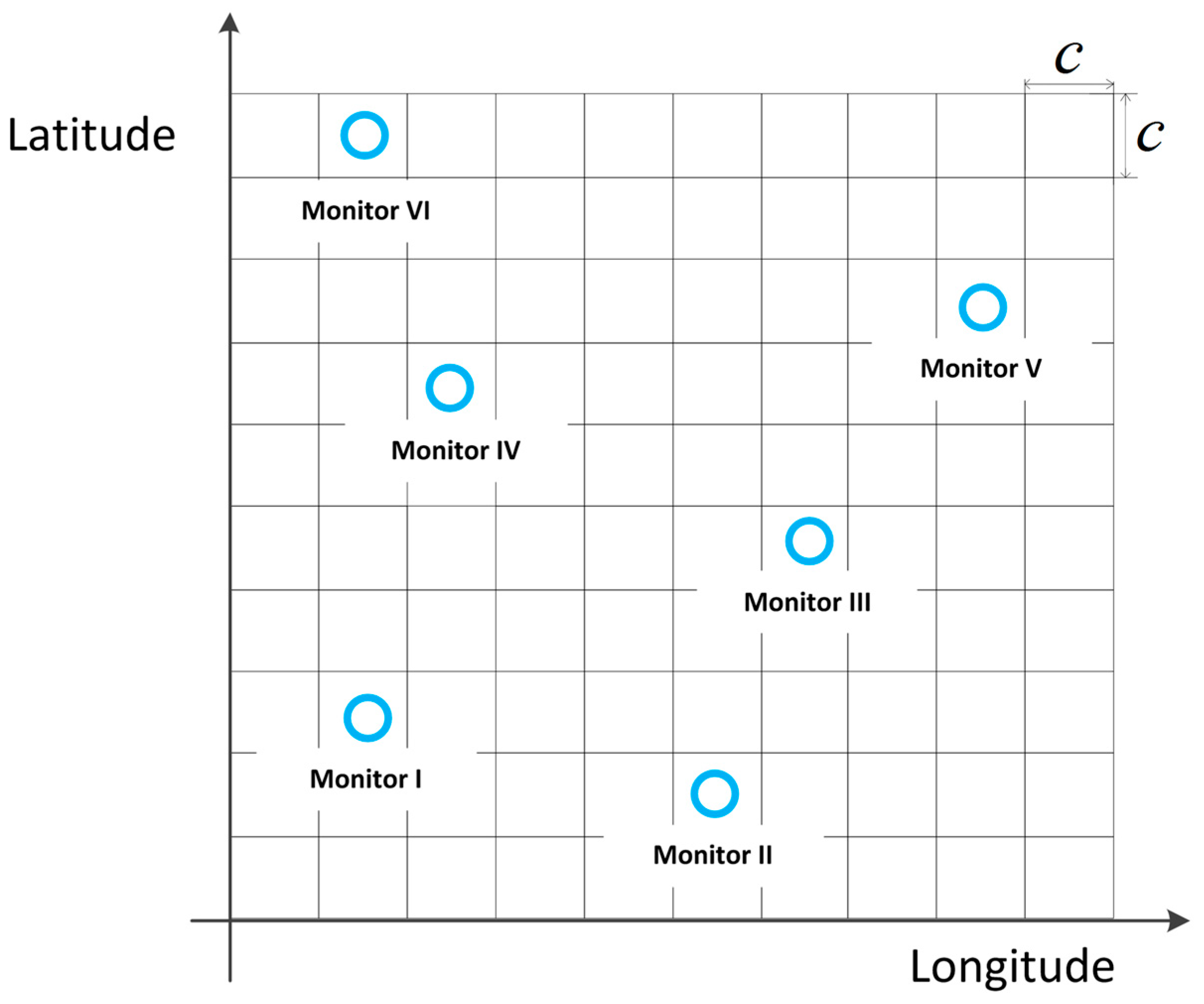
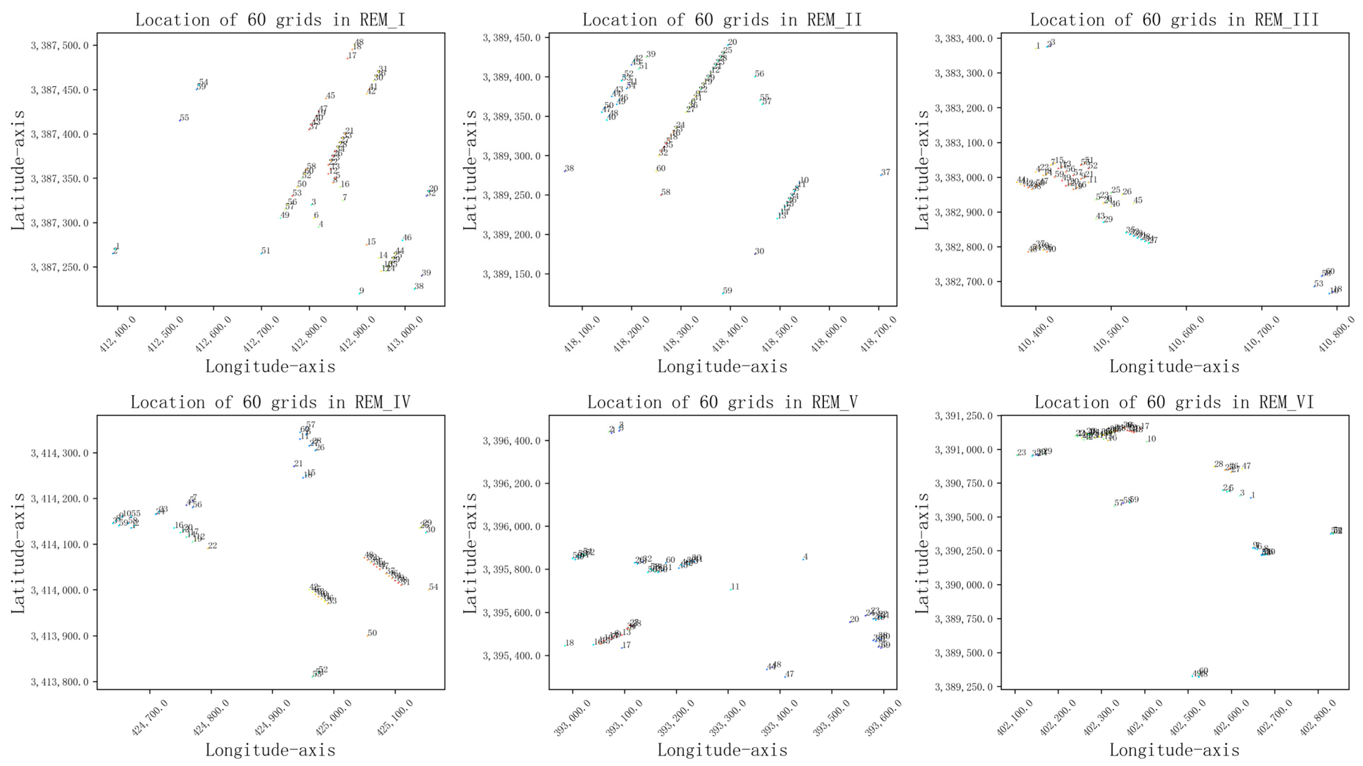
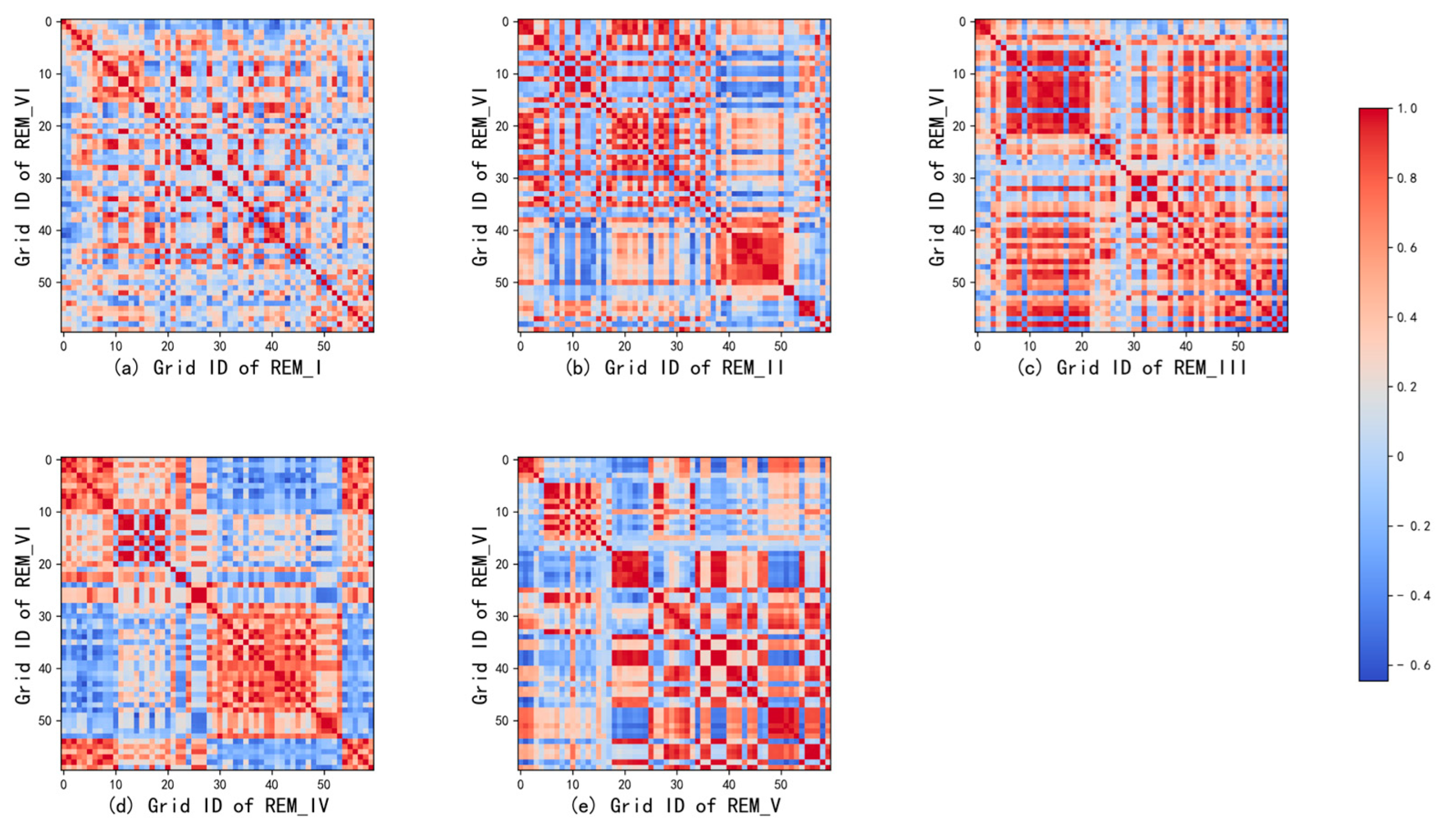
3.1. Graph Structure Representation for REM
3.2. Graph Neural Networks
3.3. Problem Definition
4. Methods
4.1. Graph Structure Learner
4.2. Distribution Learner of Latent Feature
4.3. Graph Structure Alignment
4.4. Spatial Distribution Matching
4.5. Loss Function for Regression
4.6. Overall Loss Function
5. Experiments
5.1. Experiment Setup
5.2. Experimental Results and Analysis
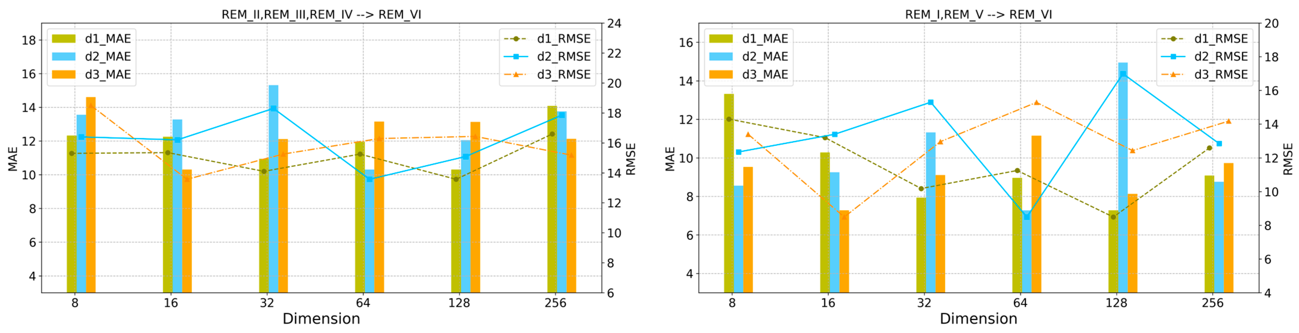
5.2.1. Discussion on the Output Dimensions of Each Network Layer
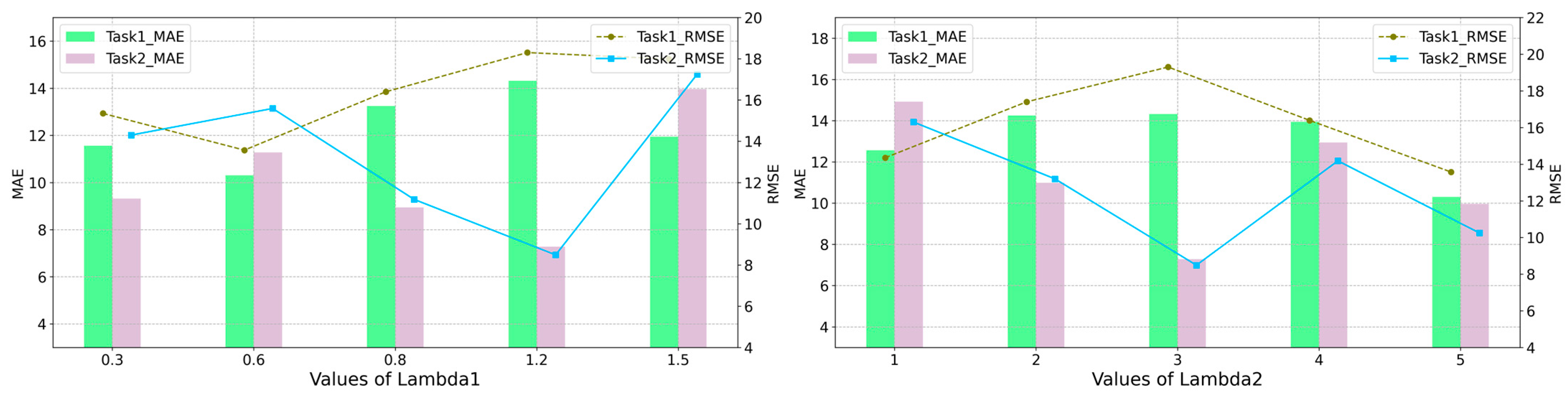
5.2.2. Discussion on the Effect of Trade-Off Parameters
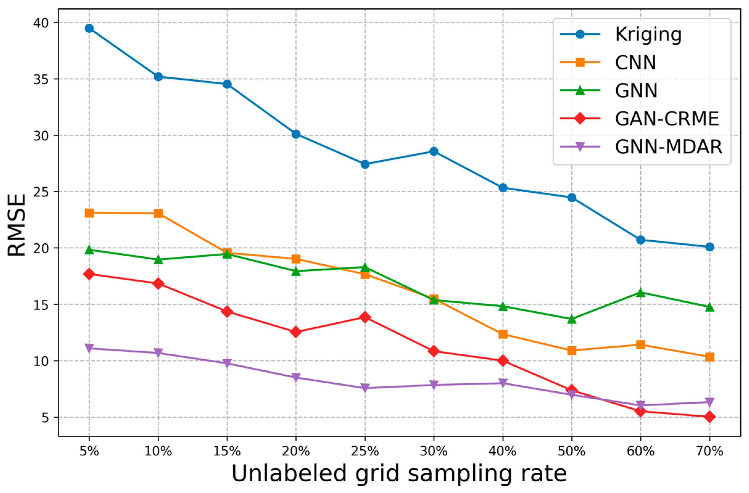
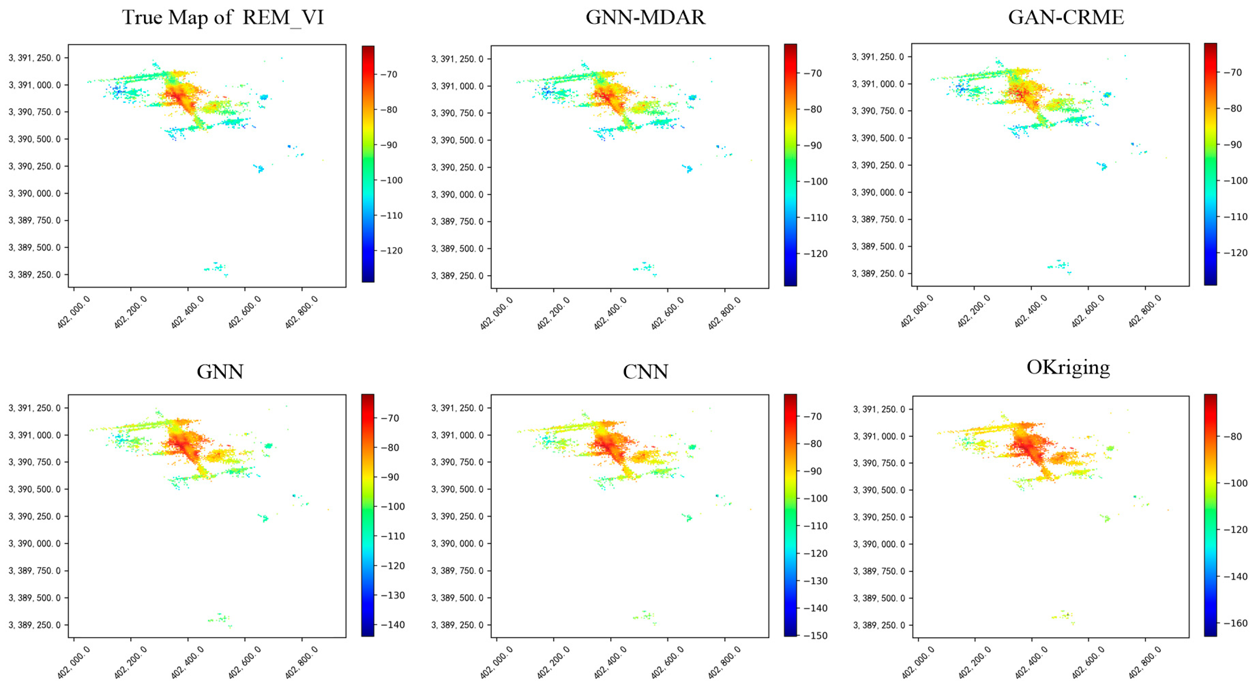
5.2.3. Discussion on the Performance of Four Prediction Models
6. Conclusions and Future Works
Author Contributions
Funding
Data Availability Statement
Acknowledgments
Conflicts of Interest
References
- Miranda, R.F.; Barriquello, C.H.; Reguera, V.A.; Denardin, G.W.; Thomas, D.H.; Loose, F.; Amara, L.S. A Review of Cognitive Hybrid Radio Frequency/Visible Light Communication Systems for Wireless Sensor Networks. Sensors 2023, 23, 7815. [Google Scholar] [CrossRef]
- Beibei, W.; Liu, K.J.R. Advances in cognitive radio networks: A survey. IEEE J. Sel. Top. Signal Process. 2011, 5, 5–23. [Google Scholar] [CrossRef]
- Üreten, S.; Yongaçoğlu, A.; Petriu, E. A comparison of interference cartography generation techniques in cognitive radio networks. In Proceedings of the 2012 IEEE International Conference on Communications (ICC), Ottawa, ON, Canada, 10–15 June 2012; pp. 1879–1883. [Google Scholar]
- Romero, D.; Kim, S.-J. Radio Map Estimation: A data-driven approach to spectrum cartography. IEEE Signal Process. Mag. 2022, 39, 53–72. [Google Scholar] [CrossRef]
- Boccolini, G.; Hernandez-Penaloza, G.; Beferull-Lozano, B. Wireless sensor network for Spectrum Cartography based on Kriging interpolation. In Proceedings of the 2012 IEEE 23rd International Symposium on Personal, Indoor and Mobile Radio Communications—(PIMRC), Sydney, NSW, Australia, 9–12 September 2012; pp. 1565–1570. [Google Scholar]
- Hamid, M.; Beferull-Lozano, B. Non-parametric spectrum cartography using adaptive radial basis functions. In Proceedings of the 2017 IEEE International Conference on Acoustics, Speech and Signal Processing (ICASSP), New Orleans, LA, USA, 5–9 March 2017; pp. 3599–3603. [Google Scholar]
- Dall’Anese, E.; Bazerque, J.A.; Giannakis, G.B. Group sparse Lasso for cognitive network sensing robust to model uncertainties and outliers. Phys. Commun. 2012, 5, 161–172. [Google Scholar] [CrossRef]
- Ding, G.; Wang, J.; Wu, Q.; Yao, Y.-D.; Song, F.; Tsiftsis, T.A. Cellular-Base-Station-Assisted Device-to-Device Communications in TV White Space. IEEE J. Sel. Areas Commun. 2016, 34, 107–121. [Google Scholar] [CrossRef]
- Tang, M.; Ding, G.; Wu, Q.; Xue, Z.; Tsiftsis, T.A. A Joint Tensor Completion and Prediction Scheme for Multi-Dimensional Spectrum Map Construction. IEEE Access 2016, 4, 8044–8052. [Google Scholar] [CrossRef]
- Zhang, G.; Fu, X.; Wang, J.; Hong, M. Coupled Block-term Tensor Decomposition Based Blind Spectrum Cartography. In Proceedings of the 2019 53rd Asilomar Conference on Signals, Systems, and Computers, Pacific Grove, CA, USA, 3–6 November 2019. [Google Scholar]
- Shrestha, S.; Fu, X.; Hong, M. Deep Spectrum Cartography: Completing Radio Map Tensors Using Learned Neural Models. IEEE Trans. Signal Process. 2022, 70, 1170–1184. [Google Scholar] [CrossRef]
- Han, X.; Xue, L.; Shao, F.; Xu, Y. A Power Spectrum Maps Estimation Algorithm Based on Generative Adversarial Networks for Underlay Cognitive Radio Networks. Sensors 2020, 20, 311. [Google Scholar] [CrossRef]
- Zhang, Z.; Zhu, G.; Chen, J.; Cui, S. Fast and Accurate Cooperative Radio Map Estimation Enabled by GAN. arXiv 2024, arXiv:2402.02729. [Google Scholar]
- Levie, R.; Yapar, Ç.; Kutyniok, G.; Caire, G. RadioUNet: Fast Radio Map Estimation with Convolutional Neural Networks. IEEE Trans. Wirel. Commun. 2021, 20, 4001–4015. [Google Scholar] [CrossRef]
- Teganya, Y.; Romero, D. Deep Completion Autoencoders for Radio Map Estimation. IEEE Trans. Wirel. Commun. 2022, 21, 1710–1724. [Google Scholar] [CrossRef]
- Shen, Y.; Zhang, J.; Song, S.H.; Letaief, K.B. Graph Neural Networks for Wireless Communications: From Theory to Practice. IEEE Trans. Wirel. Commun. 2023, 22, 3554–3569. [Google Scholar] [CrossRef]
- Lee, M.; Yu, G.; Dai, H.; Li, G.Y. Graph Neural Networks Meet Wireless Communications: Motivation, Applications, and Future Directions. IEEE Wirel. Commun. 2022, 29, 12–19. [Google Scholar] [CrossRef]
- Eisen, M.; Ribeiro, A. Large Scale Wireless Power Allocation with Graph Neural Networks. In Proceedings of the 2019 IEEE 20th International Workshop on Signal Processing Advances in Wireless Communications (SPAWC), Cannes, France, 2–5 July 2019; pp. 1–5. [Google Scholar]
- Naderializadeh, N.; Eisen, M.; Ribeiro, A. Wireless power control via counterfactual optimization of graph neural networks. In Proceedings of the IEEE 21st International Workshop on Signal Processing Advances in WirelessCommunications (SPAWC), Atlanta, GA, USA, 26–29 May 2020; pp. 1–5. [Google Scholar]
- Zhao, S.; Jiang, X.; Jacobson, G.; Jana, R. Cellular network traffic prediction incorporating handover: A graph convolutional approach. In Proceedings of the 17th Annual IEEE International Conference on Sensing, Communication, and Networking (SECON), Como, Italy, 22–25 June 2020; pp. 1–9. [Google Scholar]
- Chen, G.; Liu, Y.; Zhang, T.; Zhang, J.; Guo, X.; Yang, J. A Graph Neural Network Based Radio Map Construction Method for Urban Environment. IEEE Commun. Lett. 2023, 27, 1327–1331. [Google Scholar] [CrossRef]
- Bufort, A.Y.; Lebocq, L.; Cathabard, S. Data-Driven Radio Propagation Modeling using Graph Neural Networks. TechRxiv 2023. [Google Scholar] [CrossRef]
- Saenko, K.; Kulis, B.; Fritz, M.; Darrell, T. Adapting Visual Category Models to New Domains. In European Conference on Computer Vision; Springer: Berlin/Heidelberg, Germany, 2010; Volume 6314, pp. 213–226. [Google Scholar]
- Jiang, J.; Ji, Y.; Wang, X.; Liu, Y.; Wang, J.; Long, M. Regressive Domain Adaptation for Unsupervised Keypoint Detection. In Proceedings of the 2021 IEEE/CVF Conference on Computer Vision and Pattern Recognition (CVPR), Nashville, TN, USA, 19–25 June 2021; pp. 6776–6785. [Google Scholar]
- Hoffman, M.; Blei, D.M.; Wang, C.; Paisley, J. Stochastic Variational Inference. Comput. Sci. 2012, 14, 1303–1347. [Google Scholar]
- Goodfellow, I.; Pouget-Abadie, J.; Mirza, M.; Xu, B.; Warde-Farley, D.; Ozair, S.; Courville, A.; Bengio, Y. Generative Adversarial Nets. In Proceedings of the 27th International Conference on Neural Information Processing Systems, Montreal, QC, Canada, 8–13 December 2014; Volume 2, pp. 2672–2680. [Google Scholar]
- Qu, H.; Xu, L.; Cai, Y.; Foo, L.G.; Liu, J. Heatmap Distribution Matching for Human Pose Estimation. arXiv 2022, arXiv:2210.00740. [Google Scholar]
- Zhang, C.; Cai, Y.; Lin, G.; Shen, C. DeepEMD: Few-Shot Image Classification With Differentiable Earth Mover’s Distance and Structured Classifiers. In Proceedings of the 2020 IEEE/CVF Conference on Computer Vision and Pattern Recognition (CVPR), Seattle, WA, USA, 13–19 June 2020; pp. 12200–12210. [Google Scholar]
- Peng, H.; Sun, M.; Li, P. Optimal Transport for Long-Tailed Recognition with Learnable Cost Matrix. In Proceedings of the International Conference on Learning Representations, Virtual, 25–29 April 2022. [Google Scholar]
- Schulter, S.; Vernaza, P.; Choi, W.; Chandraker, M. Deep Network Flow for Multi-object Tracking. In Proceedings of the 2017 IEEE Conference on Computer Vision and Pattern Recognition (CVPR), Honolulu, HI, USA, 21–26 July 2017; pp. 2730–2739. [Google Scholar]
- de Mathelin, A.; Richard, G.; Deheeger, F.; Mougeot, M.; Vayatis, N. Adversarial Weighting for Domain Adaptation in Regression. In Proceedings of the 2021 IEEE 33rd International Conference on Tools with Artificial Intelligence (ICTAI), Washington, DC, USA, 1–3 November 2021; pp. 49–56. [Google Scholar]
- Chen, X.; Wang, S.; Wang, J.; Long, M. Representation Subspace Distance for Domain Adaptation Regression. In Proceedings of the 38th International Conference on Machine Learning, PMLR, Virtual, 18–24 July 2021; Volume 139, pp. 1749–1759. [Google Scholar]
- Kutbi, M.; Peng, K.-C.; Wu, Z. Zero-Shot Deep Domain Adaptation with Common Representation Learning. IEEE Trans. Pattern Anal. Mach. Intell. 2022, 44, 3909–3924. [Google Scholar] [CrossRef] [PubMed]
- Wang, B.; Mendez, J.A.; Cai, M.B.; Eaton, E. Transfer learning via minimizing the performance gap between domains. In Proceedings of the 33rd International Conference on Neural Information Processing Systems, Vancouver, BC, Canada, 8–14 December 2019; pp. 10645–10655. [Google Scholar]
- Singh, A.; Chakraborty, S. Deep Domain Adaptation for Regression. In Development and Analysis of Deep Learning Architectures; Pedrycz, W., Chen, S.-M., Eds.; Springer International Publishing: Cham, Switzerland, 2020; pp. 91–115. [Google Scholar]
- NT, H.; Maehara, T.; Murata, T. Revisiting Graph Neural Networks: Graph Filtering Perspective. In Proceedings of the 2020 25th International Conference on Pattern Recognition (ICPR), Milan, Italy, 10–15 January 2021; pp. 8376–8383. [Google Scholar]
- Zhou, Z.; Meng, L.; Tang, C.; Zhao, Y.; Chen, W. Visual Abstraction of Large Scale Geospatial Origin-Destination Movement Data. IEEE Trans. Vis. Comput. Graph. 2019, 25, 43–53. [Google Scholar] [CrossRef] [PubMed]
- Wen, X.; Fang, S.; Xu, Z.; Liu, H. Joint Multidimensional Pattern for Spectrum Prediction Using GNN. Sensors 2023, 23, 8883. [Google Scholar] [CrossRef] [PubMed]
- Chen, D.; Zhu, H.; Yang, S.; Dai, Y. Unsupervised multi-source domain adaptation with graph convolution network and multi-alignment in mixed latent space. Signal Image Video Process. 2023, 17, 855–863. [Google Scholar] [CrossRef]
- Sun, Q.; Li, J.; Peng, H.; Wu, J.; Fu, X.; Ji, C.; Yu, P.S. Graph Structure Learning with Variational Information Bottleneck. arXiv 2021, arXiv:2112.08903. [Google Scholar] [CrossRef]
- Cover, T.M.; Thomas, J.A. Elements of Information Theory, 1st ed.; Tsinghua University Press: Beijing, China, 2006. [Google Scholar]
- Yoo, J.; Jeon, H.; Jung, J.; Kang, U. Accurate Node Feature Estimation with Structured Variational Graph Autoencoder. In Proceedings of the 28th ACM SIGKDD Conference on Knowledge Discovery and Data Mining, Washington, DC, USA, 14–18 August 2022. [Google Scholar]
- Du, Y.; Wang, J.; Feng, W.; Pan, S.; Qin, T.; Xu, R.; Wang, C. AdaRNN: Adaptive Learning and Forecasting of Time Series. In Proceedings of the 30th ACM International Conference on Information and Knowledge Management, New York, NY, USA, 1–5 November 2021; pp. 402–411. [Google Scholar]
- Gretton, A.; Sriperumbudur, B.; Sejdinovic, D.; Strathmann, H.; Kenji, F. Optimal kernel choice for large-scale two-sample tests. In Proceedings of the Advances in Neural Information Processing Systems 25 (NIPS 2012), Lake Tahoe, NV, USA, 3–6 December 2012; pp. 1205–1213. [Google Scholar]
- Ganin, Y.; Ustinova, E.; Ajakan, H.; Germain, P.; Larochelle, H.; Laviolette, F.; Marchand, M.; Lempitsky, V. Domain-Adversarial Training of Neural Networks. In Domain Adaptation in Computer Vision Applications; Csurka, G., Ed.; Springer International Publishing: Cham, Switzerland, 2017; pp. 189–209. [Google Scholar]
- Hashimoto, R.; Suto, K. SICNN: Spatial Interpolation with Convolutional Neural Networks for Radio Environment Mapping. In Proceedings of the 2020 International Conference on Artificial Intelligence in Information and Communication (ICAIIC), Fukuoka, Japan, 19–21 February 2020; pp. 167–170. [Google Scholar]


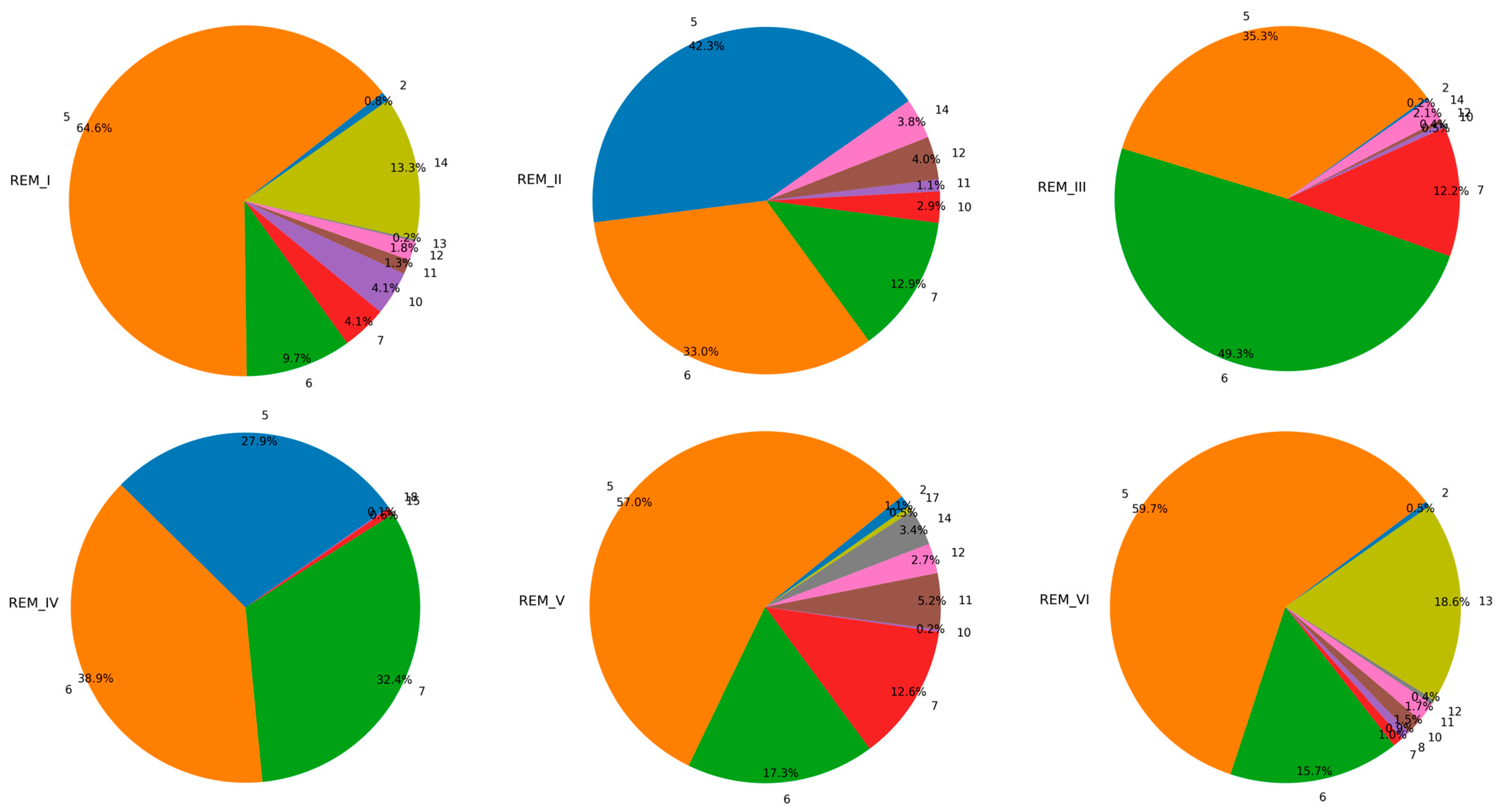
| Index | Type of Clutter | Index | Type of Clutter |
|---|---|---|---|
| 1 | Oceans and Coastlines | 11 | High-rise Urban Buildings (40 m–60 m) |
| 2 | Lakes and Rivers | 12 | Middle and High-rise Buildings in Urban Areas (20 m–40 m) |
| 3 | Wetlands and Marshes | 13 | High-density Building Complex (<20 m) in Urban Areas |
| 4 | Suburban Open Areas | 14 | Multi-story Buildings (<20 m) in Urban Areas |
| 5 | Urban Open Areas | 15 | Low-density Industrial Building Areas |
| 6 | Roadside Open Areas | 16 | High-density Industrial Building Areas |
| 7 | Grasslands or Pastures | 17 | Suburbs |
| 8 | Shrub Vegetation | 18 | Developed Suburban Areas |
| 9 | Forest Vegetation | 19 | Rural Areas |
| 10 | Supertall Urban Buildings (>60 m) | 20 | CBD Commercial Zone |
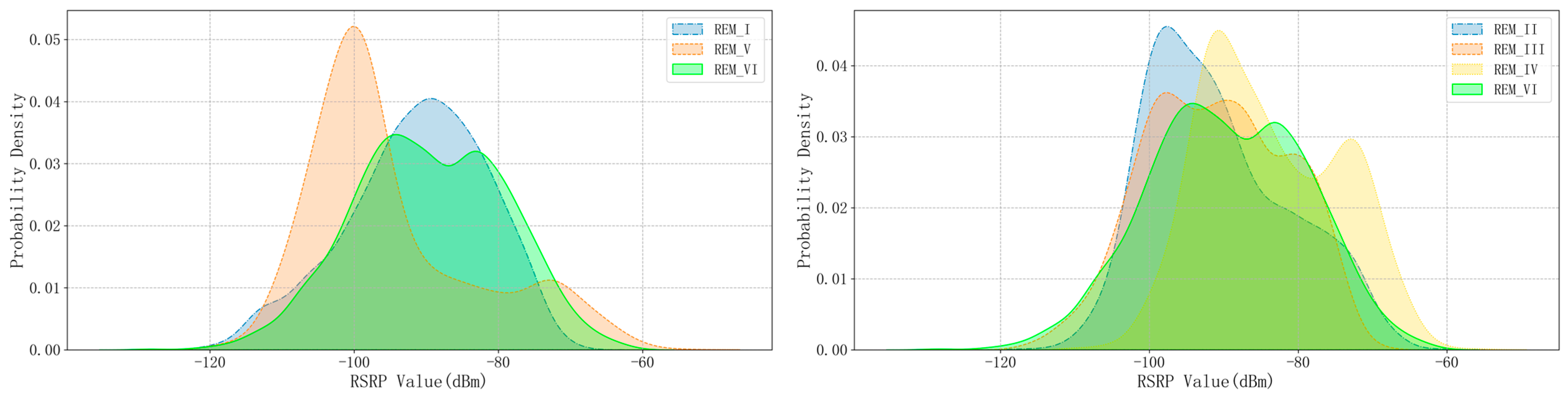
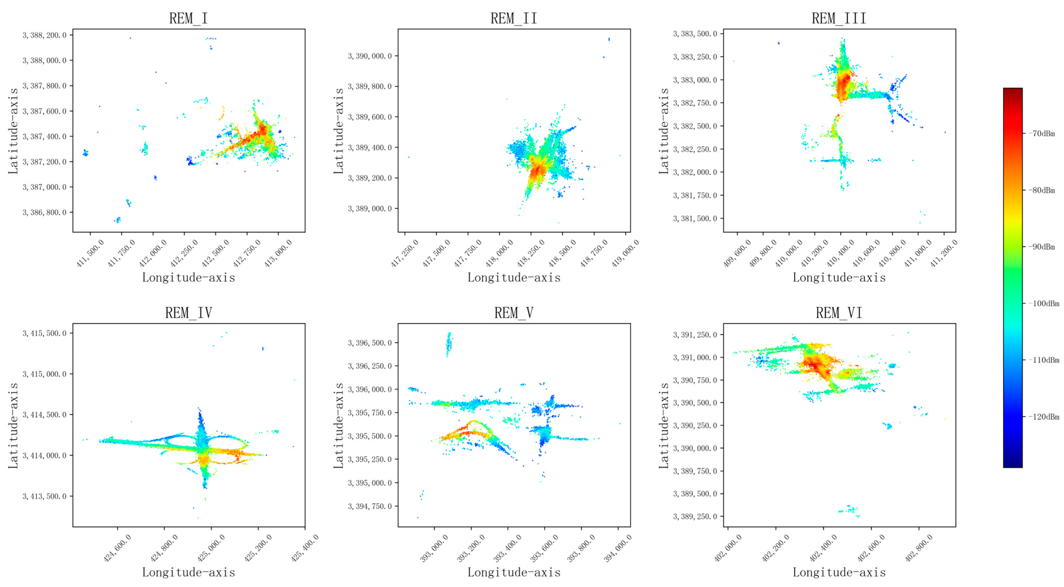
| REM ID | Number of Grids | RSRP Statistical Distribution | |
|---|---|---|---|
| Mean Value | Variance | ||
| I | 2483 | −91.21 dBm | 93.74 dBm |
| II | 3327 | −90.75 dBm | 90.74 dBm |
| III | 3837 | −90.97 dBm | 88.89 dBm |
| IV | 3612 | −88.88 dBm | 86.08 dBm |
| V | 2312 | −94.72 dBm | 143.45 dBm |
| VI | 2053 | −89.53 dBm | 109.78 dBm |
| Methods | Datasets | MAE | RMSE | MAPE(%) |
|---|---|---|---|---|
| Kriging | REM_VI | 24.45 | 30.11 | 21.15 |
| CNN | REM_V, REM_VI | 16.63 | 19.02 | 14.12 |
| GNN | REM_V, REM_VI | 15.26 | 18.71 | 13.83 |
| REM_I, REM_V, REM_VI | 15.05 | 17.93 | 13.08 | |
| GAN-CRME | REM_I, REM_V, REM_VI | 11.45 | 16.03 | 14.16 |
| REM_II, REM_III, REM_IV, REM_VI | 8.71 | 12.53 | 10.24 | |
| GNN-MDAR | REM_I, REM_V→REM_VI | 10.31 | 13.57 | 8.42 |
| REM_II, REM_III, REM_IV→REM_VI | 7.28 | 8.49 | 6.07 |
Disclaimer/Publisher’s Note: The statements, opinions and data contained in all publications are solely those of the individual author(s) and contributor(s) and not of MDPI and/or the editor(s). MDPI and/or the editor(s) disclaim responsibility for any injury to people or property resulting from any ideas, methods, instructions or products referred to in the content. |
© 2024 by the authors. Licensee MDPI, Basel, Switzerland. This article is an open access article distributed under the terms and conditions of the Creative Commons Attribution (CC BY) license (https://creativecommons.org/licenses/by/4.0/).
Share and Cite
Wen, X.; Fang, S.; Fan, Y. Reconstruction of Radio Environment Map Based on Multi-Source Domain Adaptive of Graph Neural Network for Regression. Sensors 2024, 24, 2523. https://doi.org/10.3390/s24082523
Wen X, Fang S, Fan Y. Reconstruction of Radio Environment Map Based on Multi-Source Domain Adaptive of Graph Neural Network for Regression. Sensors. 2024; 24(8):2523. https://doi.org/10.3390/s24082523
Chicago/Turabian StyleWen, Xiaomin, Shengliang Fang, and Youchen Fan. 2024. "Reconstruction of Radio Environment Map Based on Multi-Source Domain Adaptive of Graph Neural Network for Regression" Sensors 24, no. 8: 2523. https://doi.org/10.3390/s24082523
APA StyleWen, X., Fang, S., & Fan, Y. (2024). Reconstruction of Radio Environment Map Based on Multi-Source Domain Adaptive of Graph Neural Network for Regression. Sensors, 24(8), 2523. https://doi.org/10.3390/s24082523