1. Introduction
In 5G and beyond, massive businesses with strict reliability requirements surge, which expects extensive bandwidth provisioning. This will lead to more severe spectrum shortages. Visible light communication (VLC) is a potential paradigm to ease the dilemma of radio frequency (RF) resources in the next-generation communication systems [
1,
2]. Benefiting from the characteristics of light, VLC can provide high transmission rates, ultra-wide frequency bands, high-energy efficiency, low cost, and indoor full coverage. It can be deployed as indoor high-speed data links for personal area networks and RFs in non-friendly environments. In critical scenarios, such as remote control in medical operating rooms and factory automation under strong magnetic interference, VLC is expected to embrace massive services with traffic possessing strong randomness, heterogeneity, and burstiness [
3]. The data require the reliability of latency within the millisecond level to reach 99.99–99.999% [
4,
5]. For traffic featuring complex characteristics transmitted on visible light channels, we should explore an effective and precise evaluation method of reliability with regard to latency, which can reveal the influence of entanglement between visible light data traffic and visible light transmission schemes. Meanwhile, an efficient routing strategy needs to be explored for the VLC network.
In the VLC wireless network, the light-emitting diode (LED) access point (AP) carries packet flows from different services, which possess heterogeneous characteristics [
6,
7]. The convergence of heterogeneous visible light data flows intensifies the uncertainty of the aggregate traffic. In [
8], the aggregate traffic was composed of multiple 2-state Markov-modulated Bernoulli processes (MMBP-2) and was tackled as one MMBP-2 by the Kronecker product operation. The proposed method is not of universal applicability and is unable to provide a theoretical result of the latency-bounded reliability. The stochastic network calculus (SNC) theory, effective bandwidth (EB), and effective capacity (EC) theories provide classical analysis methods of latency-bounded reliability. The union-bound inequality, as the key enabler in SNC, only supports capturing a loose upper bound of unreliability [
9]. In the EB/EC framework, the stochastic traffic is tackled as a constant flow [
10,
11], which always triggers rougher theoretical results of latency performance, especially for bursty traffic.
Martingale, a random process throughout modern probability theory, has demonstrated great superiority in the precise analysis of the statistical reliability regarding latency. The theoretical upper bounds of unreliability derived in [
9,
12] are more precise than the existing conclusions. This martingale-based analysis framework is a milestone. In [
13,
14], the latency-bounded unreliability of the Markov-modulated on–off (MMOO) arrival process was analyzed in the ALOHA access scheme. Based on the results, the bandwidth resources were allocated reasonably. More importantly, martingales have been explored to support the evaluation of the end-to-end reliability of latency. In [
15], a precise analysis framework of the end-to-end latency-bounded unreliability was introduced, where a multi-hop routing path was considered and the traffic was modeled as a Markov-modulated process. Then, the proposed method was extended in the 6G network scenarios [
16]. For the system adopting the THz wireless access scheme, the end-to-end latency performance was analyzed for the traffic generated from virtual reality. In [
17], we constructed an analysis framework of latency performance for the aggregate traffic, which was constituted by the heterogeneous Markov-modulated flows. The martingale of the queuing length was defined, and the latency-bounded unreliability was derived.
These remarkable conclusions have inspired our work on the statistical latency QoS analysis based on martingale theory. The framework in [
17] is theoretical without specific application scenarios. In this paper, the latency analysis in the VLC network is focused on. The differences with [
17] can be summarized as follows. (1) The cross-layer service process is modeled, which is the improvement of the proposed method in [
17]. Specifically, in the physical layer, the Lambertian sources are considered and the channel gain is depicted. The Shannon Theorem is leveraged to model the achievable transmission rates, which achieves the mapping between the physical layer and the data link layer. We focus on the characteristic that the VLC links are easy to block. Blocking the line of sight (LoS) between the VLC AP and the targeted terminal at each time slot is considered a random variable, which triggers the stochastic features of the service process and further impacts the latency of the aggregate traffic. (2) Meanwhile, the martingale process related to latency is a proposed novelty, which is another way to analyze latency different from [
17]. It introduces the statistical characteristics of the service scheme and data traffic into martingale parameters, which reveals the influence of random blocks of the VLC link and the burstiness of aggregate traffic on the latency. (3) The stopping time event about latency is defined, which is the time point when the system latency exceeds the threshold. Applying the stopping time theory to the latency-related martingale, the upper bound of the unreliability with regard to latency is captured. (4) More importantly, the end-to-end reliability provisioning is investigated in this paper, not just the air interface latency analysis.
Further, for the aggregate traffic forwarded by the VLC AP, an efficient routing algorithm is proposed based on the back-pressure theory in the core network. Some studies have investigated the utilization of back-pressure theory to improve network performance, specifically within the Transmission Control Protocol domain [
18]. Additionally, alternative research has concentrated on employing back-pressure algorithms to facilitate relay selection in wireless sensor networks and wireless multi-hop networks [
19]. Although the source node (LED access point) can adopt the classic back-pressure algorithm to promote the network capacity, the classic algorithm results in significant packet delays and poor node energy. Therefore, combining the latency performance analysis, we design a new link weight calculation method to make routing and scheduling decisions, which considers the data packet’s recent node record, the neighbor node’s remaining energy status, and the queue latency. Meanwhile, we note that no prior research has explored the integration of back-pressure theory in visible light network systems.
To summarize, in this paper, considering the VLC APs serve the aggregate traffic with burstiness, a precise analysis framework of the latency-bounded reliability is proposed. In the core network, an efficient routing algorithm is introduced for the complex aggregate traffic. The contributions can be concluded as follows.
The service process of the VLC network and the aggregate arrival process are modeled in the martingale domain. For the VLC link with a random block, the i.i.d. service process provided by the LED AP is considered. Through mapping the statistical features of random block behavior in the martingale parameters, the martingale of the service is constructed. Leveraging the relation between the spectral radius and the eigenvector in Markov chains, martingales of Markov-modulated arrival processes are defined.
We propose a martingale process related to latency, which models the impact of entanglement between complex arrivals and random service on the latency. A stopping time point at which the latency violates the threshold is considered. Based on the stopping time theory, the complementary cumulative distribution function of latency is obtained for the VLC network. We evaluate the latency in terms of burstiness, which is measured by the squared coefficient of variation.
When the LED AP node data reach the core network, a dynamic back-pressure algorithm based on energy and latency from aggregate traffic is proposed, which designs a new link weight calculation method to make routing and scheduling decisions. The modified back-pressure algorithm trades off three factors, including the data packet’s recent node record, the neighbor node’s remaining energy status, and the queue latency, to boost the network performance and data transmission quality. Meanwhile, our scheme is the first research to apply back-pressure theory in the visible light network.
2. The Network Model and the Queuing System
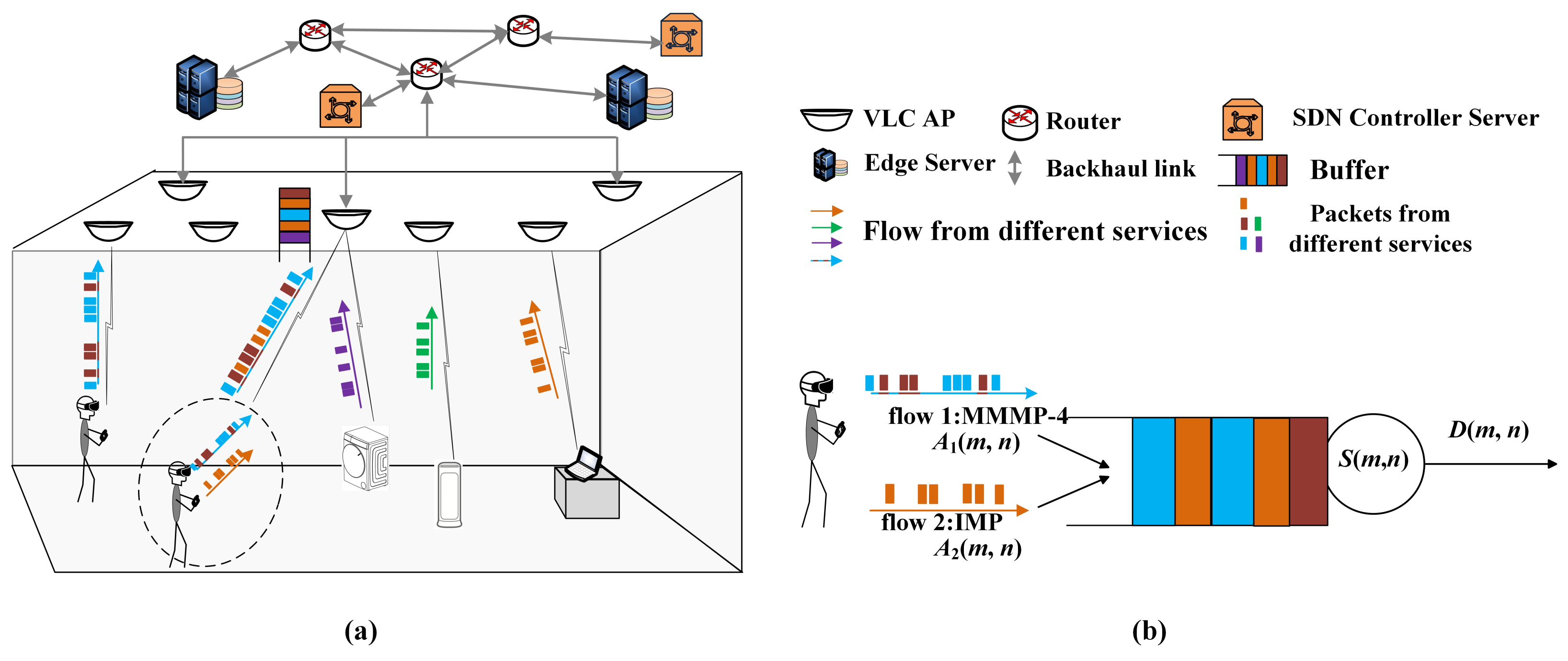
We consider a multi-service uplink communication scenario, as shown in
Figure 1. The data flow from different services (business) is statistically heterogeneous. That is, diverse models are adopted to describe the randomness of flows. The data packets belonging to different flows could access the same VLC AP, where these flows compose the aggregate traffic. The targeted AP supplies the transmission rates for the aggregate traffic according to a specific scheme. Because of the randomness of the VLC channel and the block, the transmission process provided for the aggregate traffic is stochastic. Thus, the backlog and latency are triggered in the buffer of the targeted VLC AP.
- A.
The queuing system of aggregate traffic
In the VLC access network, the target terminal is associated with the nearest VLC AP. This terminal carries two services where the generated packet flows are heterogeneous. Thus, the aggregate traffic is transmitted from this terminal, as shown in
Figure 1a. We consider the block of LoS between the VLC AP, and this terminal obeys a Bernoulli distribution of parameter
. Then, the channel gain can be modeled as
where
b is the Lambertian index, and
.
is the half-intensity radiation angle.
is the area of reviewer photodetector (PD).
d is the distance between the AP and the terminal.
is the gain of the optical filter.
and
are the angle of incidence and irradiance between VLC AP and the terminal, respectively.
is the optical concentrator gain, which is a function of
where
r is the refractive index, and
is the semi-angle of the field of view (FoV) of the PD.
Based on the Shannon theorem, the achievable transmission rate between AP and the terminal, which is defined as
, can be given as
where
is the system bandwidth, and
is the transmission power.
is the noise power.
The access process of the packets from aggregate traffic can be modeled as a queuing system, as is presented in
Figure 1b. These two flows constituting the aggregate traffic are independent and described as the four-state Markov-modulated multinomial process (MMMP-4) and the interrupted multimomial process (IMP), respectively, which are introduced in part B in detail. These are the arrival processes of the queuing system. The access process is modeled as the service process provided by the AP. Because latency is often described in units of packets, the arrival process and the service process are modeled from the perspective of packets/slots. Without loss of generality, the length of packets is assumed to be fixed. The flows from different services have the same priority. Thus, the first-in-first-out (FIFO) scheduling scheme is adopted in the buffer.
In
Figure 1b,
is the accumulated arrival processes in
of flow
i.
can be written as
, where
is the number of arrival packets of flow
i at time slot
k. The arrival process
is modeled as an MMMP-4, and
is modeled as an IMP, which are bursty and heterogeneous. Let
denote the aggregate accumulated arrival process from slot
m to slot
n. Similarly, the accumulated service process
provided by the VLC AP is also a bivariate process,
, where
is the service process.
is the number of the served packets at slot
n. In this paper,
is a random variable following a Bernoulli distribution with successful probability
p and service rate
C.
can be given by
where
.
T s/slot is the duration of a slot and
L bits/packet is the length of a packet. To simplify the subsequent analysis,
C is assumed as a constant.
Based on SNC, the departure process
can be defined by
and
using (min, +) convolution. The backlog process
in the buffer is defined as
and the latency
at slot
n is
- B.
The heterogeneous arrival models
The MMMP-4 is proposed to describe the interweaving arrival characteristics of packet flows from different services in a terminal. A 2D Markov chain is considered, which is denoted as
.
represents the service that generates the packets.
models whether there are packets generated at time slot
n.
means that no packet is arriving, while
means that packets are generated. Corresponding to
and
, packet arrival probabilities at each slot are
and
, respectively. If service
generates packets at slot
n, the number of packets is
, and in the other case, it is
. Thus, the state space of the MMMP-4 model is
. The state transition probabilities between two services,
and
, are
and
, respectively. Based on [
17], the state transition matrix of the 2D Markov chain is defined as
.
The IMP model is proposed to embody the bursty and sporadic arrival characteristics of the small data service. It is also a 2D Markov chain, which is denoted as
.
.
represents the service that generates the packets. In state
, there are no packets generated.
describes whether there are packets at slot
n.
represents that no packet arrives in state
, and
represents that
packets arrive in state
. It is worth noting that
means that no packets arrive in idle state
with probability one. The state space of the IMP model is
. The state transition probabilities between
and
are
and
, respectively. In
, the packet generation process is stochastic and follows a multinomial distribution with the arrival probability
and the number of arrival packets
. The state transition matrix of the IMP is
. The MMMP-4 model and IMP model are shown in [
17].
3. Martingale-Based Latency-Bounded Reliability Analysis
The arrival and service processes are described by martingales in this part. The upper bound of the latency-bounded unreliability is analyzed based on the stopping theory.
- A.
Martingale constructions of arrival and service processes
Firstly, we introduce the definition of martingales.
Definition 1 (martingales)
. Let be a probability space and be a filtration, i.e., a non-decreasing sequence of σ-fields of , . A random sequence is adapted to . That is, is measurable with respect to . If
- (1)
- (2)
,
holds, then is a martingale sequence.
Further, if , then is a supermartingale.
As a powerful mathematical method, martingales can provide us with a framework to depict heterogeneous arrivals with burstiness. Martingale processes are inclusive, which shows that other random processes are transformed as martingale processes by martingale construction. Meanwhile, martingale can provide a modularized description method for arrival and service processes, which contributes to the model, analyzes the features of the backlog process (the difference between two random processes), and further enables the analysis of latency for aggregate traffic. It is noted that the inequality formulary of martingales supports the upper bound analysis of unreliability with regard to latency naturally. We construct the martingale processes of arrival and service, respectively, as follows.
Definition 2 (Martingale of arrival)
. Consider a Markov process , which is -measurable. The state space is . The state transition matrix is . . The arrival process is Markov modulated, i.e., and . Define a -transform for as . . The spectral radius of is , and the corresponding eigenvector is . The random processis constructed as a martingale relative to . Then, is admitted as a martingale of arrival . The function is We use the definition of martingales to prove Definition 2.
Proof. It is obvious that
and
. Thus,
holds. We can write that
(a) is from the basic operation of conditional expectation and the definition of
.
is the
ith element of vector
. Then, (b) holds due to the relation between the eigenvector and eigenvalue, i.e.,
, and the definition of
. □
For the MMMP-4 and IMP models, the martingale parameters are
,
, and
,
respectively, which are related to
and
. The corresponding specific formulas can refer to [
17].
Similar to the martingale of arrival, the martingale of the i.i.d. service process is constructed as described in Definition 3.
Definition 3 (Martingale of service)
. The service process is , which is -measurable. The moment generating function is . The accumulated service process of is . Then, the random processis constructed as a martingale relative to . is admitted as a martingale of service . The function is Proof. According to
, we can get
. Meanwhile,
(a) is because of the i.i.d. property. To support formula (b),
is set as a constant. The proof is completed based on
. □
Based on the characteristics of martingale processes, the backlog process can be modeled in the martingale domain, which facilitates the analysis of the latency performance.
Definition 4 (Martingale of backlog)
. The martingales of arrival and service are defined as Definition 2 and 3. Define the product of (7) and (10) as the martingale of backlog by the restriction of ,where . - B.
The latency-bounded unreliability
Theorem 1. Consider a link for the aggregate traffic. The service process is modeled as . The aggregate traffic is . The martingale of arrival is defined by Definition 2, and the martingale of service is in Definition 3. Then, the latency-bounded unreliability of the link holds for ,where . k is the latency threshold. The proof of Theorem 1 is based on the stopping time theory of martingale, as shown in Theorem 2 of [
17].
Proof. Define a stopping time
T for the martingale of backlog
, which is the first time that the backlog exceeds threshold
, i.e.,
. Let
. For
, Theorem 2 is used. The probability of system backlog exceeding threshold
can be obtained
The detailed derivation process can refer to [
17]. Based on the definition of the departure process, the latency-bounded probability,
can be transformed as follows.
According to the time shift feature of martingales, it is obvious that
is also a martingale process.
can be regarded as a martingale related to latency. To complete the latency analysis, the stopping time event about latency is defined as
and can be transformed as
Then, the first time slot that
occurs is the stopping time
.
Combined with the derivation of (
15) and renting the stopping time theory for the martingale process
, we can derive that
When
, we can obtain
. The proof is completed. □
4. Relay Selection for Visible Light Network
We assume that the visible light network is represented by . V is the set of all nodes in the network, and L is the set of all links in the network. The nodes are static and the communication links are bidirectional. The topology changes as nodes die or links fail. All visible light nodes have the same configuration.
We set the network operation by time sharing, i.e., . At each time slot t, the back-pressure algorithm activates a set of interference-free links in the network. When the new data arrive in the network, each node makes routing and transmission scheduling decisions, and the visible light packets are delivered to the appropriate destinations. The back-pressure algorithm divides the visible light packet types according to the difference in the destination. Each packet in the network records information about the source and destination nodes. is denoted as the total number of packet types on node i at time slot t. If , then , indicating that node i is the destination node for the d number packets. Each node maintains up to N (total number of nodes) queues for storing packets arriving at different destination nodes.
is denoted as the set of link scheduling, and denotes the set of all schedulable links under the interference condition. The back-pressure algorithm used in the visible light network is as follows.
STEP-1: Calculating the weights of the links. The link
is any link in the network, the node
n is a neighboring node of the node
m within the network communication range, and
d is the destination node in the network. We calculate the backlog difference of different kinds of packets between node
m and node
n, while the value of the backlog difference must be the positive integer, as follows,
where
denotes the backlog difference of the packet queue of node
d between node
m and node
n at time slot
t.
and
are the queue length values for node
m and node
n, respectively.
We select the maximum value of all the queue backlog differences as the weight of the link, as follows,
where
D is the set of all destination nodes.
is a maximum value in the set of all different kinds of packet queue backlog differences
. At time slot
t, we make
as the optimal packet with
value for link
.
STEP-2: Selecting schedulable links. We set the optimization function as follows,
where
denotes the set of all schedulable links under the interference model.
is the link transmission rate.
is the set of optimal transmission links.
STEP-3: Selecting routing paths. At time slot t, link under the routing and scheduling policy, we transmit the optimal kind of packet from node m to node n.
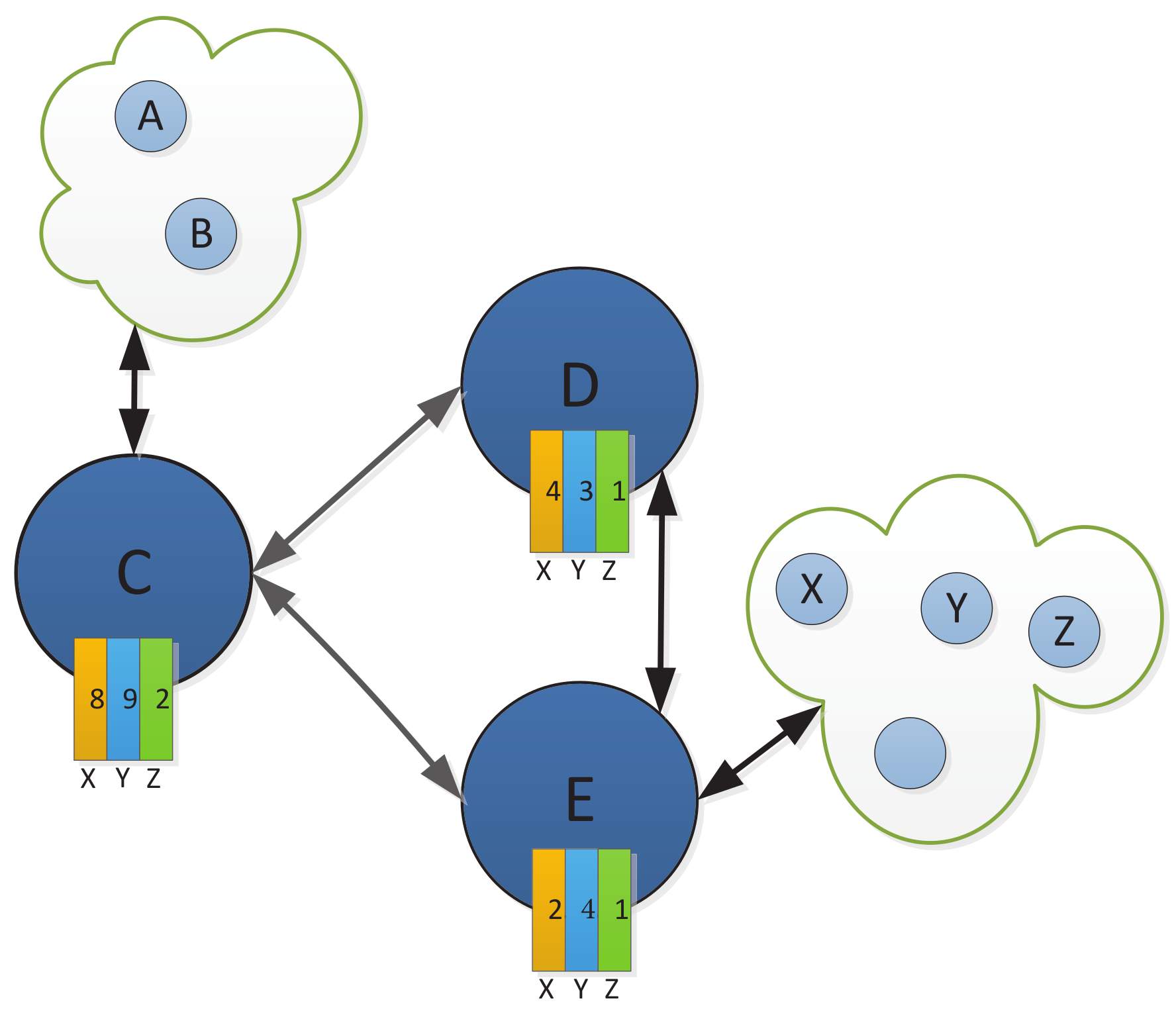
The back-pressure algorithm for the relay selection in the visible light network is shown in Algorithm 1. We illustrate the workflow of the algorithm with a simple example.
Figure 2 shows a visible light communication uploading network. There are three relay nodes
C,
D, and
E, and three different destinations
X,
Y, and
Z. From the figure, we can see the backlog number, i.e., the queue length value, corresponding to each packet type at each node, as shown in
Table 1. We assume that the link
rate is
packets/slot, and the link
rate is
packets/slot. The neighboring node
C at time slot
t are only
D and
E.
| Algorithm 1 The back-pressure algorithm for the relay selection in visible light network |
- Input:
, m, Web G, Node m, Link rate - Output:
Routing strategy - 1:
procedure Original back-pressure ▹Calculate Weight - 2:
for all links do - 3:
for all doPacket type d - 4:
- 5:
end for - 6:
- 7:
- 8:
Packet types with maximum weight - 9:
end for ▹ Link Scheduling - 10:
for all do - 11:
The sum of the products of link weight and rate - 12:
end for - 13:
▹ Data Transferring - 14:
for all do - 15:
transfer packets from m to n - 16:
end for - 17:
end proceduce
|
First, we use Equation (
21) to compute the queue backlog difference for different kinds of packets
X,
Y, and
Z for link
and link
, respectively. The values of queue backlog difference for different kinds of packets are shown in
Table 2.
Then, we calculate the weights of the two links
and
, respectively, by Equation (
22); the results are shown in
Table 3.
Next, we derive the schedulable links. At time slot t, for node C, the link scheduling sets and interfere with each other, they cannot be scheduled simultaneously. The rate of link is packets/slot, the rate of link is packets/slot, and , . We can find that , so we select link . The optimal data packet type is Y and the optimal transmission rate is .
Finally, at time slot t, the routing decision of node C is that packets of type Y will be transmitted to node D at a rate of 4 packets/slot through link for several packets.
5. Simulations and Results Analysis
Firstly, the derived theoretical result is evaluated in part A, and the relay selection algorithm is analyzed in part B.
- A.
The theoretical upper bound of the unreliability of latency
The dynamic change of packets in the queuing system is simulated, where the arrival process models the aggregate traffic. The simulation results of the latency-bounded unreliability are measured by the ratio of the number of slots where the latency exceeds the threshold to the total observation slots.
In
Figure 3, the aggregate arrival process is composed of an MMMP-4 process and an IMP process. The service process is modeled as a geometric distribution. The model parameters are summarized in Nomenclature section. The upper bounds of unreliability regarding latency with different system load
is presented, where
is defined as the ratio of the average arrival rate to the average service rate. According to the system load, the corresponding service rate
C can be determined. The simulation results of unreliability are presented by box plots. It can be shown that the upper bounds of unreliability with regard to latency match the simulated results well with different
. The analysis framework can provide effective results of latency performance for the aggregate traffic with heterogeneity and burstiness. Obviously, the system load plays a significant role in the reliability. In the heavy-load system (
), the latency-bounded reliability is terrible such that it cannot support almost any services with statistical reliability requirement even if the latency threshold is large.
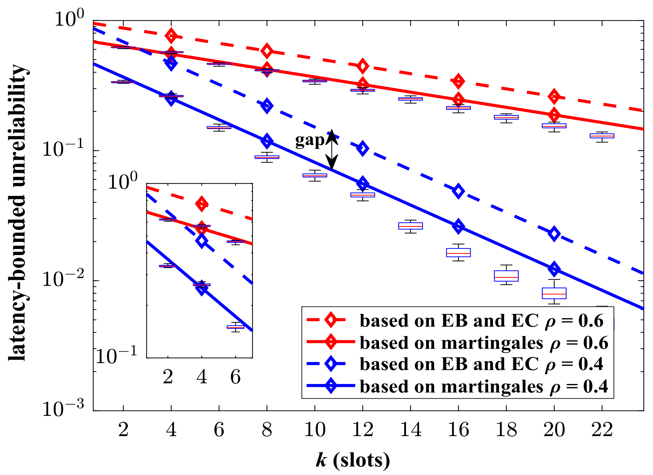
In order to verify the advantages of the proposed analysis framework, we compare the theoretical results with the state-of-the-art ones based on EB/EC theory in
Figure 4. In this part, the aggregate traffic consists of two identical MMOO processes. The parameters of the MMOO model are listed in Nomenclature section. The result based on the EB/EC theory refer to [
20]. It can be shown that the upper bound of unreliability obtained in this paper is much tighter than the compared one. The martingale-based theoretical results match the simulations well. The gap between the EB/EC-based results and the simulated values is obvious. Our analysis method can provide a more precise analysis for the latency performance of the Markovian aggregate traffic. The EB/EC theory assumes bursty traffic as the constant fluid, which makes it impossible to reflect the influence of complex random characteristics of aggregate traffic on latency performance.
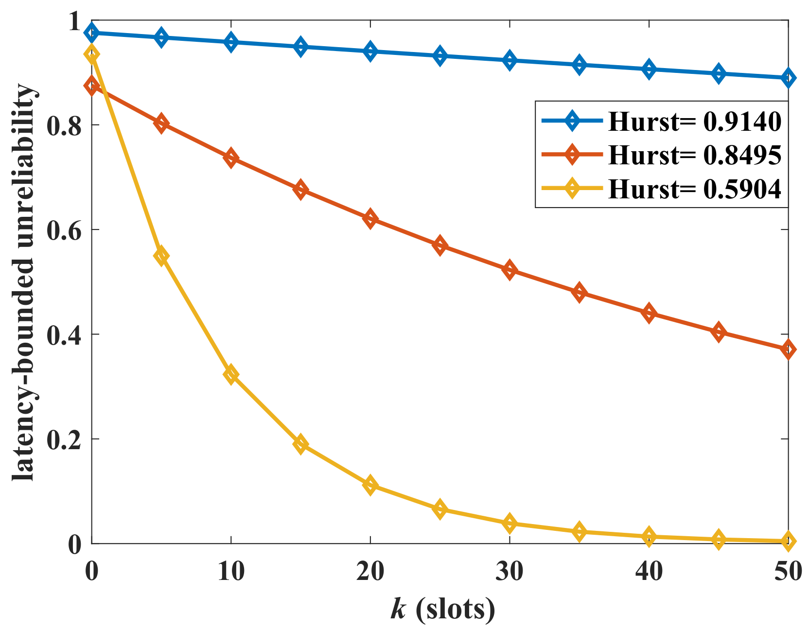
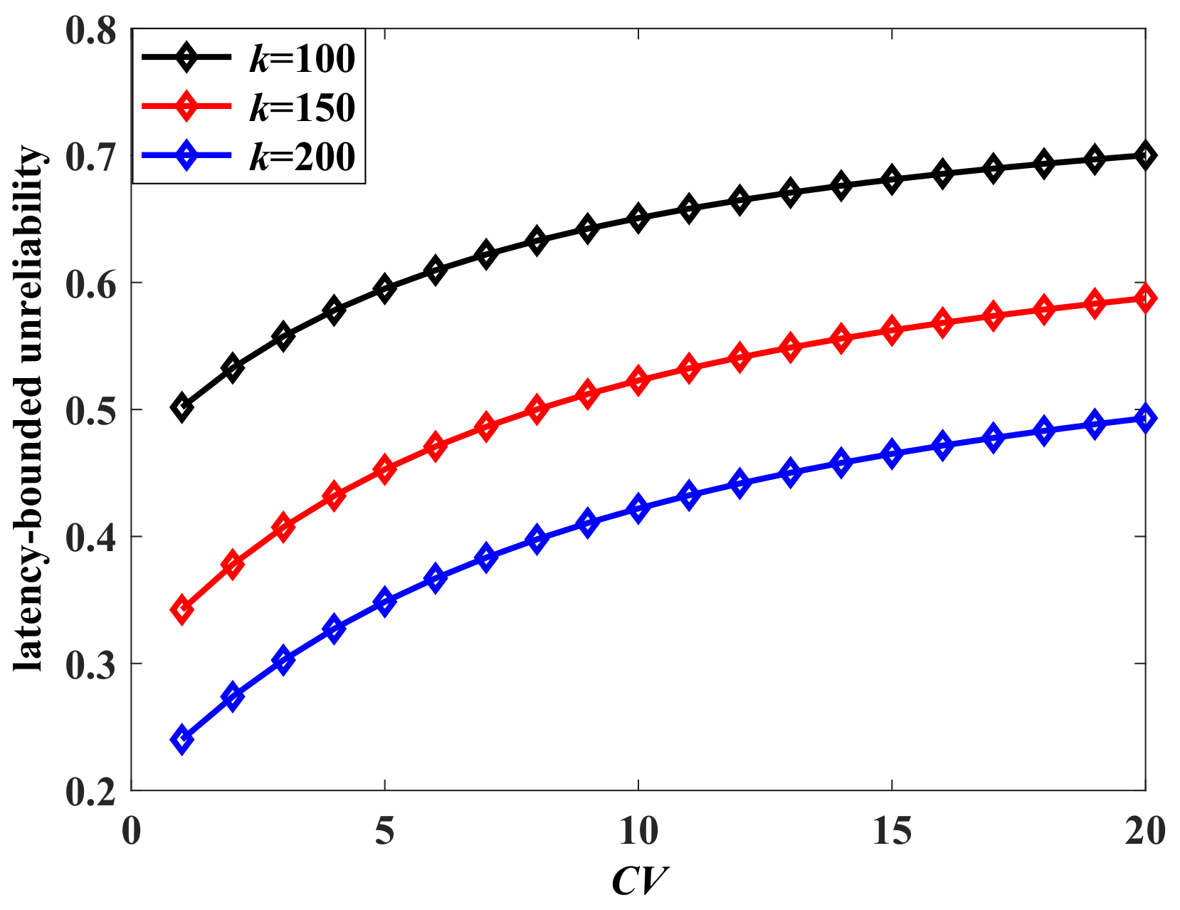
Next, we analyze the impact of the burstiness of the aggregate traffic on the latency-bounded unreliability. Two measurement parameters of burstiness are adopted, which are the Hurst and squared coefficient of variation (
). We change the state transition probabilities of the arrival models to influence the burstiness of aggregate traffic. The Hurst parameter is computed by the method of rescaled adjusted range analysis in this paper. Corresponding to the adjusted state transition probabilities (
), the Hurst parameter is
, respectively. The
of MMMP-4 can be derived as in (
24), where
is the average rate of the MMMP-4 model. A larger Hurst parameter or
indicates a stronger burstiness of the traffic. The latency-bounded unreliability versus latency threshold with different Hurst parameters is shown in
Figure 5, and the unreliability versus
is in
Figure 6. In
Figure 5 and
Figure 6, the system loads are
and
, respectively, which are relatively high. The latency performance decreases sharply with the burstiness. The system will become unsustainable when the system load is high along with a bursty arrival. With the
rising from 5 to 20, the system could only provide a best-effort QoS in the current service configuration. For the aggregate traffic with complex stochastic features, the impacts of burstiness on the latency-bounded reliability must be considered.
Finally, the impacts of system load on the latency performance are analyzed.
Figure 7 presents the results of latency-bounded unreliability versus
of the aggregate traffic,
. When
packets/slot, the system load is lower than
. If the threshold
k is relatively loose, the latency-bounded reliability is acceptable. However, for the business with strict latency threshold requirements (
to 70), the unreliability increases linearly with the system load. System load is an essential factor impacting the latency performance. If the system load goes too high, latency performance is unsatisfactory even if the latency threshold is moderate and the average arrival is not too large. From another perspective, even if the load is not high, the strong burstiness of arrivals may cause latency thresholds (those relatively small) to be violated frequently. The dotted lines in
Figure 7 support our analysis.
- B.
Relay selection algorithm performance
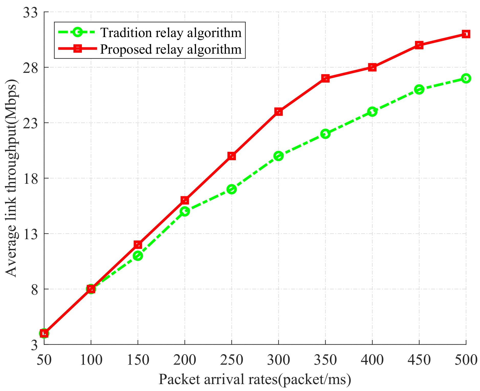
We compare two relay selection algorithms: (1) our proposed relay selection algorithm based on the back-pressure theory, and (2) the traditional relay selection algorithm based on the max–min criterion method. In
Figure 8, we show the evaluation of two relay selection algorithms through the average link throughput. From the figure, we can find that the average link throughput continues to increase with the increasing packet arrival rate, under two relay selection algorithms. Our proposed relay selection algorithm always achieves higher throughput than the traditional relay selection algorithm. It shows that the back-pressure theory can alleviate bandwidth limitations.
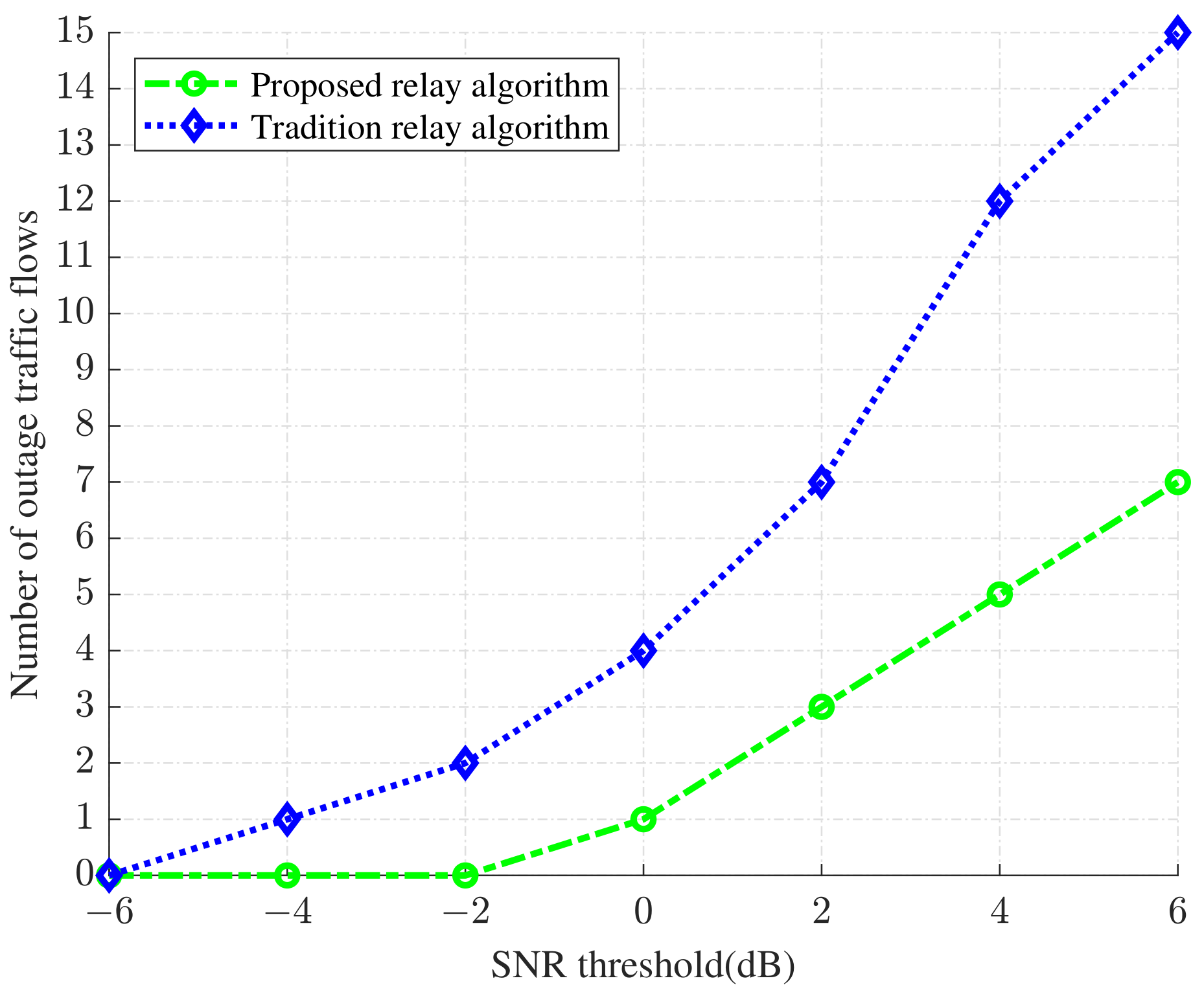
In
Figure 9, we plot the relationship between the signal-to-noise ratio (SNR) threshold and outage traffic flows, under traditional and our proposed relay selection algorithm. If the SNR is still lower than the SNR threshold after the relay selection algorithm optimization, the transmission channel will be interrupted, i.e., outage traffic flows are interrupted. From the figure, we find that when the SNR threshold increases, both relay selection algorithms increase the number of outage traffic flows. However, the number of outage traffic flows from our proposed algorithm is significantly lower than that of the traditional algorithm. The result confirms that our proposed relay selection algorithm can provide better reliability network performance.


