

Prediction of Vertical Ground Reaction Forces Under Different Running Speeds: Integration of Wearable IMU with CNN-xLSTM


Abstract
:1. Introduction
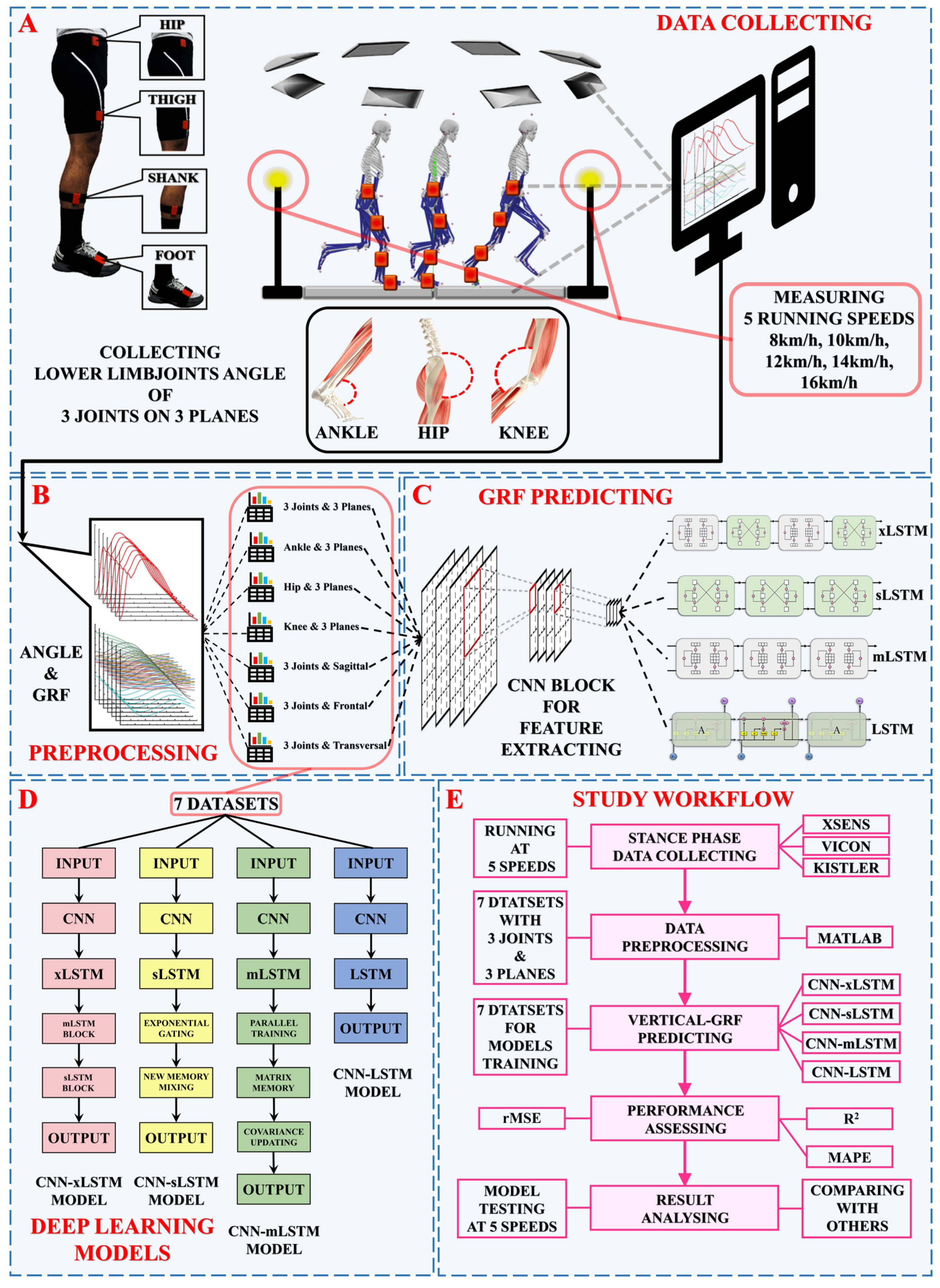
2. Procedure
2.1. Data Collection and Preprocessing
- 1.
- M1 (3Joints, 3Planes) = 530 × 909 (3joints × 3planes × 101angles);
- 2.
- M2 (Ankle, 3Planes) = 530 × 303 (1ankle joint × 3planes × 101angles);
- 3.
- M3 (Hip, 3Planes) = 530 × 303 (1hip joint × 3planes × 101angles);
- 4.
- M4 (Knee, 3Planes) = 530 × 303 (1knee joint × 3planes × 101angles);
- 5.
- M5 (3Joints, Sagittal) = 530 × 303 (3joints × 1sagittal plane × 101angles);
- 6.
- M6 (3Joints, Frontal) = 530 × 303 (3joints × 1frontal plane × 101angles);
- 7.
- M7 (3Joints, Transversal) = 530 × 303 (3joints × 1transversal plane × 101angles).
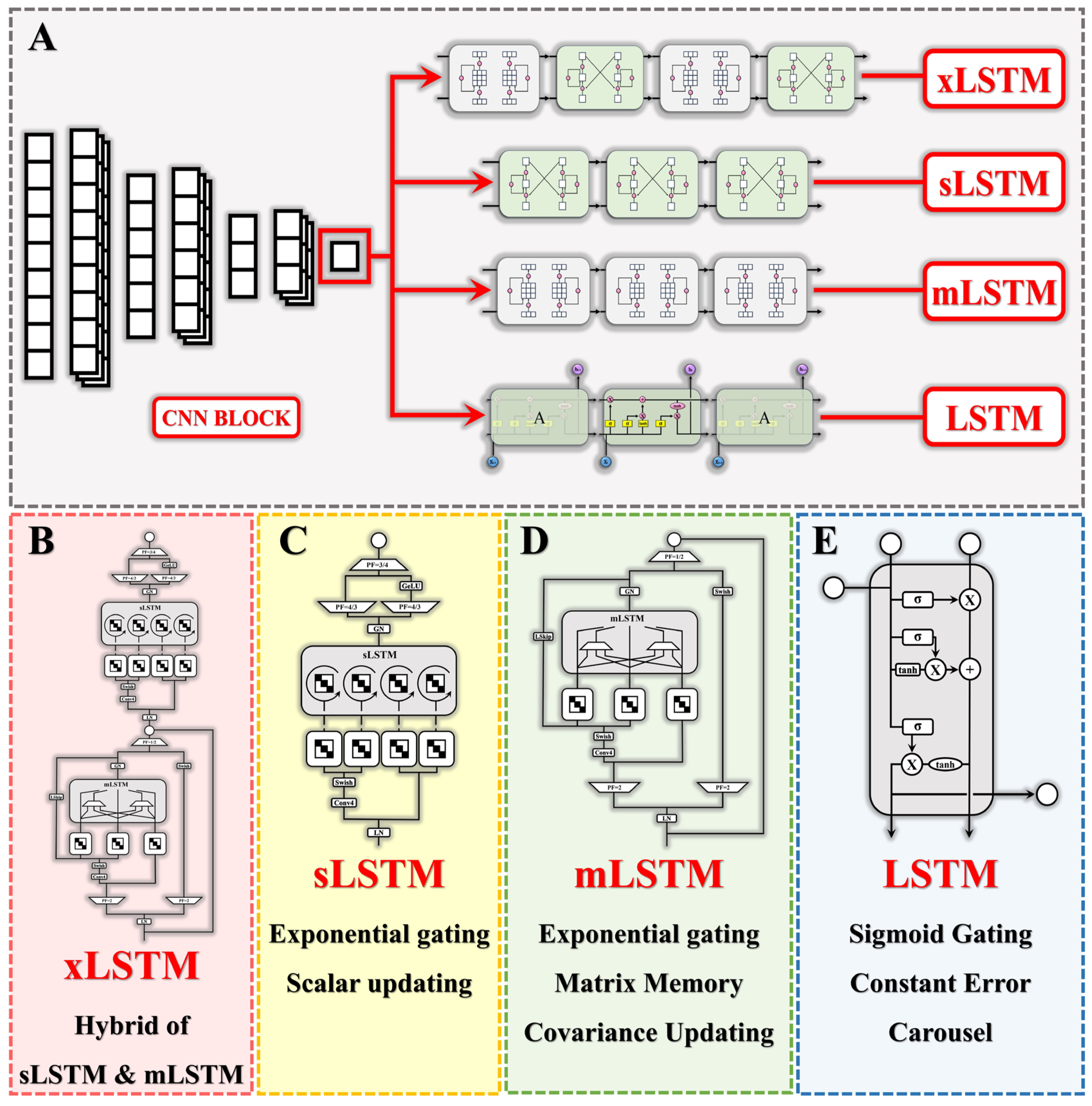
2.2. Deep Learning Models
2.2.1. Convolutional Neural Networks (CNNs)
2.2.2. Long Short-Term Memory (LSTM)
2.2.3. Extended Long Short-Term Memory (xLSTM)
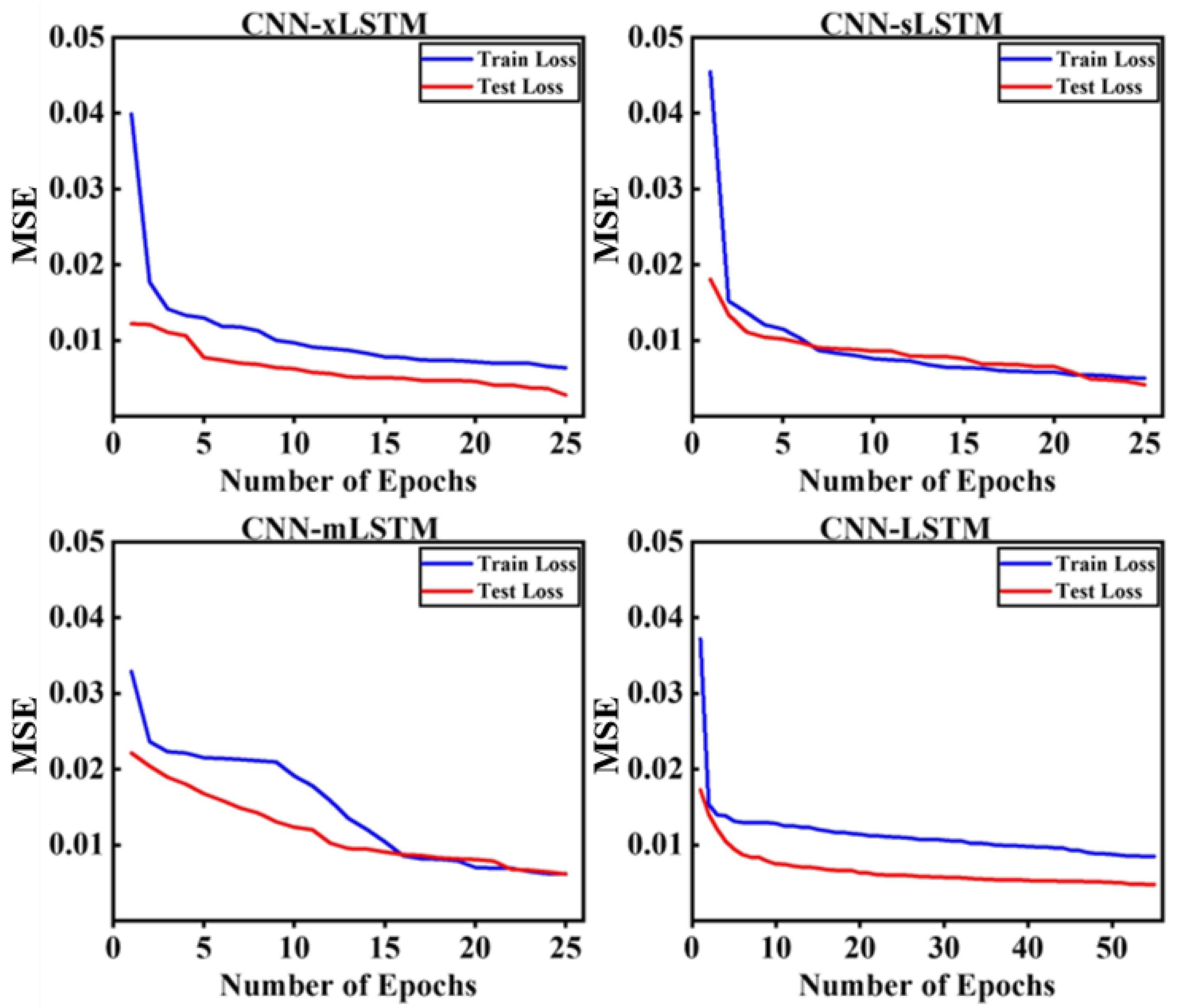
2.3. Model Training and Validation
2.3.1. Model Training
2.3.2. Model Validation
3. Results
3.1. Parameters of Deep Learning Models
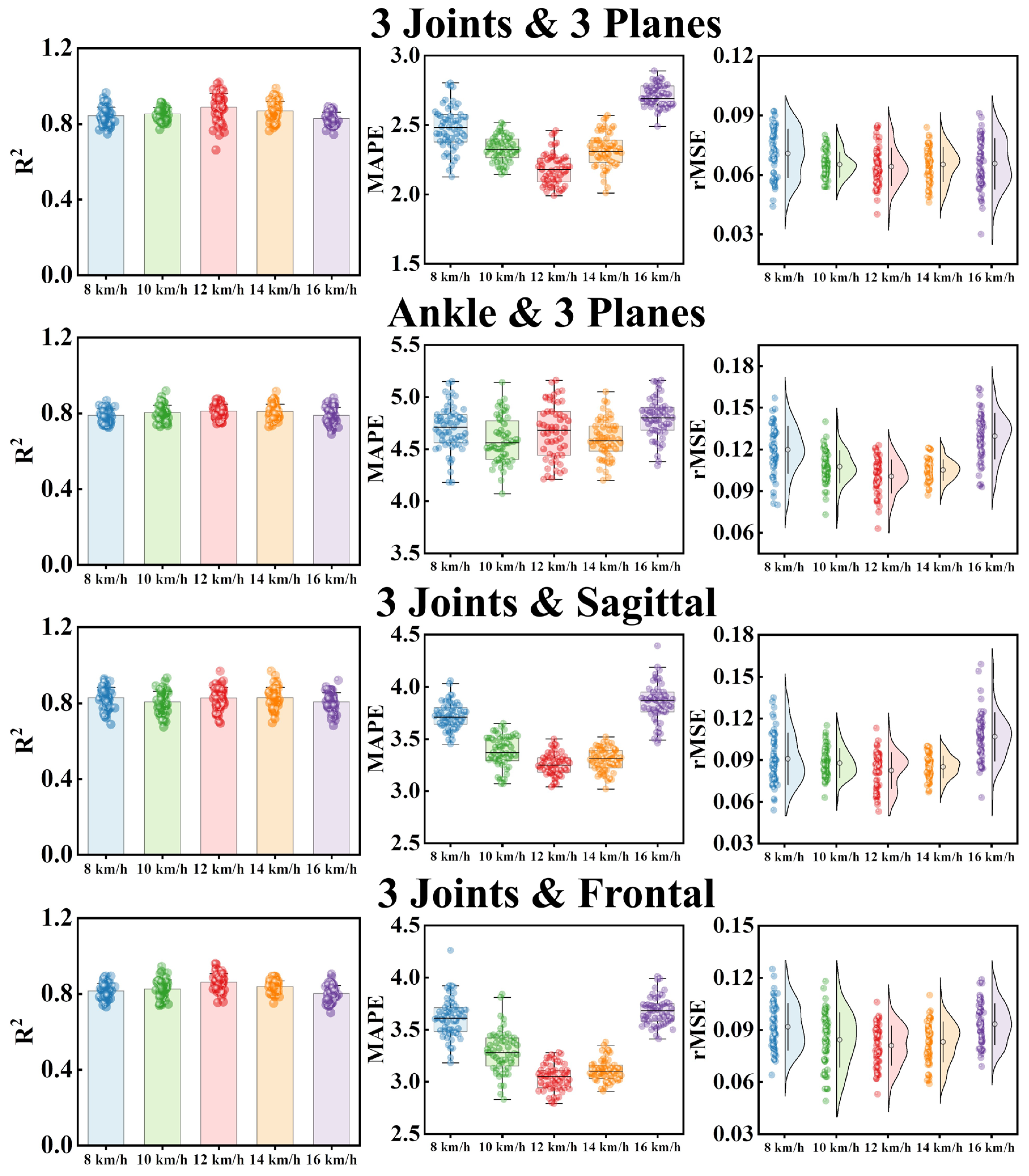
3.2. Prediction Results and Model Performance
3.3. Result Validation
4. Discussion
4.1. Contribution of Different Joint Angles
4.2. Performance of CNN-xLSTM
4.3. Prospects and Limitations
5. Conclusions
Author Contributions
Funding
Institutional Review Board Statement
Informed Consent Statement
Data Availability Statement
Conflicts of Interest
Abbreviations
| GRF | Ground Reaction Force |
| IMU | Inertial Measurement Unit |
| CNN | Convolutional Neural Network |
| LSTM | Long Short-Term Memory |
| xLSTM | Extended Long Short-Term Memory |
| sLSTM | Scalar Long Short-Term Memory |
| mLSTM | Matrix Long Short-Term Memory |
| R2 | Squared Correlation Coefficient |
| MAPE | Mean Absolute Percentage Error |
| rMSE | root Mean Squared Error |
References
- Van Oeveren, B.T.; de Ruiter, C.J.; Beek, P.J.; van Dieën, J.H. The biomechanics of running and running styles: A synthesis. Sports Biomech. 2024, 23, 516–554. [Google Scholar] [CrossRef] [PubMed]
- Souza, R.B. An evidence-based videotaped running biomechanics analysis. Phys. Med. Rehabil. Clin. 2016, 27, 217–236. [Google Scholar] [CrossRef] [PubMed]
- Leardini, A.; Benedetti, M.G.; Berti, L.; Bettinelli, D.; Nativo, R.; Giannini, S. Rear-foot, mid-foot and fore-foot motion during the stance phase of gait. Gait Posture 2007, 25, 453–462. [Google Scholar] [CrossRef] [PubMed]
- Van Hooren, B.; Bosch, F. Is there really an eccentric action of the hamstrings during the swing phase of high-speed running? Part I: A critical review of the literature. J. Sports Sci. 2017, 35, 2313–2321. [Google Scholar] [CrossRef]
- Zhou, H.; Ugbolue, U.C. Is there a relationship between strike pattern and injury during running: A review. Phys. Act. Health 2019, 3, 127–134. [Google Scholar] [CrossRef]
- Moore, I.S. Is there an economical running technique? A review of modifiable biomechanical factors affecting running economy. Sports Med. 2016, 46, 793–807. [Google Scholar] [CrossRef]
- Clark, K.P.; Ryan, L.J.; Weyand, P.G. Foot speed, foot-strike and footwear: Linking gait mechanics and running ground reaction forces. J. Exp. Biol. 2014, 217, 2037–2040. [Google Scholar]
- Yu, P.; Cen, X.; Mei, Q.; Wang, A.; Gu, Y.; Fernandez, J. Differences in intra-foot movement strategies during locomotive tasks among chronic ankle instability, copers and healthy individuals. J. Biomech. 2024, 162, 111865. [Google Scholar] [CrossRef]
- Gruber, A.H.; Edwards, W.B.; Hamill, J.; Derrick, T.R.; Boyer, K.A. A comparison of the ground reaction force frequency content during rearfoot and non-rearfoot running patterns. Gait Posture 2017, 56, 54–59. [Google Scholar] [CrossRef]
- Hall, J.P.; Barton, C.; Jones, P.R.; Morrissey, D. The biomechanical differences between barefoot and shod distance running: A systematic review and preliminary meta-analysis. Sports Med. 2013, 43, 1335–1353. [Google Scholar] [CrossRef]
- Tongen, A.; Wunderlich, R.E. Biomechanics of running and walking. Math. Sports 2010, 43, 315–327. [Google Scholar]
- Mizoguchi, M.; Calame, C. Possibilities and limitation of today’s force plate technology. Gait Posture 1995, 4, 268. [Google Scholar] [CrossRef]
- Oh, S.E.; Choi, A.; Mun, J.H. Prediction of ground reaction forces during gait based on kinematics and a neural network model. J. Biomech. 2013, 46, 2372–2380. [Google Scholar] [CrossRef] [PubMed]
- Fluit, R.; Andersen, M.S.; Kolk, S.; Verdonschot, N.; Koopman, H.F. Prediction of ground reaction forces and moments during various activities of daily living. J. Biomech. 2014, 47, 2321–2329. [Google Scholar] [CrossRef] [PubMed]
- Xu, D.; Zhou, H.; Quan, W.; Gusztav, F.; Baker, J.S.; Gu, Y. Adaptive neuro-fuzzy inference system model driven by the non-negative matrix factorization-extracted muscle synergy patterns to estimate lower limb joint movements. Comput. Methods Programs Biomed. 2023, 242, 107848. [Google Scholar] [CrossRef]
- Chaaban, C.R.; Berry, N.T.; Armitano-Lago, C.; Kiefer, A.W.; Mazzoleni, M.J.; Padua, D.A. Combining inertial sensors and machine learning to predict vGRF and knee biomechanics during a double limb jump landing task. Sensors 2021, 21, 4383. [Google Scholar] [CrossRef]
- Greenhalgh, A.; Sinclair, J.; Protheroe, L.; Chockalingam, N. Predicting impact shock magnitude: Which ground reaction force variable should we use. Int. J. Sports Sci. Eng. 2012, 6, 225–231. [Google Scholar]
- Johnson, C.D.; Tenforde, A.S.; Outerleys, J.; Reilly, J.; Davis, I.S. Impact-related ground reaction forces are more strongly associated with some running injuries than others. Am. J. Sports Med. 2020, 48, 3072–3080. [Google Scholar] [CrossRef]
- Xu, D.; Quan, W.; Zhou, H.; Sun, D.; Baker, J.S.; Gu, Y. Explaining the differences of gait patterns between high and low-mileage runners with machine learning. Sci. Rep. 2022, 12, 2981. [Google Scholar] [CrossRef]
- Xu, D.; Zhou, H.; Quan, W.; Gusztav, F.; Wang, M.; Baker, J.S.; Gu, Y. Accurately and effectively predict the ACL force: Utilizing biomechanical landing pattern before and after-fatigue. Comput. Methods Programs Biomed. 2023, 241, 107761. [Google Scholar] [CrossRef]
- Xu, D.; Zhou, H.; Quan, W.; Jiang, X.; Liang, M.; Li, S.; Ugbolue, U.C.; Baker, J.S.; Gusztav, F.; Ma, X. A new method proposed for realizing human gait pattern recognition: Inspirations for the application of sports and clinical gait analysis. Gait Posture 2024, 107, 293–305. [Google Scholar] [CrossRef] [PubMed]
- Xu, D.; Zhou, H.; Quan, W.; Ma, X.; Chon, T.-E.; Fernandez, J.; Gusztav, F.; Kovács, A.; Baker, J.S.; Gu, Y. New insights optimize landing strategies to reduce lower limb injury risk. Cyborg Bionic Syst. 2024, 5, 0126. [Google Scholar] [CrossRef] [PubMed]
- Halilaj, E.; Rajagopal, A.; Fiterau, M.; Hicks, J.L.; Hastie, T.J.; Delp, S.L. Machine learning in human movement biomechanics: Best practices, common pitfalls, and new opportunities. J. Biomech. 2018, 81, 1–11. [Google Scholar] [CrossRef] [PubMed]
- Scheltinga, B.L.; Kok, J.N.; Buurke, J.H.; Reenalda, J. Estimating 3D ground reaction forces in running using three inertial measurement units. Front. Sports Act. Living 2023, 5, 1176466. [Google Scholar] [CrossRef]
- Pogson, M.; Verheul, J.; Robinson, M.A.; Vanrenterghem, J.; Lisboa, P. A neural network method to predict task-and step-specific ground reaction force magnitudes from trunk accelerations during running activities. Med. Eng. Phys. 2020, 78, 82–89. [Google Scholar] [CrossRef]
- Bogaert, S.; Davis, J.; Vanwanseele, B. Predicting vertical ground reaction force characteristics during running with machine learning. Front. Bioeng. Biotechnol. 2024, 12, 1440033. [Google Scholar] [CrossRef]
- Du, X.; Vasudevan, R.; Johnson-Roberson, M. Bio-lstm: A biomechanically inspired recurrent neural network for 3-d pedestrian pose and gait prediction. IEEE Robot. Autom. Lett. 2019, 4, 1501–1508. [Google Scholar] [CrossRef]
- Gers, F.A.; Schmidhuber, J.; Cummins, F. Learning to forget: Continual prediction with LSTM. Neural Comput. 2000, 12, 2451–2471. [Google Scholar] [CrossRef]
- Alcantara, R.S.; Edwards, W.B.; Millet, G.Y.; Grabowski, A.M. Predicting continuous ground reaction forces from accelerometers during uphill and downhill running: A recurrent neural network solution. PeerJ 2022, 10, e12752. [Google Scholar] [CrossRef]
- Donahue, S.R.; Hahn, M.E. Estimation of ground reaction force waveforms during fixed pace running outside the laboratory. Front. Sports Act. Living 2023, 5, 974186. [Google Scholar] [CrossRef]
- Beck, M.; Pöppel, K.; Spanring, M.; Auer, A.; Prudnikova, O.; Kopp, M.; Klambauer, G.; Brandstetter, J.; Hochreiter, S. xLSTM: Extended Long Short-Term Memory. arXiv 2024, arXiv:2405.04517. [Google Scholar]
- Alkin, B.; Beck, M.; Pöppel, K.; Hochreiter, S.; Brandstetter, J. Vision-LSTM: xLSTM as Generic Vision Backbone. arXiv 2024, arXiv:2406.04303. [Google Scholar]
- Alharthi, M.; Mahmood, A. xlstmtime: Long-term time series forecasting with xlstm. AI 2024, 5, 1482–1495. [Google Scholar] [CrossRef]
- Chen, T.; Ding, C.; Zhu, L.; Xu, T.; Yan, W.; Ji, D.; Li, Z.; Zang, Y. xLSTM-UNet can be an Effective Backbone for 2D & 3D Biomedical Image Segmentation Better than its Mamba Counterparts. In Proceedings of the IEEE-EMBS International Conference on Biomedical and Health Informatics, Houston, TX, USA, 10–13 November 2024. [Google Scholar]
- Fan, X.; Tao, C.; Zhao, J. Advanced stock price prediction with xlstm-based models: Improving long-term forecasting. In Proceedings of the 2024 11th International Conference on Soft Computing & Machine Intelligence (ISCMI), Melbourne, Australia, 22–23 November 2024. [Google Scholar]
- Wang, W.; Lian, C.; Zhao, Y.; Zhan, Z. Sensor-Based Gymnastics Action Recognition Using Time-Series Images and a Lightweight Feature Fusion Network. IEEE Sens. J. 2024, 24, 42573–42583. [Google Scholar] [CrossRef]
- Giarmatzis, G.; Zacharaki, E.I.; Moustakas, K. Real-time prediction of joint forces by motion capture and machine learning. Sensors 2020, 20, 6933. [Google Scholar] [CrossRef]
- Stetter, B.J.; Ringhof, S.; Krafft, F.C.; Sell, S.; Stein, T. Estimation of knee joint forces in sport movements using wearable sensors and machine learning. Sensors 2019, 19, 3690. [Google Scholar] [CrossRef]
- Wang, Z.; Qiu, Q.; Chen, S.; Chen, B.; Lv, X. Effects of unstable shoes on lower limbs with different speeds. Phys. Act. Health 2019, 3, 82–88. [Google Scholar] [CrossRef]
- De Wit, B.; De Clercq, D.; Aerts, P. Biomechanical analysis of the stance phase during barefoot and shod running. J. Biomech. 2000, 33, 269–278. [Google Scholar] [CrossRef]
- Alzubaidi, L.; Zhang, J.; Humaidi, A.J.; Al-Dujaili, A.; Duan, Y.; Al-Shamma, O.; Santamaría, J.; Fadhel, M.A.; Al-Amidie, M.; Farhan, L. Review of deep learning: Concepts, CNN architectures, challenges, applications, future directions. J. Big Data 2021, 8, 53. [Google Scholar] [CrossRef]
- Liu, Y.; Fernandez, J. Randomized Controlled Trial of Gastrocnemius Muscle Analysis Using Surface Electromyography and Ultrasound in Different Striking Patterns of Young Women’s Barefoot Running. Phys. Act. Health 2024, 8, 223–233. [Google Scholar] [CrossRef]
- Chang, H.; Cen, X. Can running technique modification benefit patellofemoral pain improvement in runners? A systematic review and meta-analysis. Int. J. Biomed. Eng. Technol. 2024, 45, 83–101. [Google Scholar] [CrossRef]
- Xu, D.; Lu, J.; Baker, J.S.; Fekete, G.; Gu, Y. Temporal kinematic and kinetics differences throughout different landing ways following volleyball spike shots. Proc. Inst. Mech. Eng. Part P 2022, 236, 200–208. [Google Scholar] [CrossRef]
- Fang, Z.; Shi, K.; Han, Q. When Mamba Meets xLSTM: An Efficient and Precise Method with the XLSTM-VMUNet Model for Skin lesion Segmentation. arXiv 2024, arXiv:2411.09363. [Google Scholar]
- Zhu, Q.; Cai, Y.; Fan, L. Seg-LSTM: Performance of xLSTM for Semantic Segmentation of Remotely Sensed Images. arXiv 2024, arXiv:2406.14086. [Google Scholar]


| Model | Batch Size | Hidden Size | Epochs | Stacked Layers | Module |
|---|---|---|---|---|---|
| CNN-xLSTM | 128 | 64 | 25 | 1 | ‘m’, ’s’ |
| CNN-sLSTM | 128 | 64 | 25 | 1 | ‘s’ |
| CNN-mLSTM | 128 | 64 | 25 | 1 | ‘m’ |
| CNN-LSTM | 256 | 128 | 55 | 2 | / |
| Models | Index | M1 | M2 | M3 | M4 | M5 | M6 | M7 |
|---|---|---|---|---|---|---|---|---|
| CNN-xLSTM | R2 | 0.909 ± 0.064 | 0.814 ± 0.053 | 0.757 ± 0.092 | 0.709 ± 0.074 | 0.836 ± 0.042 | 0.861 ± 0.057 | 0.671 ± 0.051 |
| MAPE | 2.18 ± 0.09 | 4.38 ± 0.21 | 9.95 ± 0.34 | 10.01 ± 0.41 | 3.17 ± 0.12 | 3.09 ± 0.18 | 12.82 ± 0.33 | |
| rMSE | 0.061 ± 0.008 | 0.089 ± 0.010 | 0.119 ± 0.014 | 0.132 ± 0.021 | 0.074 ± 0.007 | 0.070 ± 0.006 | 0.138 ± 0.017 | |
| CNN-sLSTM | R2 | 0.748 ± 0.056 | 0.702 ± 0.044 | 0.622 ± 0.069 | 0.656 ± 0.046 | 0.711 ± 0.055 | 0.729 ± 0.073 | 0.491 ± 0.067 |
| MAPE | 3.71 ± 0.32 | 6.74 ± 0.59 | 17.06 ± 0.60 | 13.88 ± 0.77 | 6.27 ± 0.47 | 5.78 ± 0.58 | 15.06 ± 0.76 | |
| rMSE | 0.097 ± 0.011 | 0.114 ± 0.009 | 0.143 ± 0.014 | 0.161 ± 0.023 | 0.092 ± 0.007 | 0.094 ± 0.005 | 0.168 ± 0.028 | |
| CNN-mLSTM | R2 | 0.791 ± 0.027 | 0.713 ± 0.031 | 0.608 ± 0.035 | 0.627 ± 0.025 | 0.709 ± 0.031 | 0.721 ± 0.027 | 0.626 ± 0.031 |
| MAPE | 5.56 ± 0.38 | 8.58 ± 1.04 | 19.49 ± 1.13 | 17.39 ± 0.93 | 9.19 ± 0.72 | 10.20 ± 0.97 | 16.38 ± 1.45 | |
| rMSE | 0.092 ± 0.012 | 0.112 ± 0.013 | 0.178 ± 0.032 | 0.209 ± 0.014 | 0.093 ± 0.013 | 0.096 ± 0.008 | 0.158 ± 0.024 | |
| CNN-LSTM | R2 | 0.742 ± 0.040 | 0.683 ± 0.032 | 0.619 ± 0.034 | 0.628 ± 0.041 | 0.728 ± 0.039 | 0.717 ± 0.041 | 0.653 ± 0.042 |
| MAPE | 7.17 ± 0.45 | 8.12 ± 0.53 | 14.44 ± 1.05 | 15.07 ± 1.50 | 8.50 ± 0.80 | 8.89 ± 0.49 | 13.54 ± 0.98 | |
| rMSE | 0.104 ± 0.018 | 0.108 ± 0.006 | 0.135 ± 0.029 | 0.173 ± 0.037 | 0.112 ± 0.010 | 0.105 ± 0.008 | 0.172 ± 0.015 |
| Inputs | Index | 8 km/h | 10 km/h | 12 km/h | 14 km/h | 16 km/h |
|---|---|---|---|---|---|---|
| 3 Joints and 3 Planes | R2 | 0.842 ± 0.047 | 0.854 ± 0.043 | 0.879 ± 0.068 | 0.861 ± 0.054 | 0.836 ± 0.032 |
| MAPE | 2.45 ± 0.18 | 2.33 ± 0.09 | 2.19 ± 0.12 | 2.36 ± 0.11 | 2.71 ± 0.08 | |
| rMSE | 0.069 ± 0.012 | 0.067 ± 0.007 | 0.063 ± 0.010 | 0.065 ± 0.009 | 0.070 ± 0.013 | |
| Ankle and 3 Planes | R2 | 0.801 ± 0.037 | 0.804 ± 0.039 | 0.811 ± 0.036 | 0.807 ± 0.044 | 0.793 ± 0.043 |
| MAPE | 4.69 ± 0.22 | 4.63 ± 0.26 | 4.45 ± 0.19 | 4.59 ± 0.18 | 4.78 ± 0.20 | |
| rMSE | 0.116 ± 0.018 | 0.109 ± 0.013 | 0.101 ± 0.011 | 0.105 ± 0.009 | 0.127 ± 0.021 | |
| 3 Joints and Sagittal | R2 | 0.819 ± 0.62 | 0.821 ± 0.058 | 0.831 ± 0.055 | 0.829 ± 0.060 | 0.813 ± 0.052 |
| MAPE | 3.73 ± 0.13 | 3.39 ± 0.15 | 3.24 ± 0.11 | 3.29 ± 0.12 | 3.87 ± 0.17 | |
| rMSE | 0.093 ± 0.019 | 0.089 ± 0.011 | 0.082 ± 0.012 | 0.085 ± 0.010 | 0.104 ± 0.014 | |
| 3 Joints and Frontal | R2 | 0.811 ± 0.038 | 0.832 ± 0.050 | 0.857 ± 0.043 | 0.841 ± 0.037 | 0.803 ± 0.046 |
| MAPE | 3.65 ± 0.21 | 3.27 ± 0.19 | 3.06 ± 0.13 | 3.12 ± 0.11 | 3.71 ± 0.16 | |
| rMSE | 0.091 ± 0.013 | 0.085 ± 0.017 | 0.079 ± 0.012 | 0.082 ± 0.012 | 0.093 ± 0.011 |
| Studies | Models | Inputs | R2 | MAPE (%) | rMSE |
|---|---|---|---|---|---|
| Oh et al. (2013) [13] | ANN | Centre of Mass and Acceleration of Segments and Joints | 0.982 | / | 0.058 ± 0.010 |
| Pogson et al. (2020) [25] | PCA-MLP-ANN | Trunk Acceleration | 0.900 | / | / |
| Alcantara et al. (2022) [29] | LSTM | Height, Mass, Speed, Slope, and Running Pattern | / | / | 0.064 ± 0.015 |
| Scheltinga et al. (2023) [24] | ensANN | Acceleration of Pelvis and Tibias | 0.960 | / | 0.066 ± 0.001 |
| Bogaert et al. (2024) [26] | Lasso | 3-Dimensional Sacral Acceleration | 0.870 | 3.29 | 0.106 |
| Donahue et al. (2023) [30] | LSTM | 3D accelerations and angular velocities | / | / | 0.189 |
| This Study | CNN-xLSTM | Joints Angle of Ankle, Hip, and Knee | 0.973 | 2.18 ± 0.09 | 0.061 ± 0.008 |
Disclaimer/Publisher’s Note: The statements, opinions and data contained in all publications are solely those of the individual author(s) and contributor(s) and not of MDPI and/or the editor(s). MDPI and/or the editor(s) disclaim responsibility for any injury to people or property resulting from any ideas, methods, instructions or products referred to in the content. |
© 2025 by the authors. Licensee MDPI, Basel, Switzerland. This article is an open access article distributed under the terms and conditions of the Creative Commons Attribution (CC BY) license (https://creativecommons.org/licenses/by/4.0/).
Share and Cite
Chen, T.; Xu, D.; Zhou, Z.; Zhou, H.; Shao, S.; Gu, Y. Prediction of Vertical Ground Reaction Forces Under Different Running Speeds: Integration of Wearable IMU with CNN-xLSTM. Sensors 2025, 25, 1249. https://doi.org/10.3390/s25041249
Chen T, Xu D, Zhou Z, Zhou H, Shao S, Gu Y. Prediction of Vertical Ground Reaction Forces Under Different Running Speeds: Integration of Wearable IMU with CNN-xLSTM. Sensors. 2025; 25(4):1249. https://doi.org/10.3390/s25041249
Chicago/Turabian StyleChen, Tianxiao, Datao Xu, Zhifeng Zhou, Huiyu Zhou, Shirui Shao, and Yaodong Gu. 2025. "Prediction of Vertical Ground Reaction Forces Under Different Running Speeds: Integration of Wearable IMU with CNN-xLSTM" Sensors 25, no. 4: 1249. https://doi.org/10.3390/s25041249
APA StyleChen, T., Xu, D., Zhou, Z., Zhou, H., Shao, S., & Gu, Y. (2025). Prediction of Vertical Ground Reaction Forces Under Different Running Speeds: Integration of Wearable IMU with CNN-xLSTM. Sensors, 25(4), 1249. https://doi.org/10.3390/s25041249