
Deep Learning Based Pile-Up Correction Algorithm for Spectrometric Data Under High-Count-Rate Measurements

 , , , , and
Abstract
1. Introduction
- Spectrum Estimation Model for High Count Rates: A novel model is proposed for pile-up correction and spectrum estimation for high-count-rate scenarios. It achieves accurate predictions even in heavily distorted conditions, addressing the challenges in high-activity gamma source analysis;
- Innovative Input Design with Energy–Duration Matrix: The Energy–Duration matrix, constructed via zero-crossing segmentation, is introduced as the input for 2D-UNet. This design effectively represents the mandatory information for pile-up correction;
- Hybrid Model Combining Temporal and Spatial Features: This work integrates activity information and 2D-UNet architectures to extract temporal dependencies and spatial features from pulse signals. The embedding of count rate information enhances the robustness and accuracy of spectrum recovery under high count rate conditions.
2. Problem Formulation
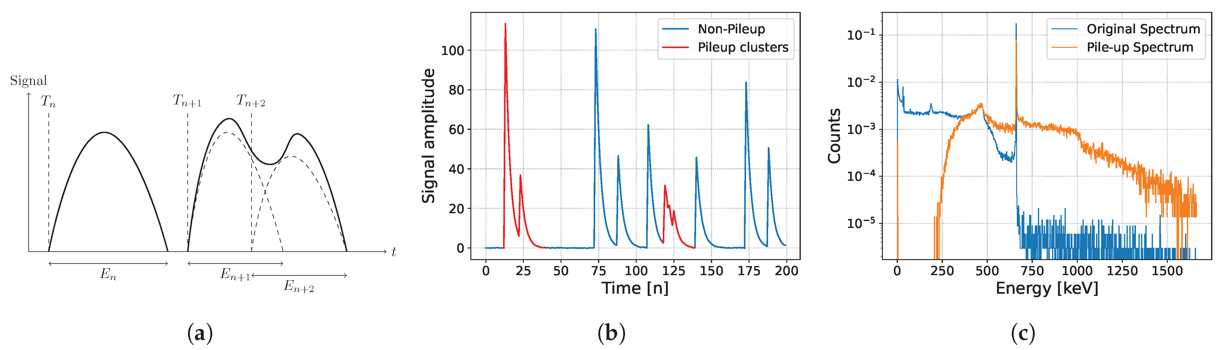
2.1. Pile-Up Description and Correction Theory
2.2. Signal Formula
- Shape dictionary: One of the common shape models is the double exponential [1] which can be modeled as:where a is the normalization factor and are characteristic decay times. For practical purposes, any pulse shape is assumed to have a finite time length . A key characteristic of the pulse shape is the peak time, , also known as the rise time, which is complementary to the fall time . For instance, the rise time for the double exponential model is given by:where are the decay times. In practice, a single precise parameter set cannot perfectly fit the pulse shape due to the physical inhomogeneities, temperature fluctuation, and other factors, leading us to generate our parameter set randomly from a Gaussian distribution with reasonable expectations and variances [22].
- Arrival times: as mentioned above, the arrival of gamma particles is modeled using a Poisson counting process with a constant intensity of . The inter-arrival times follow an exponential distribution with expectation .
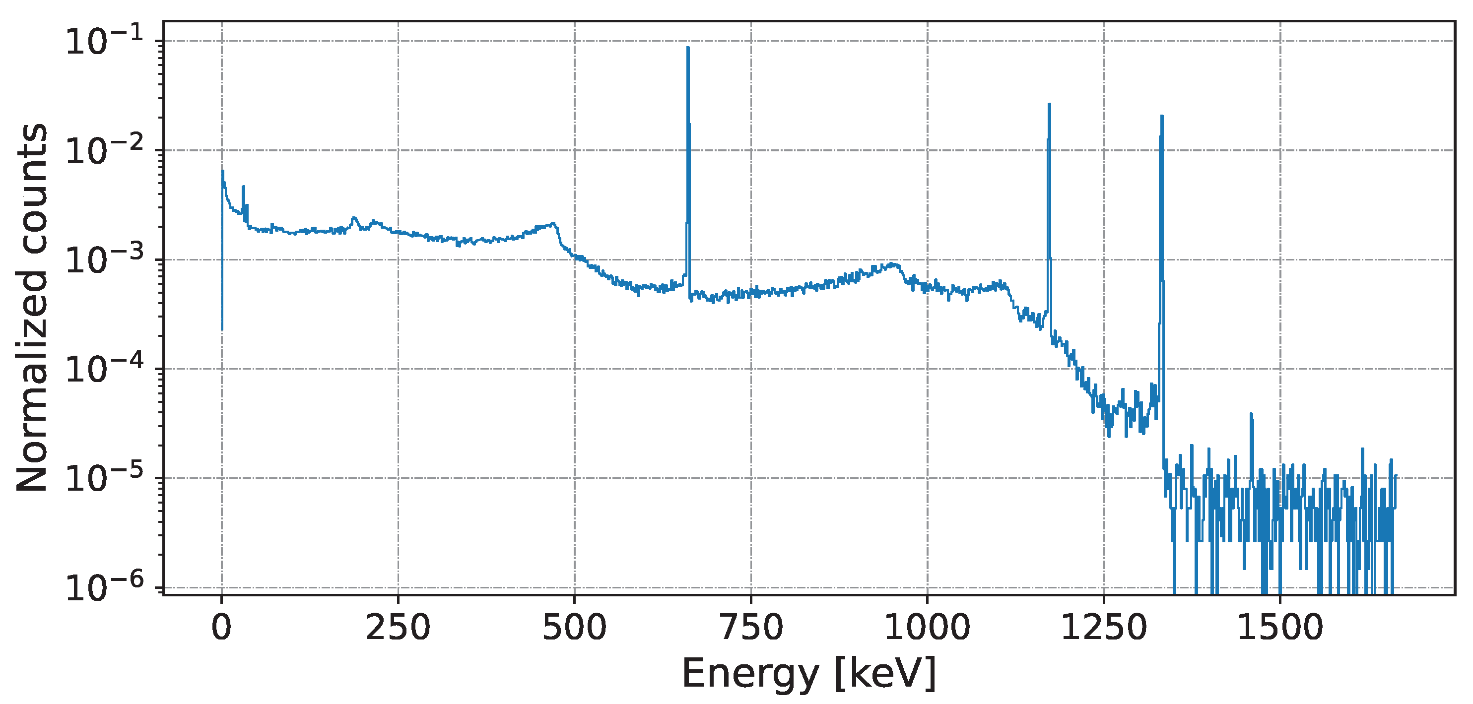
- Source: The spectrum of the signal can be either single source or multi-sources, the interactions among a mixture of multiple elements can be formed as:where represents the probability that emits energy e, E is the signal source’s spectrum, and is the proportion of source . Thus, the spectrum of the mixture sources can be modeled as the following:By doing so, the probability density function of the mixture histogram can be derived.
- Energy–Probability: The common representation of the probability of arrival particles’ energies per energy bin (typically measured by keV) is by a histogram that represents the energies of a series of signal events. This energy histogram can be easily modeled by a discrete random distribution where the probability of energy is proportional to :where is the number of events with energy, B represents the bin index, and the pairs of values for and of a single source or mixed source can be determined by the accept–reject method [23]. An example of a mixed spectrum is shown in Figure 2.
2.3. Dataset Generation
2.4. Pulse Signal Segmentation
2.5. Energy–Duration Matrix Construction
3. Method
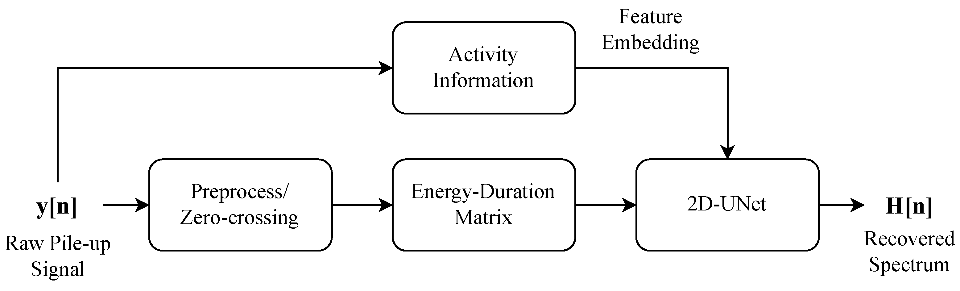
- Pulse Signal Preprocessing: The raw pulse signals are first processed to generate an Energy–Duration matrix, which is achieved by segmenting the signal based on zero-crossing points. The resulting Energy–Duration matrix contains the spatial characteristics of the signal and serves as a feature representation for the 2D U-Net model.
- Embedding Count Rate Information into 2D U-Net: The true count rate information is directly embedded into the 2D U-Net model, representing the temporal feature, intuitively giving the model prior information about the intensity of signal pile-up. This allows the 2D U-Net to process both spatial and temporal features simultaneously.
- Energy Spectrum Recovery: The 2D U-Net, now augmented with the Energy–Duration matrix and the count rate information, processes these inputs to generate the predicted energy spectrum. The output of the network is compared with the true energy spectrum during training, and the model is optimized to minimize the reconstruction error using Mean Squared Error (MSE).
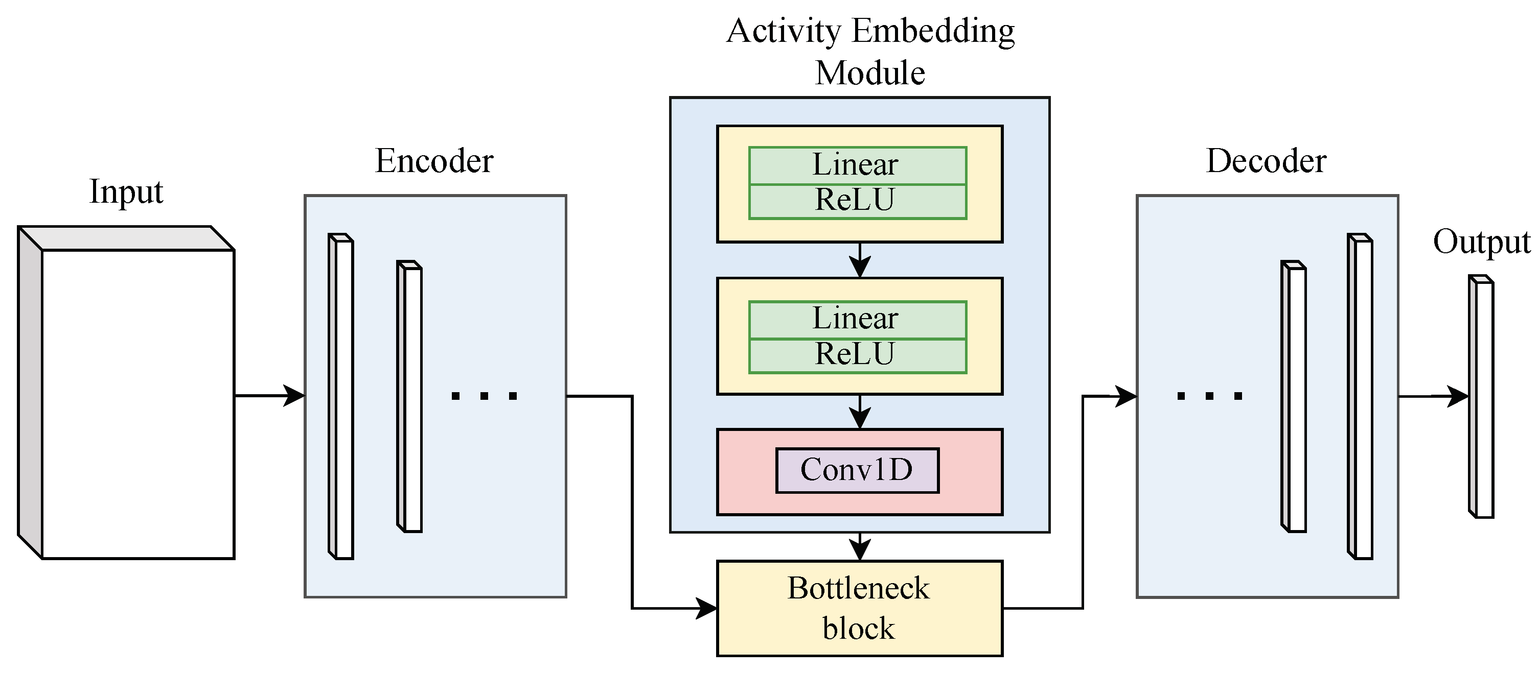
3.1. Count Rate Embedding Module
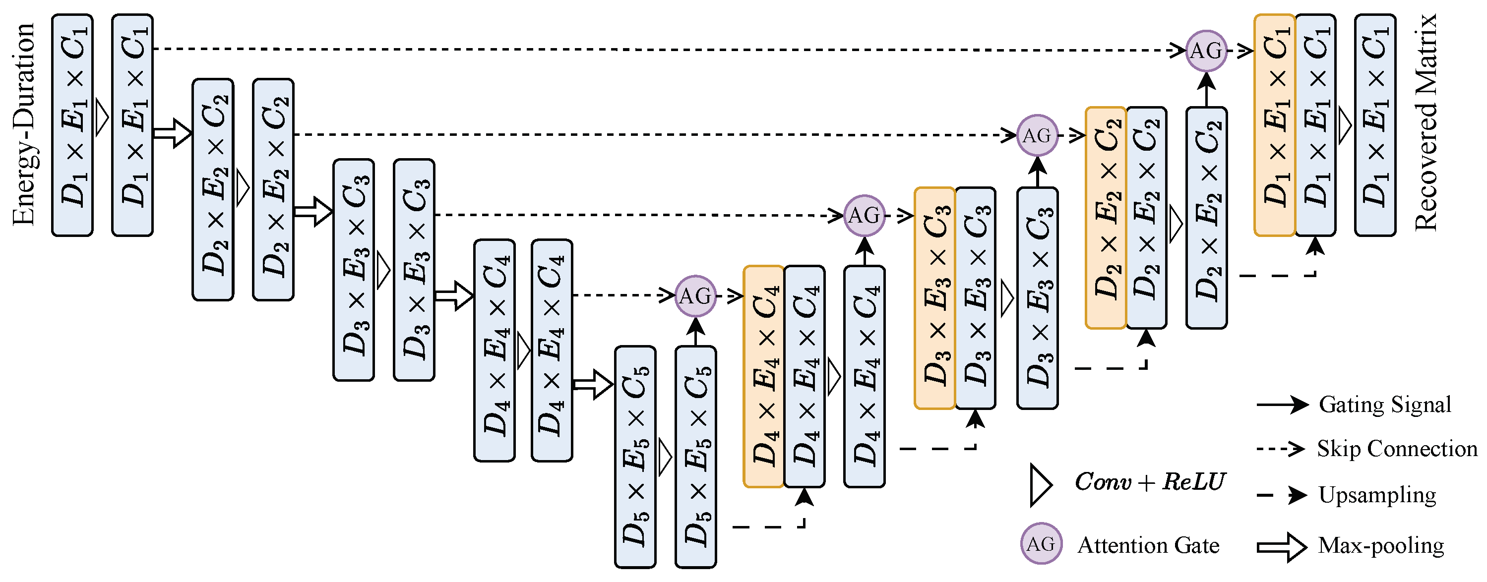
3.2. 2D-UNet
3.2.1. Attention U-Net Model Architecture
3.2.2. Encoder Architecture
3.2.3. Decoder Architecture
3.2.4. Attention Gates
3.2.5. Final Output Layer
3.3. Loss Function and Optimization
4. Experiments
4.1. Training Parameters
4.2. Hardware and Software Setup
4.3. Evaluation Metrics
- Method 1: A baseline method that does not correct for pulse pile-up.
- Method 2: A fast correction algorithm, as described in [21].
5. Results and Discussion
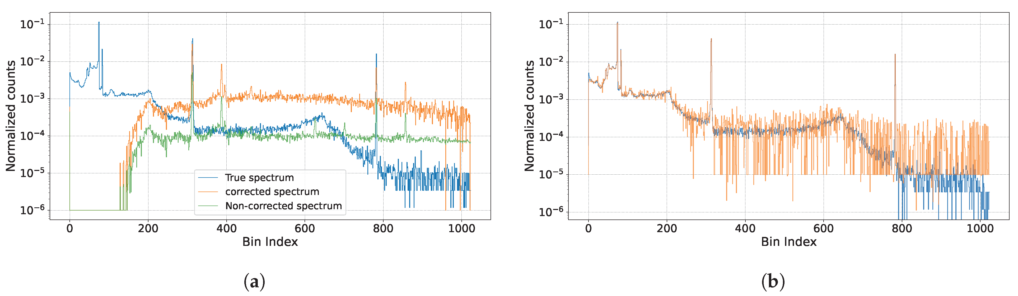
5.1. Visualization
- In low pile-up conditions (e.g., Figure 6a, ), the estimated peaks closely align with the ground truth spectrum, showcasing minimal deviations.
- As the pile-up level increases (e.g., Figure 6f, ), slight deviations are observed, particularly in higher-energy regions. Nevertheless, the primary peaks remain well-estimated, and the overall spectral trends are preserved.
- Across all cases, the proposed method effectively reconstructs the peaks, even under severe pile-up conditions, highlighting its robustness and accuracy.
5.2. Quantification
6. Conclusions
Author Contributions
Funding
Data Availability Statement
Conflicts of Interest
References
- Knoll, G.F. Radiation Detection and Measurement, 4th ed.; Wiley: Hoboken, NJ, USA, 2010. [Google Scholar]
- Siddavatam, A.P.I.; Vaidya, P.P.; Nair, J.M. Pileup rejection using estimation technique for high resolution nuclear pulse spectroscopy. In Proceedings of the 2017 International Conference on Intelligent Computing, Instrumentation and Control Technologies (ICICICT), Kannur, Kereala, 6–7 July 2017; pp. 531–535. [Google Scholar] [CrossRef]
- Lee, M.; Lee, D.; Ko, E.; Park, K.; Kim, J.; Ko, K.; Sharma, M.; Cho, G. Pulse pileup correction method for gamma-ray spectroscopy in high radiation fields. Nucl. Eng. Technol. 2020, 52, 1029–1035. [Google Scholar] [CrossRef]
- Liu, B.; Liu, M.; He, M.; Ma, Y.; Tuo, X. Model-Based Pileup Events Correction via Kalman-Filter Tunnels. IEEE Trans. Nucl. Sci. 2019, 66, 528–535. [Google Scholar] [CrossRef]
- Bolic, M.; Drndarevic, V. Processing Architecture for High Count Rate Spectrometry with NaI(Tl) Detector. In Proceedings of the 2008 IEEE Instrumentation and Measurement Technology Conference, Victoria, BC, Canada, 12–15 May 2008; pp. 274–278. [Google Scholar] [CrossRef]
- Scoullar, P.A.B.; Evans, R.J. Maximum likelihood estimation techniques for high rate, high throughput digital pulse processing. In Proceedings of the 2008 IEEE Nuclear Science Symposium Conference Record, Dresden, Germany, 19–25 October 2008; pp. 1668–1672. [Google Scholar] [CrossRef]
- Trigano, T.; Gildin, I.; Sepulcre, Y. Pileup Correction Algorithm using an Iterated Sparse Reconstruction Method. IEEE Signal Process. Lett. 2015, 22, 1392–1395. [Google Scholar] [CrossRef]
- Trigano, T.; Souloumiac, A.; Montagu, T.; Roueff, F.; Moulines, E. Statistical Pileup Correction Method for HPGe Detectors. IEEE Trans. Signal Process. 2007, 55, 4871–4881. [Google Scholar] [CrossRef]
- Mclean, C.; Pauley, M.; Manton, J.H. Non-Parametric Decompounding of Pulse Pile-Up Under Gaussian Noise with Finite Data Sets. IEEE Trans. Signal Process. 2020, 68, 2114–2127. [Google Scholar] [CrossRef]
- Ilhe, P.; Moulines, É.; Roueff, F.; Souloumiac, A. Nonparametric estimation of mark’s distribution of an exponential shot-noise process. Electron. J. Stat. 2015, 9, 3098–3123. [Google Scholar] [CrossRef]
- Khatiwada, A.; Klasky, M.; Lombardi, M.; Matheny, J.; Mohan, A. Machine Learning technique for isotopic determination of radioisotopes using HPGe γ-ray spectra. Nucl. Instrum. Methods A 2023, 1054, 168409. [Google Scholar] [CrossRef]
- Kamuda, M.; Stinnett, J.; Sullivan, C.J. Automated Isotope Identification Algorithm Using Artificial Neural Networks. IEEE Trans. Nucl. Sci. 2017, 64, 1858–1864. [Google Scholar] [CrossRef]
- Luo, R.; Popp, J.; Bocklitz, T. Deep Learning for Raman Spectroscopy: A Review. Analytica 2022, 3, 287–301. [Google Scholar] [CrossRef]
- Jeon, B.; Lim, S.; Lee, E.; Hwang, Y.S.; Chung, K.J.; Moon, M. Deep Learning-Based Pulse Height Estimation for Separation of Pile-Up Pulses From NaI(Tl) Detector. IEEE Trans. Nucl. Sci. 2022, 69, 1344–1351. [Google Scholar] [CrossRef]
- Morad, I.; Ghelman, M.; Ginzburg, D.; Osovizky, A.; Shlezinger, N. Model-Based Deep Learning Algorithm for Detection and Classification at High Event Rates. IEEE Trans. Nucl. Sci. 2024, 71, 970–980. [Google Scholar] [CrossRef]
- Kamuda, M.; Zhao, J.; Huff, K. A comparison of machine learning methods for automated gamma-ray spectroscopy. Nucl. Instruments Methods Phys. Res. Sect. Accel. Spectrometers Detect. Assoc. Equip. 2020, 954, 161385. [Google Scholar] [CrossRef]
- Trigano, T.; Bykhovsky, D. Deep Learning-Based Method for Activity Estimation From Short-Duration Gamma Spectroscopy Recordings. IEEE Trans. Instrum. Meas. 2024, 73, 6504811. [Google Scholar] [CrossRef]
- Regadío, A.; Esteban, L.; Sánchez-Prieto, S. Unfolding using deep learning and its application on pulse height analysis and pile-up management. Nucl. Instruments Methods Phys. Res. Sect. Accel. Spectrometers Detect. Assoc. Equip. 2021, 1005, 165403. [Google Scholar] [CrossRef]
- Chen, Z.; Bykhovsky, D.; Zheng, X.; Trigano, T.; Zhu, Y. GaSim: A python class to generate simulated time signals for gamma spectroscopy. SoftwareX 2025, 29, 102037. [Google Scholar] [CrossRef]
- Bykhovsky, D.; Chen, Z.; Huang, Y.; Zheng, X.; Trigano, T. Advanced Spectroscopy Time-Domain Signal Simulator for the Development of Machine and Deep Learning Algorithms. IEEE Sens. Lett. 2025, 1–4. [Google Scholar] [CrossRef]
- Trigano, T.; Barat, E.; Dautremer, T.; Montagu, T. Fast Digital Filtering of Spectrometric Data for Pile-up Correction. IEEE Signal Process. Lett. 2015, 22, 973–977. [Google Scholar] [CrossRef]
- Ortec. Gamma-Ray Spectroscopy Using NaI(Tl). Available online: https://www.ortec-online.com.cn/-/media/ametekortec/third-edition-experiments/3-gamma-ray-spectroscopy-using-nai-tl.pdf?la=zh-cn&revision=001dbc1d-9559-49c0-b57d-5567e28d1b96&hash=0D4E147F8F47A4485C42D55776D9E075 (accessed on 16 November 2010).
- Casella, G.; Robert, C.P. Monte-Carlo Statistical Methods, 2nd ed.; Springer: Berlin/Heidelberg, Germany, 2004. [Google Scholar]
- Oktay, O.; Schlemper, J.; Folgoc, L.L.; Lee, M.; Heinrich, M.; Misawa, K.; Mori, K.; McDonagh, S.; Hammerla, N.Y.; Kainz, B.; et al. Attention U-Net: Learning Where to Look for the Pancreas. arXiv 2018, arXiv:1804.03999. [Google Scholar]
- Ronneberger, O.; Fischer, P.; Brox, T. U-Net: Convolutional Networks for Biomedical Image Segmentation. arXiv 2015, arXiv:1505.04597. [Google Scholar]


| Parameter | Value |
|---|---|
| Count rate () | 0.05~0.3 |
| Energy bins (B) | 1024 |
| Noise level () | |
| Signal length per sample () | 0.2048 |
| Sampling rate () | |
| Shape type | double exponential |
| Shape factor | : : |
| Training Parameters | Value |
|---|---|
| Batch size | 16 |
| Epoch | 200 |
| Learning rate | 0.0001 |
| Optimizer | Adam |
| Train sample | 1440 |
| Test sample | 360 |
| Model depth | 5 |
| Hidden size | 64 |
| Kernel size | 2 |
| Stride | 2 |
| Multi-Source | Single-Source | ||||||||||||||||||||
|---|---|---|---|---|---|---|---|---|---|---|---|---|---|---|---|---|---|---|---|---|---|
| Activity | Source Name | , | , | , | , | , | , | 197mHg | |||||||||||||
| Metrics(/1 × ) | KL | MSE | KL | MSE | KL | MSE | KL | MSE | KL | MSE | KL | MSE | KL | MSE | KL | MSE | KL | MSE | KL | MSE | |
| 0.055 | Method 1 | 2.69 | 96.03 | 3.20 | 330.44 | 2.76 | 147.35 | 2.54 | 295.69 | 2.82 | 91.95 | 2.29 | 730.43 | 3.40 | 885.63 | 2.75 | 223.97 | 3.39 | 201.97 | 0.50 | 419.23 |
| Method 2 | 2.97 | 89.68 | 2.98 | 307.29 | 2.68 | 144.24 | 2.52 | 285.18 | 2.79 | 90.98 | 2.19 | 713.27 | 3.51 | 892.72 | 2.45 | 218.25 | 3.43 | 182.00 | 0.28 | 352.35 | |
| Method 3 (Ours) | 0.07 | 0.70 | 0.08 | 0.44 | 0.07 | 0.46 | 0.08 | 0.86 | 0.06 | 0.68 | 0.09 | 4.80 | 0.05 | 0.27 | 0.07 | 19.44 | 0.08 | 0.40 | 0.08 | 0.60 | |
| 0.095 | Method 1 | 3.05 | 101.82 | 4.35 | 347.86 | 3.35 | 156.91 | 3.55 | 305.31 | 3.32 | 97.89 | 3.62 | 748.12 | 3.20 | 939.75 | 3.97 | 253.52 | 3.87 | 222.89 | 1.48 | 663.49 |
| Method 2 | 4.10 | 96.47 | 5.25 | 329.31 | 3.77 | 158.07 | 4.30 | 294.98 | 3.89 | 98.04 | 4.19 | 739.54 | 3.81 | 850.03 | 4.13 | 260.33 | 4.76 | 187.65 | 1.14 | 615.32 | |
| Method 3 (Ours) | 0.06 | 213.81 | 0.07 | 0.40 | 0.09 | 1.25 | 0.06 | 0.63 | 0.11 | 1.48 | 0.06 | 0.45 | 0.08 | 2.96 | 0.07 | 15.03 | 0.09 | 0.38 | 0.04 | 0.11 | |
| 0.135 | Method 1 | 3.38 | 103.04 | 4.57 | 352.06 | 3.44 | 158.91 | 3.45 | 309.62 | 3.32 | 99.82 | 3.62 | 751.75 | 2.72 | 968.47 | 4.37 | 259.26 | 4.17 | 236.14 | 3.10 | 774.69 |
| Method 2 | 4.79 | 95.18 | 6.21 | 326.73 | 4.83 | 157.68 | 5.07 | 297.46 | 4.97 | 99.84 | 5.14 | 740.70 | 3.98 | 884.49 | 6.03 | 288.89 | 5.89 | 233.80 | 4.301 | 931.57 | |
| Method 3 (Ours) | 0.06 | 0.74 | 0.07 | 0.49 | 0.07 | 1.26 | 0.11 | 1.27 | 0.12 | 1.43 | 0.11 | 0.75 | 0.260 | 72.87 | 0.09 | 0.64 | 0.1 | 0.40 | 0.04 | 0.07 | |
| 0.175 | Method 1 | 3.30 | 103.82 | 4.25 | 354.77 | 3.28 | 159.87 | 3.65 | 311.28 | 3.16 | 100.40 | 3.51 | 753.43 | 2.86 | 978.56 | 4.21 | 260.36 | 3.90 | 236.81 | 3.91 | 808.39 |
| Method 2 | 5.20 | 99.69 | 6.41 | 321.99 | 5.60 | 163.61 | 5.76 | 311.84 | 5.53 | 102.83 | 5.57 | 752.71 | 4.59 | 974.64 | 7.29 | 408.54 | 6.19 | 231.41 | 9.40 | - | |
| Method 3 (Ours) | 0.09 | 1.21 | 0.10 | 0.88 | 0.22 | 31.72 | 0.14 | 3.84 | 0.12 | 3.14 | 0.08 | 0.47 | 0.24 | 11.64 | 0.10 | 0.50 | 0.23 | 2.03 | 0.06 | 0.15 | |
| 0.215 | Method 1 | 3.01 | 104.30 | 3.65 | 355.84 | 3.08 | 159.90 | 3.64 | 311.34 | 2.86 | 100.41 | 3.45 | 753.55 | 3.17 | 978.93 | 3.83 | 260.69 | 3.42 | 237.40 | 4.04 | 822.34 |
| Method 2 | 5.46 | 105.58 | 6.30 | 321.11 | 6.00 | 161.84 | 6.20 | 312.13 | 5.85 | 101.50 | 6.20 | 753.70 | 5.95 | 980.13 | 8.260 | 117.78 | 6.27 | 233.68 | 11.77 | - | |
| Method 3 (Ours) | 0.12 | 1.18 | 0.12 | 0.58 | 0.32 | 46.21 | 0.22 | 9.80 | 0.22 | 4.74 | 0.22 | 7.55 | 0.53 | 124.44 | 0.16 | 1.90 | 0.37 | 7.94 | 0.05 | 0.09 | |
| 0.255 | Method 1 | 2.47 | 104.50 | 2.94 | 356.43 | 2.95 | 159.90 | 3.38 | 311.37 | 2.59 | 100.40 | 3.25 | 753.56 | 2.83 | 979.03 | 3.42 | 260.86 | 3.35 | 237.53 | 3.86 | 826.66 |
| Method 2 | 5.69 | 101.06 | 6.46 | 333.69 | 6.22 | 161.14 | 6.47 | 311.65 | 6.21 | 101.33 | 6.48 | 753.36 | 6.35 | 980.00 | 8.97 | 5021.00 | 6.97 | 239.46 | 12.65 | - | |
| Method 3 (Ours) | 0.35 | 8.02 | 0.25 | 5.01 | 0.44 | 63.32 | 0.24 | 4.62 | 0.59 | 47.49 | 0.28 | 12.11 | 0.77 | 529.59 | 0.16 | 1.76 | 0.62 | 25.68 | 0.05 | 0.19 | |
| 0.295 | Method 1 | 2.09 | 104.61 | 3.77 | 356.58 | 6.74 | 159.90 | 3.92 | 311.41 | 2.09 | 100.45 | 2.53 | 753.60 | 2.52 | 979.02 | 3.40 | 260.87 | 4.30 | 237.54 | 3.80 | 828.18 |
| Method 2 | 6.68 | 107.30 | 6.61 | 340.03 | 2.88 | 161.51 | 6.67 | 311.98 | 6.66 | 101.52 | 6.84 | 753.53 | 6.59 | 980.29 | 7.59 | 291.10 | 7.48 | 239.89 | 13.20 | - | |
| Method 3 (Ours) | 0.86 | 107.95 | 0.60 | 30.45 | 0.51 | 43.16 | 0.23 | 5.49 | 0.66 | 67.48 | 0.30 | 6.01 | 0.96 | 419.36 | 0.35 | 22.53 | 0.76 | 58.33 | 0.08 | 0.71 | |
| Single Sources | ||||||||||
|---|---|---|---|---|---|---|---|---|---|---|
| Activity | 1173.24 | 1332.50 | 31.80 | 661.66 | 59.54 | |||||
| ER | FWHM | ER | FWHM | ER | FWHM | ER | FWHM | ER | FWHM | |
| 0.055 | 0.073 | 2.521 | 0.076 | 2.520 | 0.004 | 0.805 | 0.032 | 2.620 | 0.042 | 2.503 |
| 0.105 | 0.019 | 2.520 | 0.016 | 2.516 | 0.009 | 2.802 | 0.002 | 2.620 | 0.014 | 2.503 |
| 0.135 | 0.014 | 2.522 | 0.013 | 2.515 | 0.028 | 0.818 | 0.029 | 2.620 | 0.004 | 2.503 |
| 0.175 | 0.023 | 2.520 | 0.018 | 2.518 | 0.023 | 2.836 | 0.040 | 2.620 | 0.004 | 2.503 |
| 0.245 | 0.159 | 2.519 | 0.163 | 2.529 | 0.046 | 0.818 | 0.099 | 2.623 | 0.001 | 2.504 |
| 0.295 | 0.587 | 2.519 | 0.521 | 2.568 | 0.158 | 1.698 | 0.355 | 2.620 | 0.077 | 2.504 |
| Single Sources | |||||||
|---|---|---|---|---|---|---|---|
| Energy–Duration | Activity | ||||||
| KL | MSE | KL | MSE | KL | MSE | ||
| 0.055 | 0.03 | 0.22 | 0.03 | 0.18 | 0.02 | 0.03 | |
| 0.135 | 0.14 | 34.18 | 0.04 | 0.50 | 0.02 | 0.11 | |
| 0.255 | 0.50 | 243.71 | 0.18 | 9.42 | 0.03 | 0.11 | |
| 0.055 | 0.11 | 1.47 | 0.08 | 1.08 | 0.08 | 7.97 | |
| 0.135 | 0.07 | 0.74 | 0.08 | 0.55 | 0.06 | 2.13 | |
| 0.255 | 0.81 | 607.47 | 0.26 | 11.52 | 0.04 | 0.26 | |
| 0.055 | 0.03 | 0.66 | 0.02 | 0.08 | 0.03 | 0.87 | |
| 0.135 | 0.04 | 1.71 | 0.04 | 0.53 | 0.02 | 0.10 | |
| 0.255 | 0.66 | 538.34 | 0.20 | 24.70 | 0.02 | 0.11 | |
| 0.055 | 0.07 | 0.80 | 0.03 | 0.04 | 0.05 | 0.13 | |
| 0.135 | 0.07 | 1.99 | 0.05 | 0.14 | 0.03 | 0.14 | |
| 0.255 | 0.80 | 604.16 | 0.23 | 14.45 | 0.03 | 0.16 | |
Disclaimer/Publisher’s Note: The statements, opinions and data contained in all publications are solely those of the individual author(s) and contributor(s) and not of MDPI and/or the editor(s). MDPI and/or the editor(s) disclaim responsibility for any injury to people or property resulting from any ideas, methods, instructions or products referred to in the content. |
© 2025 by the authors. Licensee MDPI, Basel, Switzerland. This article is an open access article distributed under the terms and conditions of the Creative Commons Attribution (CC BY) license (https://creativecommons.org/licenses/by/4.0/).
Share and Cite
Huang, Y.; Zheng, X.; Zhu, Y.; Trigano, T.; Bykhovsky, D.; Chen, Z. Deep Learning Based Pile-Up Correction Algorithm for Spectrometric Data Under High-Count-Rate Measurements. Sensors 2025, 25, 1464. https://doi.org/10.3390/s25051464
Huang Y, Zheng X, Zhu Y, Trigano T, Bykhovsky D, Chen Z. Deep Learning Based Pile-Up Correction Algorithm for Spectrometric Data Under High-Count-Rate Measurements. Sensors. 2025; 25(5):1464. https://doi.org/10.3390/s25051464
Chicago/Turabian StyleHuang, Yiwei, Xiaoying Zheng, Yongxin Zhu, Tom Trigano, Dima Bykhovsky, and Zikang Chen. 2025. "Deep Learning Based Pile-Up Correction Algorithm for Spectrometric Data Under High-Count-Rate Measurements" Sensors 25, no. 5: 1464. https://doi.org/10.3390/s25051464
APA StyleHuang, Y., Zheng, X., Zhu, Y., Trigano, T., Bykhovsky, D., & Chen, Z. (2025). Deep Learning Based Pile-Up Correction Algorithm for Spectrometric Data Under High-Count-Rate Measurements. Sensors, 25(5), 1464. https://doi.org/10.3390/s25051464