
Curriculum-Guided Adversarial Learning for Enhanced Robustness in 3D Object Detection


Abstract
:1. Introduction
- A curriculum-guided adversarial learning framework named CGAL is proposed, which progressively raises the difficulty of adversarial examples during training, enabling the model to evolve from its state to maturity.
- A 3D object detector named Pillar-RBFN is developed based on PointPillars, which intrinsically possesses adversarial robustness without undergoing adversarial training, due to the incorporation of a designed nonlinear enhancement block.
- To train the Pillar-RBFN adversarially, our method further proposes a novel method, P-FGSM, to generate adversarial perturbations, which can be inserted into the original point clouds to produce diverse adversarial examples.
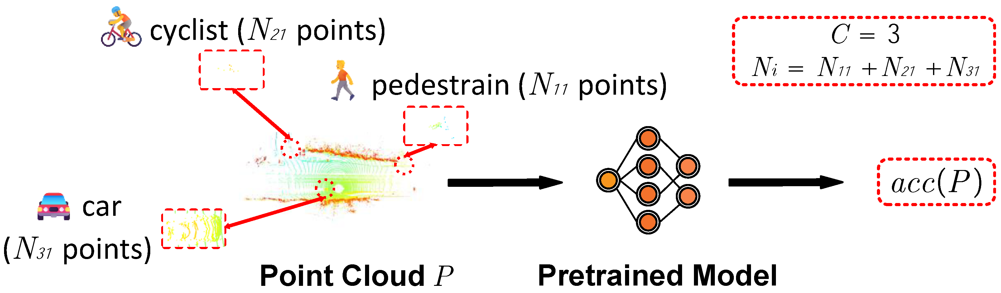
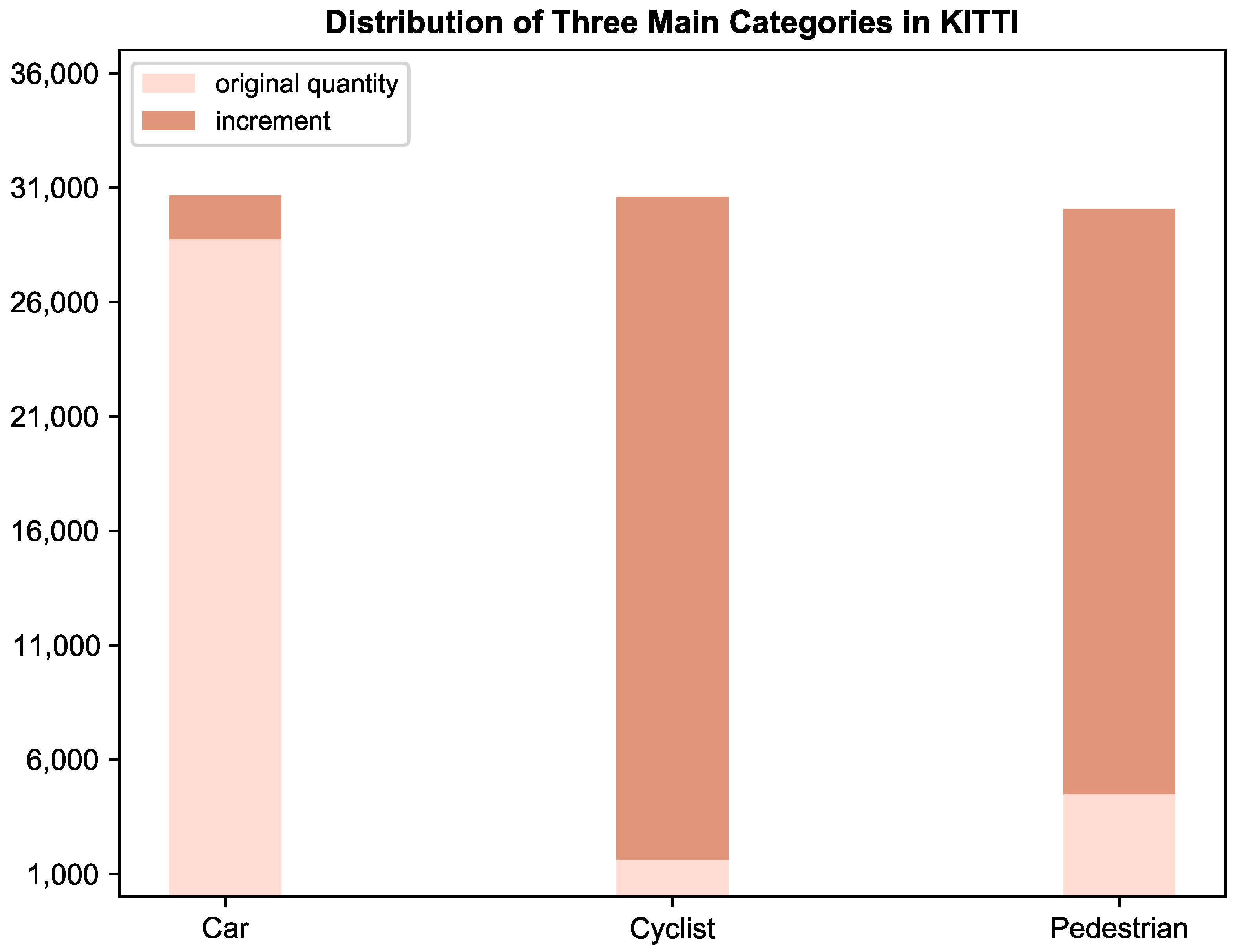
- In order to mitigate the class imbalance issue within the KITTI dataset, this paper further designs an adversarial dataset based on KITTI, which is referred to as Adv-KITTI, by implementing a single-frame ground truth augmentation technique named SFGTS, which creates a complementary dataset of copious object meshes.
- A novel variant of focal loss is formulated, which allows the developed detector to distinguish between challenging and simple objects, substantially intensifying the attentiveness to strenuous ones through the adaptive modulation of hyperparameters.
2. Related Works
2.1. LiDAR-Based 3D Object Detection
2.2. Adversarial Attack on 2D Image Vision
2.3. LiDAR Detectors with Adversarial Attack
3. Background
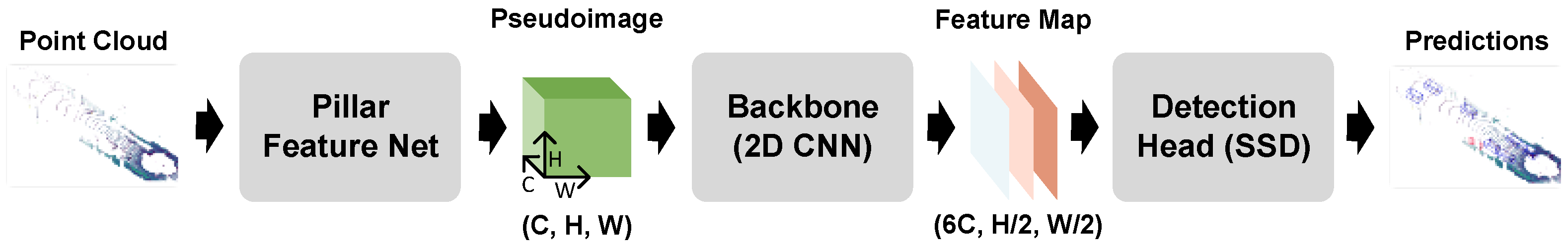
3.1. Preliminaries : PointPillars
3.2. Preliminaries : FGSM
3.3. Motivation
4. Methodology
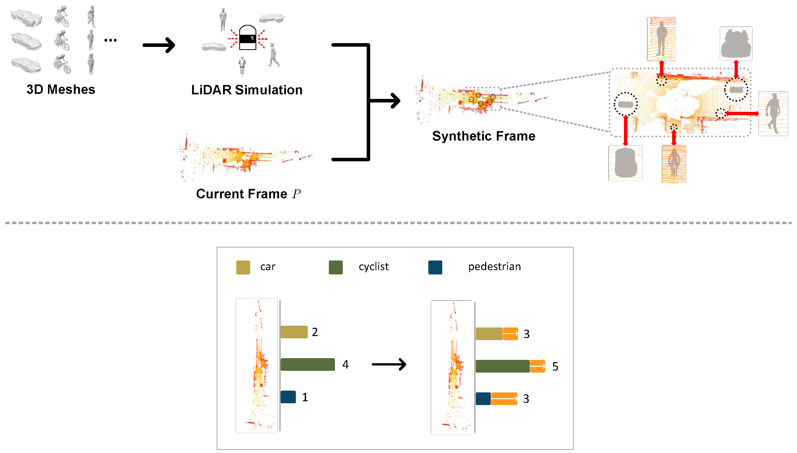
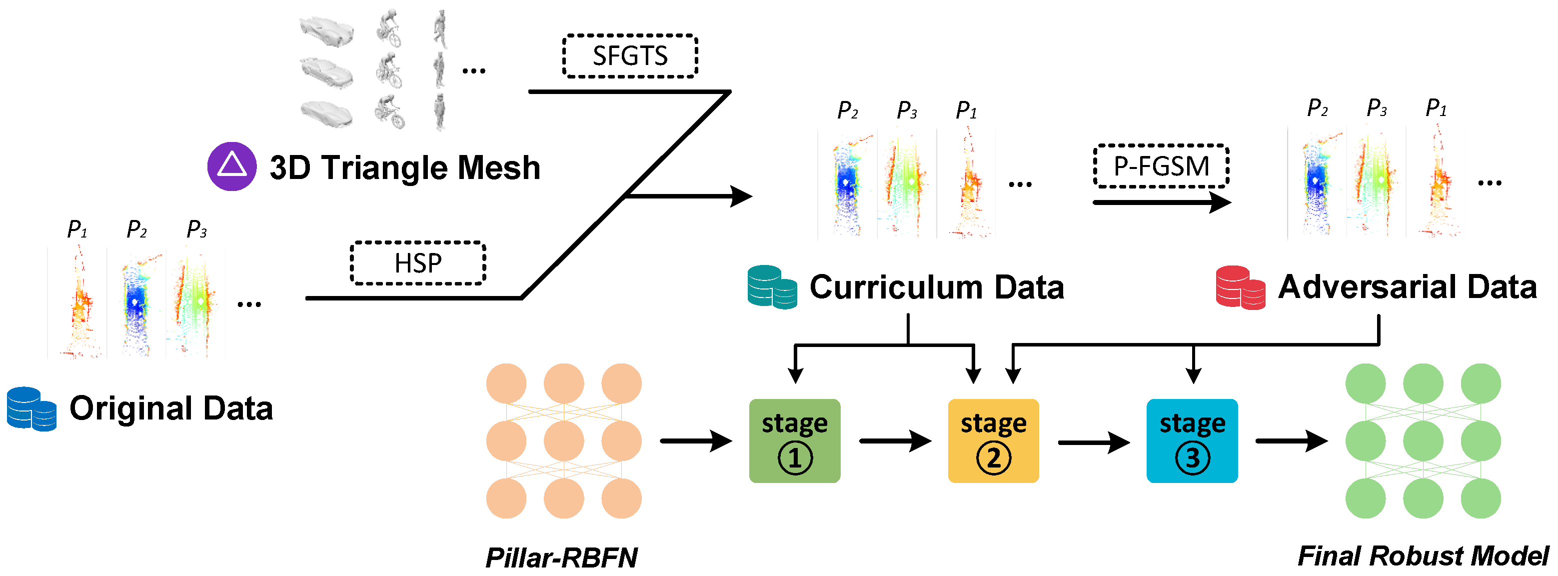
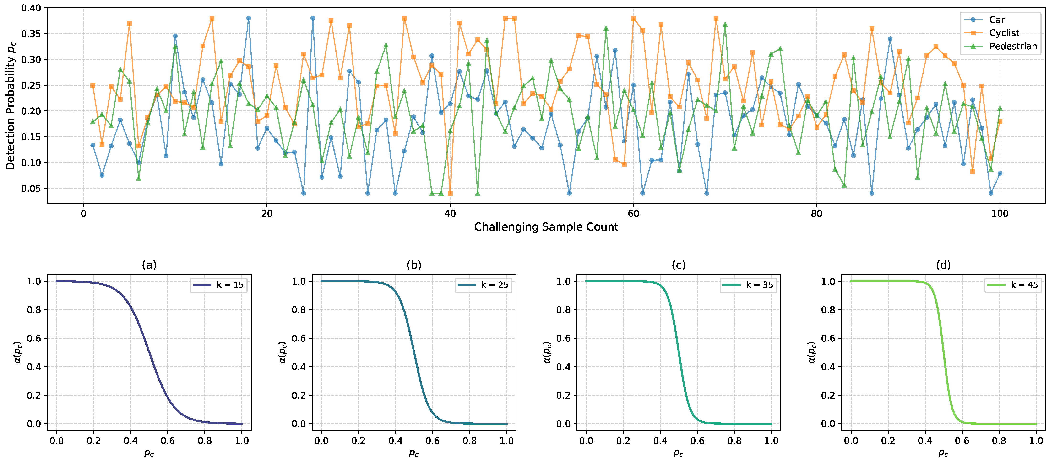
4.1. Hierarchical Sample Partition
4.2. Generation of Adversarial Examples
| Algorithm 1 Single-frame ground truth sample |
Initialization: minimum quantity ∈ {, , }, maximum quantity ∈ {, , }; Inputs: Point Cloud P, Mesh Dataset ;
|
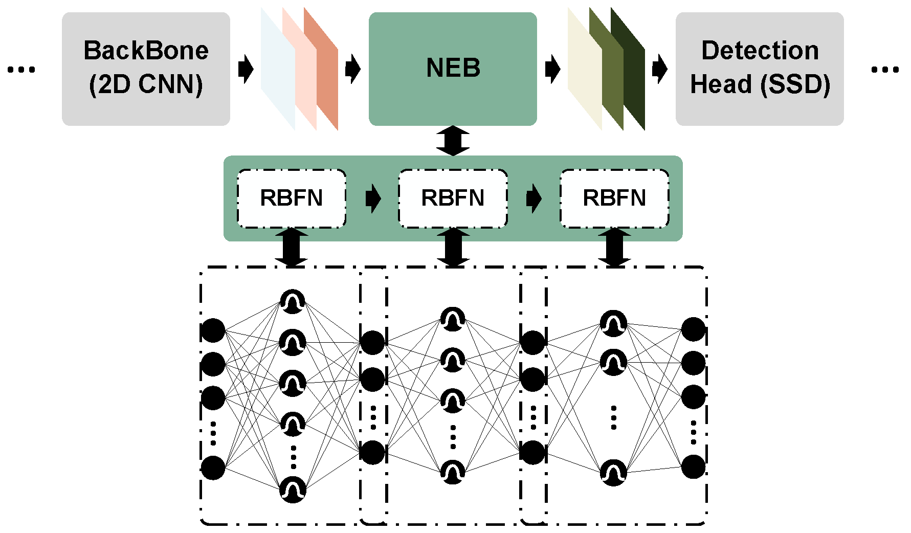
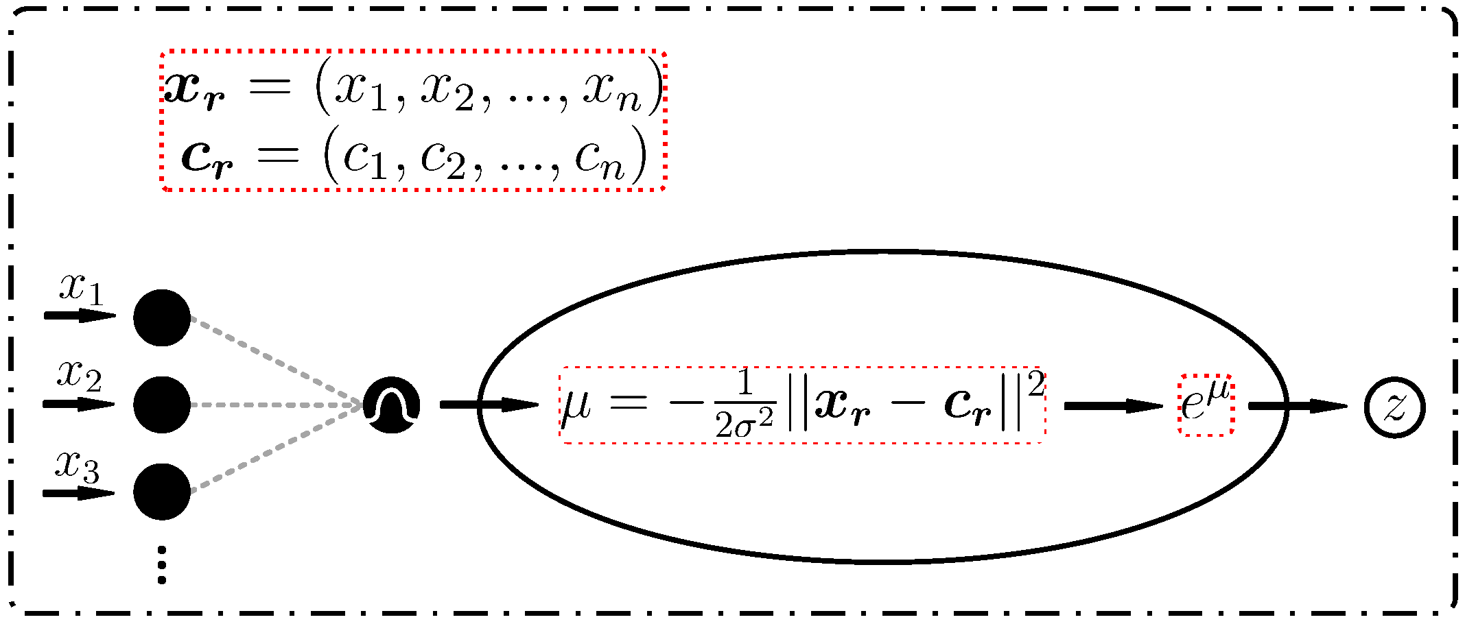
4.3. Nonlinear Enhancement Block
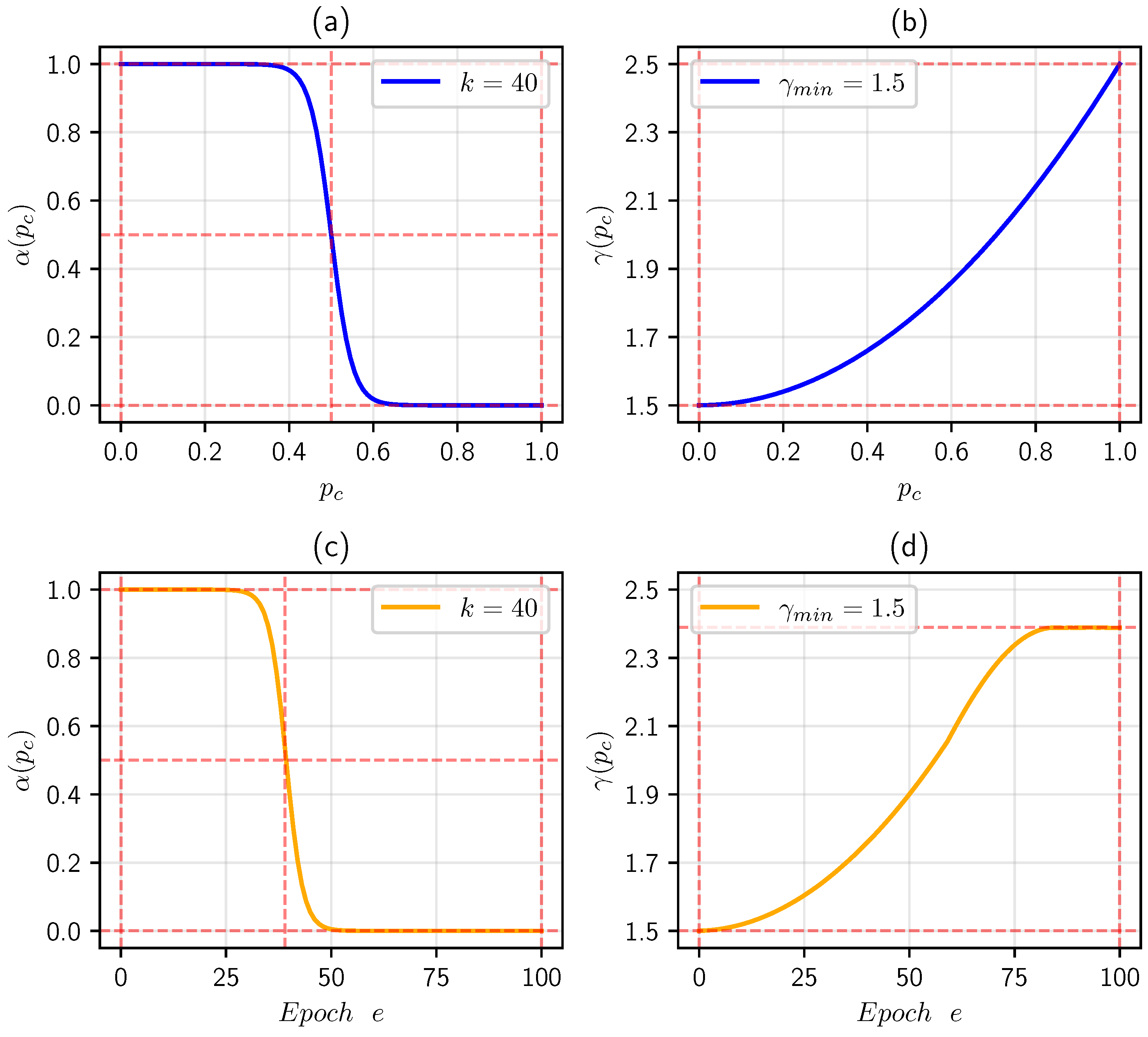
4.4. Robustness Training with Curriculum
- Stage 1: Initial training of PointPillars.
- Stage 2: Adversarial sample generation and joint training.
- Stage 3: Final training on NEB modules.
| Algorithm 2 Robust adversarial training. |
Initialization: exponential factor , sensitivity factor k; Inputs: training split , validation split , epoch e;
|
4.5. Adaptive Class-Balanced Loss
5. Experiment
5.1. Dataset and Preprocessing
5.2. Engaged Models
5.3. Experimental Settings
5.3.1. Basic Settings
5.3.2. Settings on Hyperparameters k and
5.4. Implementation Details
5.4.1. Hierarchical Sample Partition
5.4.2. PointPillars with RBFN
5.4.3. Adversarial Training
5.5. Experimental Results
5.5.1. Curriculum Partitioning Analysis
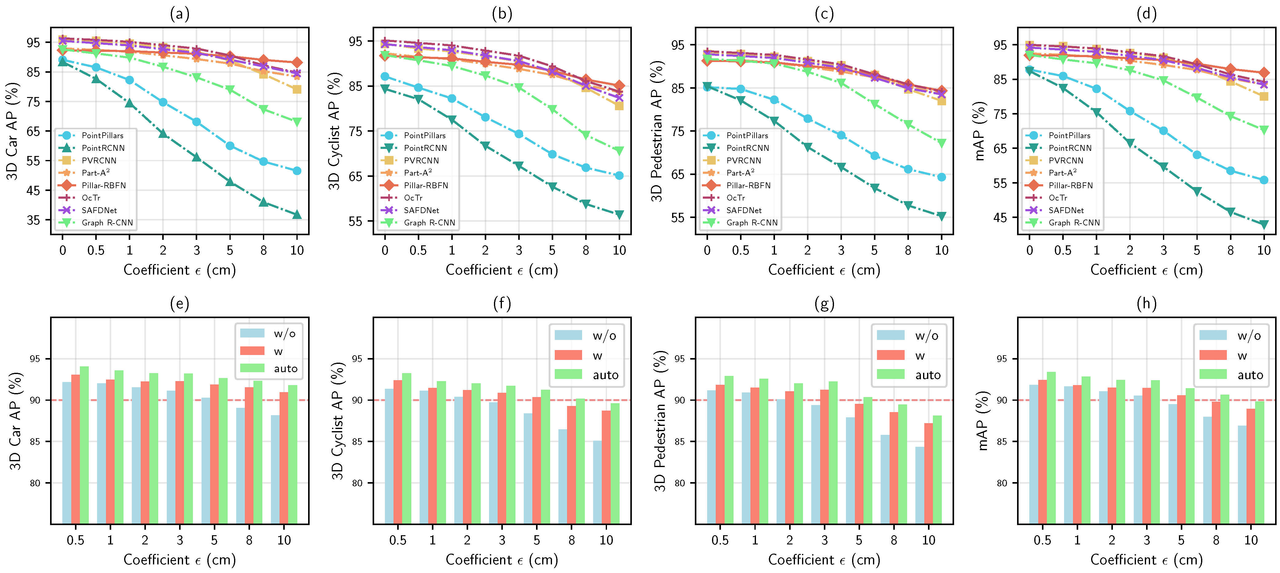
5.5.2. Quantitative Adversarial Robustness Evaluation
- Analysis on different feature representations.
- Analysis on three state-of-the-art modules.
- Analysis on different setting manners.
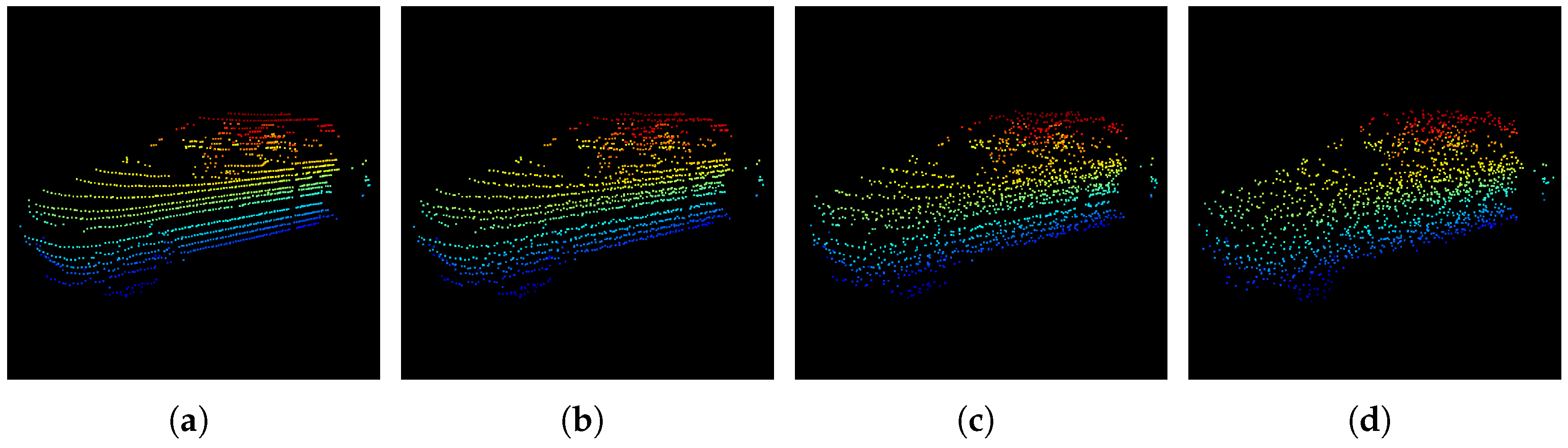
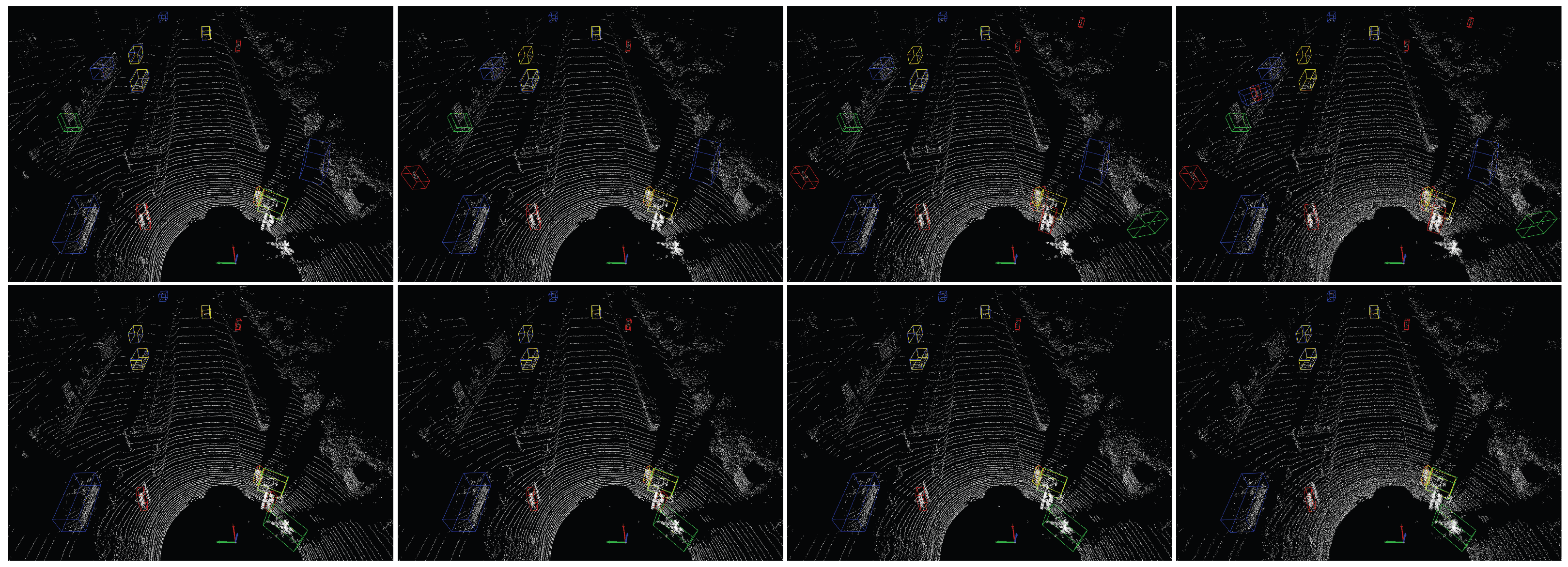
5.5.3. Qualitative Adversarial Robustness Evaluation
5.6. Other Relative Experiments
5.6.1. Adversarial Robustness with Different Pillar Sizes
5.6.2. Ablative Study on Adversarial Robustness Enhancement
6. Discussion
6.1. Potential Practical Applications and Challenges
6.2. Limitations and Future Research Directions
7. Conclusions
Author Contributions
Funding
Institutional Review Board Statement
Informed Consent Statement
Data Availability Statement
Conflicts of Interest
References
- Zamanakos, G.; Tsochatzidis, L.; Amanatiadis, A.; Pratikakis, I. A comprehensive survey of LIDAR-based 3D object detection methods with deep learning for autonomous driving. Comput. Graph. 2021, 99, 153–181. [Google Scholar] [CrossRef]
- Brinatti Vazquez, G.D.; Lacapmesure, A.M.; Martínez, S.; Martínez, O.E. SUPPOSe 3Dge: A Method for Super-Resolved Detection of Surfaces in Volumetric Fluorescence Microscopy. J. Opt. Photonics Res. 2024. [Google Scholar] [CrossRef]
- Liu, H.; Duan, T. Cross-Modal Collaboration and Robust Feature Classifier for Open-Vocabulary 3D Object Detection. Sensors 2025, 25, 553. [Google Scholar] [CrossRef] [PubMed]
- Hu, K.; Chen, Z.; Kang, H.; Tang, Y. 3D vision technologies for a self-developed structural external crack damage recognition robot. Autom. Constr. 2024, 159, 105262. [Google Scholar] [CrossRef]
- Lang, A.H.; Vora, S.; Caesar, H.; Zhou, L.; Yang, J.; Beijbom, O. PointPillars: Fast Encoders for Object Detection From Point Clouds. In Proceedings of the IEEE/CVF Conference on Computer Vision and Pattern Recognition (CVPR), Long Beach, CA, USA, 16–20 June 2019. [Google Scholar]
- Shi, S.; Wang, X.; Li, H. PointRCNN: 3D Object Proposal Generation and Detection From Point Cloud. In Proceedings of the IEEE/CVF Conference on Computer Vision and Pattern Recognition (CVPR), Long Beach, CA, USA, 16–20 June 2019. [Google Scholar]
- Shi, S.; Guo, C.; Jiang, L.; Wang, Z.; Shi, J.; Wang, X.; Li, H. PV-RCNN: Point-Voxel Feature Set Abstraction for 3D Object Detection. In Proceedings of the IEEE/CVF Conference on Computer Vision and Pattern Recognition (CVPR), Virtual, 14–19 June 2020; pp. 10529–10538. [Google Scholar]
- Cao, Y.; Xiao, C.; Cyr, B.; Zhou, Y.; Park, W.; Rampazzi, S.; Chen, Q.A.; Fu, K.; Mao, Z.M. Adversarial sensor attack on lidar-based perception in autonomous driving. In Proceedings of the 2019 ACM SIGSAC Conference on Computer and Communications Security, London, UK, 11–15 November 2019; pp. 2267–2281. [Google Scholar]
- Goodfellow, I.J.; Shlens, J.; Szegedy, C. Explaining and harnessing adversarial examples. In Proceedings of the International Conference on Learning Representations (ICLR), San Diego, CA, USA, 7–9 May 2015. [Google Scholar]
- Abdelfattah, M.; Yuan, K.; Wang, Z.J.; Ward, R. Adversarial attacks on camera-lidar models for 3D car detection. In Proceedings of the 2021 IEEE/RSJ International Conference on Intelligent Robots and Systems (IROS), Prague, Czech Republic, 27 September–1 October 2021; pp. 2189–2194. [Google Scholar]
- Geiger, A.; Lenz, P.; Urtasun, R. Are we ready for autonomous driving? The KITTI vision benchmark suite. In Proceedings of the IEEE/CVF Conference on Computer Vision and Pattern Recognition (CVPR), Providence, RI, USA, 16–21 June 2012; pp. 3354–3361. [Google Scholar]
- Zhang, Y.; Ding, M.; Yang, H.; Niu, Y.; Ge, M.; Ohtani, K.; Zhang, C.; Takeda, K. LiDAR Point Cloud Augmentation for Adverse Conditions Using Conditional Generative Model. Remote Sens. 2024, 16, 2247. [Google Scholar] [CrossRef]
- Fan, X.; Xiao, D.; Li, Q.; Gong, R. Snow-CLOCs: Camera-LiDAR Object Candidate Fusion for 3D Object Detection in Snowy Conditions. Sensors 2024, 24, 4158. [Google Scholar] [CrossRef] [PubMed]
- Shafahi, A.; Najibi, M.; Ghiasi, M.A.; Xu, Z.; Dickerson, J.; Studer, C.; Davis, L.S.; Taylor, G.; Goldstein, T. Adversarial training for free! In Proceedings of the Advances in Neural Information Processing Systems, Vancouver, BC, Canada, 8–14 December 2019; Volume 32. [Google Scholar]
- Bengio, Y.; Louradour, J.; Collobert, R.; Weston, J. Curriculum learning. In Proceedings of the 26th Annual International Conference on Machine Learning, Montreal, QC, Canada, 14–18 June 2009; pp. 41–48. [Google Scholar]
- Zhu, Z.; Meng, Q.; Wang, X.; Wang, K.; Yan, L.; Yang, J. Curricular Object Manipulation in LiDAR-Based Object Detection. In Proceedings of the IEEE/CVF Conference on Computer Vision and Pattern Recognition (CVPR), Vancouver, BC, Canada, 17–24 June 2023; pp. 1125–1135. [Google Scholar]
- Fei, B.; Luo, T.; Yang, W.; Liu, L.; Zhang, R.; He, Y. Curriculumformer: Taming Curriculum Pre-Training for Enhanced 3-D Point Cloud Understanding. IEEE Trans. Neural Netw. Learn. Syst. 2024, 1–15. [Google Scholar] [CrossRef] [PubMed]
- Madry, A.; Makelov, A.; Schmidt, L.; Tsipras, D.; Vladu, A. Towards deep learning models resistant to adversarial attacks. stat 2017, 1050. [Google Scholar]
- Yang, Z.; Sun, Y.; Liu, S.; Jia, J. 3DSSD: Point-Based 3D Single Stage Object Detector. In Proceedings of the IEEE/CVF Conference on Computer Vision and Pattern Recognition (CVPR), Seattle, WA, USA, 13–19 June 2020. [Google Scholar]
- Pan, X.; Xia, Z.; Song, S.; Li, L.E.; Huang, G. 3D Object Detection With Pointformer. In Proceedings of the IEEE/CVF Conference on Computer Vision and Pattern Recognition (CVPR), Nashville, TN, USA, 20–25 June 2021; pp. 7463–7472. [Google Scholar]
- Qi, C.R.; Su, H.; Mo, K.; Guibas, L.J. PointNet: Deep Learning on Point Sets for 3D Classification and Segmentation. In Proceedings of the IEEE/CVF Conference on Computer Vision and Pattern Recognition (CVPR), Honolulu, HI, USA, 21–26 July 2017. [Google Scholar]
- Qi, C.R.; Yi, L.; Su, H.; Guibas, L.J. PointNet++: Deep Hierarchical Feature Learning on Point Sets in a Metric Space. In Proceedings of the Advances in Neural Information Processing Systems, Long Beach, CA, USA, 4–9 December 2017; Volume 30. [Google Scholar]
- Zhou, Y.; Tuzel, O. VoxelNet: End-to-End Learning for Point Cloud Based 3D Object Detection. In Proceedings of the IEEE/CVF Conference on Computer Vision and Pattern Recognition (CVPR), Salt Lake City, UT, USA, 18–23 June 2018. [Google Scholar]
- Yan, Y.; Mao, Y.; Li, B. SECOND: Sparsely Embedded Convolutional Detection. Sensors 2018, 18, 3337. [Google Scholar] [CrossRef] [PubMed]
- Mao, J.; Xue, Y.; Niu, M.; Bai, H.; Feng, J.; Liang, X.; Xu, H.; Xu, C. Voxel Transformer for 3D Object Detection. In Proceedings of the IEEE/CVF International Conference on Computer Vision (ICCV), Montreal, QC, Canada, 11–17 October 2021; pp. 3164–3173. [Google Scholar]
- Tang, H.; Liu, Z.; Zhao, S.; Lin, Y.; Lin, J.; Wang, H.; Han, S. Searching Efficient 3D Architectures with Sparse Point-Voxel Convolution. In Proceedings of the European Conference on Computer Vision (ECCV), Glasgow, UK, 23–28 August 2020; pp. 685–702. [Google Scholar]
- Shi, S.; Jiang, L.; Deng, J.; Wang, Z.; Guo, C.; Shi, J.; Wang, X.; Li, H. PV-RCNN++: Point-voxel feature set abstraction with local vector representation for 3D object detection. Int. J. Comput. Vis. 2023, 131, 531–551. [Google Scholar] [CrossRef]
- Li, Z.; Wang, F.; Wang, N. LiDAR R-CNN: An Efficient and Universal 3D Object Detector. In Proceedings of the IEEE/CVF Conference on Computer Vision and Pattern Recognition (CVPR), Nashville, TN, USA, 20–25 June 2021; pp. 7546–7555. [Google Scholar]
- Hu, J.S.K.; Kuai, T.; Waslander, S.L. Point Density-Aware Voxels for LiDAR 3D Object Detection. In Proceedings of the IEEE/CVF Conference on Computer Vision and Pattern Recognition (CVPR), New Orleans, LA, USA, 18–24 June 2022; pp. 8469–8478. [Google Scholar]
- Liu, Z.; Tang, H.; Lin, Y.; Han, S. Point-Voxel CNN for Efficient 3D Deep Learning. In Proceedings of the Advances in Neural Information Processing Systems, Vancouver, BC, Canada, 8–14 December 2019; Volume 32. [Google Scholar]
- Miao, Z.; Chen, J.; Pan, H.; Zhang, R.; Liu, K.; Hao, P.; Zhu, J.; Wang, Y.; Zhan, X. PVGNet: A Bottom-Up One-Stage 3D Object Detector With Integrated Multi-Level Features. In Proceedings of the IEEE/CVF Conference on Computer Vision and Pattern Recognition (CVPR), Nashville, TN, USA, 20–25 June 2021; pp. 3279–3288. [Google Scholar]
- Szegedy, C. Intriguing properties of neural networks. In Proceedings of the International Conference on Learning Representations (ICLR), Scottsdale, AZ, USA, 2–4 May 2013. [Google Scholar]
- Li, Y.; Xie, B.; Guo, S.; Yang, Y.; Xiao, B. A survey of robustness and safety of 2d and 3d deep learning models against adversarial attacks. ACM Comput. Surv. 2024, 56, 1–37. [Google Scholar] [CrossRef]
- Miyato, T.; Dai, A.M.; Goodfellow, I. Adversarial Training Methods for Semi-Supervised Text Classification. In Proceedings of the International Conference on Learning Representations (ICLR), Toulon, France, 24–26 April 2017. [Google Scholar]
- Moosavi-Dezfooli, S.M.; Fawzi, A.; Frossard, P. Deepfool: A simple and accurate method to fool deep neural networks. In Proceedings of the IEEE Conference on Computer Vision and Pattern Recognition, Las Vegas, NV, USA, 27–30 June 2016; pp. 2574–2582. [Google Scholar]
- Papernot, N.; McDaniel, P.; Jha, S.; Fredrikson, M.; Celik, Z.B.; Swami, A. The limitations of deep learning in adversarial settings. In Proceedings of the IEEE European Symposium on Security and Privacy, Saarbruecken, Germany, 21–24 March 2016; pp. 372–387. [Google Scholar]
- Carlini, N.; Wagner, D. Towards Evaluating the Robustness of Neural Networks. In Proceedings of the 2017 IEEE Symposium on Security and Privacy (SP), San Jose, CA, USA, 22–26 May 2017; pp. 39–57. [Google Scholar]
- Papernot, N.; McDaniel, P.; Wu, X.; Jha, S.; Swami, A. Distillation as a Defense to Adversarial Perturbations Against Deep Neural Networks. In Proceedings of the 2016 IEEE Symposium on Security and Privacy (SP), San Jose, CA, USA, 22–26 May 2016; pp. 582–597. [Google Scholar]
- Chen, P.Y.; Zhang, H.; Sharma, Y.; Yi, J.; Hsieh, C.J. Zoo: Zeroth order optimization based black-box attacks to deep neural networks without training substitute models. In Proceedings of the 10th ACM Workshop on Artificial Intelligence and Security, Dallas, TX, USA, 3 November 2017; pp. 15–26. [Google Scholar]
- Papernot, N.; McDaniel, P.D.; Goodfellow, I.J.; Jha, S.; Celik, Z.B.; Swami, A. Practical Black-Box Attacks against Deep Learning Systems using Adversarial Examples. In Proceedings of the ACM on Asia Conference on Computer and Communications Security, Xi’an, China, 30 May–3 June 2016. [Google Scholar]
- Brendel, W.; Rauber, J.; Bethge, M. Decision-based adversarial attacks: Reliable attacks against black-box machine learning models. In Proceedings of the International Conference on Learning Representations (ICLR), Toulon, France, 24–26 April 2017. [Google Scholar]
- Chen, S.; He, Z.; Sun, C.; Huang, X. Universal Adversarial Attack on Attention and the Resulting Dataset DAmageNet. IEEE Trans. Pattern Anal. Mach. Intell. 2020, 44, 2188–2197. [Google Scholar] [CrossRef] [PubMed]
- Chen, Z.; Li, B.; Wu, S.; Jiang, K.; Ding, S.; Zhang, W. Content-based Unrestricted Adversarial Attack. In Proceedings of the Advances in Neural Information Processing Systems, New Orleans, LA, USA, 10–16 December 2023; pp. 51719–51733. [Google Scholar]
- Lehner, A.; Gasperini, S.; Marcos-Ramiro, A.; Schmidt, M.; Mahani, M.A.N.; Navab, N.; Busam, B.; Tombari, F. 3d-vfield: Adversarial augmentation of point clouds for domain generalization in 3d object detection. In Proceedings of the IEEE/CVF Conference on Computer Vision and Pattern Recognition (CVPR), New Orleans, LA, USA, 18–24 June 2022; pp. 17295–17304. [Google Scholar]
- Tu, J.; Ren, M.; Manivasagam, S.; Liang, M.; Yang, B.; Du, R.; Cheng, F.; Urtasun, R. Physically realizable adversarial examples for lidar object detection. In Proceedings of the IEEE/CVF Conference on Computer Vision and Pattern Recognition (CVPR), Seattle, WA, USA, 13–19 June 2020; pp. 13716–13725. [Google Scholar]
- Tu, J.; Li, H.; Yan, X.; Ren, M.; Chen, Y.; Liang, M.; Bitar, E.; Yumer, E.; Urtasun, R. Exploring adversarial robustness of multi-sensor perception systems in self driving. In Proceedings of the 5th Annual Conference on Robot Learning, London, UK, 8–11 November 2021. [Google Scholar]
- Sun, J.; Cao, Y.; Chen, Q.A.; Mao, Z.M. Towards robust {LiDAR-based} perception in autonomous driving: General black-box adversarial sensor attack and countermeasures. In Proceedings of the 29th USENIX Security Symposium (USENIX Security 20), Berkeley, CA, USA, 12–14 August 2020; pp. 877–894. [Google Scholar]
- Cai, M.; Wang, X.; Sohel, F.; Lei, H. Unsupervised Anomaly Detection for Improving Adversarial Robustness of 3D Object Detection Models. Electronics 2025, 14, 236. [Google Scholar] [CrossRef]
- Zhu, S.; Zhao, Y.; Chen, K.; Wang, B.; Ma, H.; Wei, C. AE-Morpher: Improve Physical Robustness of Adversarial Objects against LiDAR-based Detectors via Object Reconstruction. In Proceedings of the 33rd USENIX Security Symposium (USENIX Security 24), Philadelphia, PA, USA, 14–16 August 2024; pp. 7339–7356. [Google Scholar]
- Girshick, R. Fast R-CNN. In Proceedings of the IEEE/CVF International Conference on Computer Vision (ICCV), Santiago, Chile, 7–13 December 2015. [Google Scholar]
- Lin, T.Y.; Goyal, P.; Girshick, R.; He, K.; Dollar, P. Focal Loss for Dense Object Detection. In Proceedings of the IEEE/CVF International Conference on Computer Vision (ICCV), Venice, Italy, 22–29 October 2017. [Google Scholar]
- Caesar, H.; Bankiti, V.; Lang, A.H.; Vora, S.; Liong, V.E.; Xu, Q.; Krishnan, A.; Pan, Y.; Baldan, G.; Beijbom, O. nuscenes: A multimodal dataset for autonomous driving. In Proceedings of the IEEE/CVF Conference on Computer Vision and Pattern Recognition (CVPR), Seattle, WA, USA, 13–19 June 2020; pp. 11621–11631. [Google Scholar]
- Zhou, H.; Zhu, X.; Song, X.; Ma, Y.; Wang, Z.; Li, H.; Lin, D. Cylinder3d: An effective 3d framework for driving-scene lidar semantic segmentation. In Proceedings of the IEEE/CVF Conference on Computer Vision and Pattern Recognition (CVPR), Seattle, WA, USA, 13–19 June 2020. [Google Scholar]
- Park, J.; Sandberg, I.W. Universal Approximation Using Radial-Basis-Function Networks. Neural Comput. 1991, 3, 246–257. [Google Scholar] [CrossRef] [PubMed]
- Shi, S.; Wang, Z.; Shi, J.; Wang, X.; Li, H. From Points to Parts: 3D Object Detection From Point Cloud With Part-Aware and Part-Aggregation Network. IEEE Trans. Pattern Anal. Mach. Intell. 2021, 43, 2647–2664. [Google Scholar] [CrossRef] [PubMed]
- Wei, S.; Yang, Y.; Liu, D.; Deng, K.; Wang, C. Transformer-Based Spatiotemporal Graph Diffusion Convolution Network for Traffic Flow Forecasting. Electronics 2024, 13, 3151. [Google Scholar] [CrossRef]
- Zhou, C.; Zhang, Y.; Chen, J.; Huang, D. OcTr: Octree-Based Transformer for 3D Object Detection. In Proceedings of the IEEE/CVF Conference on Computer Vision and Pattern Recognition (CVPR), Vancouver, BC, Canada, 17–24 June 2023; pp. 5166–5175. [Google Scholar]
- Zhang, G.; Chen, J.; Gao, G.; Li, J.; Liu, S.; Hu, X. SAFDNet: A Simple and Effective Network for Fully Sparse 3D Object Detection. In Proceedings of the IEEE/CVF Conference on Computer Vision and Pattern Recognition (CVPR), Seattle, WA, USA, 16–22 June 2024; pp. 14477–14486. [Google Scholar]
- Yang, H.; Liu, Z.; Wu, X.; Wang, W.; Qian, W.; He, X.; Cai, D. Graph R-CNN: Towards Accurate 3D Object Detection with Semantic-Decorated Local Graph. In Proceedings of the European Conference on Computer Vision (ECCV), Tel Aviv, Israel, 23–27 October 2022; pp. 662–679. [Google Scholar]
- Behley, J.; Garbade, M.; Milioto, A.; Quenzel, J.; Behnke, S.; Stachniss, C.; Gall, J. Semantickitti: A dataset for semantic scene understanding of lidar sequences. In Proceedings of the IEEE/CVF International Conference on Computer Vision (ICCV), Seoul, Republic of Korea, 27 October–2 November 2019; pp. 9297–9307. [Google Scholar]


| Method | Modality | Representation | Feature Extraction | Memory Footprint | |||||||
|---|---|---|---|---|---|---|---|---|---|---|---|
| Point | Voxel | Pillar | 2D cnn | 3d cnn | Transformer | Set Abstraction | L | M | H | ||
| PointRCNN [6] | PB | ✔ | - | - | - | - | - | ✔ | - | - | ✔ |
| 3DSSD [19] | PB | ✔ | - | - | - | - | - | ✔ | - | - | ✔ |
| Pointformer [20] | PB | ✔ | - | - | - | - | ✔ | - | - | ✔ | - |
| PointPillars [5] | GB | - | - | ✔ | ✔ | - | - | - | ✔ | - | - |
| SECOND [24] | GB | - | ✔ | - | ✔ | ✔ | - | - | - | ✔ | - |
| VoxelNet [23] | GB | - | ✔ | - | - | - | - | ✔ | - | - | ✔ |
| VoTr-SSD [25] | GB | - | ✔ | - | ✔ | - | ✔ | - | - | ✔ | - |
| k | mAP (%) | Recall (%) | Epoch | |
|---|---|---|---|---|
| 35 | 1.0 | 87.31 | 72.50 | 124 |
| 35 | 1.5 | 88.64 | 73.82 | 116 |
| 35 | 2.0 | 87.90 | 73.13 | 118 |
| 35 | 2.5 | 89.47 | 74.56 | 115 |
| 40 | 1.0 | 90.24 | 76.71 | 104 |
| 40 | 1.5 | 91.97 | 78.90 | 101 |
| 40 | 2.0 | 90.68 | 77.54 | 106 |
| 45 | 1.0 | 89.52 | 75.28 | 110 |
| 45 | 1.5 | 90.10 | 76.10 | 112 |
| 45 | 2.0 | 89.34 | 74.83 | 108 |
| 50 | 1.0 | 86.75 | 70.92 | 116 |
| Method | Modality | mAP (%) | 3D Car AP (%) | 3D Cyclist AP (%) | 3D Pedestrian AP (%) | ||||
|---|---|---|---|---|---|---|---|---|---|
| RS | CA | RS | CA | RS | CA | RS | CA | ||
| PointPillars [5] | LiDAR | 69.11 | 69.79 | 78.59 | 79.17 | 69.82 | 70.68 | 58.94 | 59.51 |
| PointRCNN [6] | LiDAR | 69.84 | 70.61 | 79.18 | 80.24 | 70.12 | 70.86 | 60.22 | 60.73 |
| PVRCNN [7] | LiDAR | 74.59 | 75.19 | 82.70 | 83.41 | 74.37 | 74.95 | 66.71 | 67.20 |
| Part-A2 [55] | LiDAR | 73.72 | 74.38 | 80.51 | 81.48 | 76.90 | 77.43 | 63.76 | 64.24 |
| Graph R-CNN [59] | LiDAR | 74.64 | 75.33 | 82.57 | 83.32 | 74.78 | 75.47 | 66.58 | 67.21 |
| OcTr [57] | LiDAR | 75.82 | 76.48 | 83.72 | 84.45 | 75.91 | 76.58 | 67.83 | 68.42 |
| SAFDNet [58] | LiDAR | 75.34 | 76.03 | 83.28 | 84.02 | 75.45 | 76.12 | 67.30 | 67.96 |
| Pillar-RBFN (ours) | LiDAR | 71.51 | 72.08 | 80.26 | 81.02 | 72.45 | 72.86 | 61.82 | 62.37 |
| Method | Modality | mAP (%) | 3D Car AP (%) | 3D Cyclist AP (%) | 3D Pedestrian AP (%) | ||||
|---|---|---|---|---|---|---|---|---|---|
| GTS | HSP | GTS | HSP | GTS | HSP | GTS | HSP | ||
| PointPillars [5] | LiDAR | 85.73 | 87.13 | 87.23 | 89.08 | 86.35 | 87.14 | 83.60 | 85.17 |
| PointRCNN [6] | LiDAR | 85.06 | 86.03 | 87.42 | 88.36 | 82.84 | 84.36 | 84.91 | 85.38 |
| PVRCNN [7] | LiDAR | 92.82 | 94.37 | 95.17 | 95.86 | 92.56 | 94.38 | 90.73 | 92.87 |
| Part-A2 [55] | LiDAR | 90.56 | 92.26 | 91.80 | 92.94 | 90.12 | 92.26 | 89.76 | 91.58 |
| Graph R-CNN [59] | LiDAR | 88.59 | 89.96 | 89.45 | 90.83 | 88.32 | 89.67 | 88.01 | 89.38 |
| OcTr [57] | LiDAR | 93.20 | 94.62 | 95.42 | 96.18 | 93.25 | 94.72 | 90.92 | 92.95 |
| SAFDNet [58] | LiDAR | 91.19 | 92.89 | 92.87 | 93.95 | 91.08 | 92.67 | 89.63 | 91.42 |
| Pillar-RBFN (ours) | LiDAR | 89.57 | 91.73 | 90.31 | 92.17 | 89.66 | 91.74 | 88.58 | 91.28 |
| PointPillars [5] (%) | Ours (%) | |||||
|---|---|---|---|---|---|---|
| 0.18 m | 64.73 | 36.29 | 8.20 | 73.18 | 72.93 | 70.46 |
| 0.20 m | 61.32 | 30.42 | 11.34 | 73.60 | 72.11 | 69.27 |
| 0.22 m | 59.26 | 34.15 | 5.71 | 72.64 | 71.14 | 68.80 |
| 0.24 m | 62.12 | 27.94 | 14.90 | 72.05 | 70.83 | 68.54 |
| 0.26 m | 58.40 | 22.03 | 10.57 | 72.34 | 71.62 | 66.82 |
| NEB | HSP | CRT | mAP (%) | ||
|---|---|---|---|---|---|
| ✘ | ✘ | ✘ | 62.12 | 27.94 | 14.90 |
| ✔ | ✘ | ✘ | 72.05 | 70.83 | 68.54 |
| ✔ | ✔ | ✘ | 91.65 | 89.49 | 86.90 |
| ✔ | ✘ | ✔ | 73.52 | 71.73 | 68.75 |
| ✔ | ✔ | ✔ | 91.80 | 90.58 | 88.96 |
| CL | AT | mAP (%) | ||
|---|---|---|---|---|
| ✘ | ✘ | 71.22 | 68.94 | 64.96 |
| ✔ | ✘ | 72.69 | 70.30 | 66.35 |
| ✔ | ✔ | 73.47 | 71.79 | 68.72 |
| NEB | CRT | mAP (%) |
|---|---|---|
| ✘ | ✘ | 18.52 |
| ✔ | ✘ | 69.76 |
| ✔ | ✔ | 71.10 |
Disclaimer/Publisher’s Note: The statements, opinions and data contained in all publications are solely those of the individual author(s) and contributor(s) and not of MDPI and/or the editor(s). MDPI and/or the editor(s) disclaim responsibility for any injury to people or property resulting from any ideas, methods, instructions or products referred to in the content. |
© 2025 by the authors. Licensee MDPI, Basel, Switzerland. This article is an open access article distributed under the terms and conditions of the Creative Commons Attribution (CC BY) license (https://creativecommons.org/licenses/by/4.0/).
Share and Cite
Huang, J.; Xie, Y.; Chen, Z.; Su, Y. Curriculum-Guided Adversarial Learning for Enhanced Robustness in 3D Object Detection. Sensors 2025, 25, 1697. https://doi.org/10.3390/s25061697
Huang J, Xie Y, Chen Z, Su Y. Curriculum-Guided Adversarial Learning for Enhanced Robustness in 3D Object Detection. Sensors. 2025; 25(6):1697. https://doi.org/10.3390/s25061697
Chicago/Turabian StyleHuang, Jinzhe, Yiyuan Xie, Zhuang Chen, and Ye Su. 2025. "Curriculum-Guided Adversarial Learning for Enhanced Robustness in 3D Object Detection" Sensors 25, no. 6: 1697. https://doi.org/10.3390/s25061697
APA StyleHuang, J., Xie, Y., Chen, Z., & Su, Y. (2025). Curriculum-Guided Adversarial Learning for Enhanced Robustness in 3D Object Detection. Sensors, 25(6), 1697. https://doi.org/10.3390/s25061697