Abstract
This study establishes a homogeneous half-space and a horizontally layered two-layer background stratigraphy model using cross-borehole electrical resistivity tomography (ERT) based on an incomplete Gauss–Newton (IGN) method to investigate the resistivity inversion characteristics of CO2 storage zones. The effects of storage zone volume (), storage zone resistivity (), background formation resistivity (), and CO2 diffusion on inversion results were systematically analyzed, and the mechanisms underlying the influence of different parameters on inversion imaging were explored. The results indicate that an increase in the significantly affects the inverted resistivity. The can be well inverted within a certain range, but inversion accuracy decreases once the resistivity exceeds a threshold. The is a critical factor influencing inversion results; as the increases, the inverted resistivity values rise markedly, although this effect exhibits an upper limit. The study also uncovers the exponential nature of CO2 diffusion in the storage zone, where diffusion leads to exponential changes in resistivity and the delineation of the diffusion zone is enhanced by comparing pre- and post-injection resistivity differences. These findings offer valuable insights for CO2 storage monitoring, contributing to both safety assessments and the evaluation of storage stability in geological sequestration.
1. Introduction
As global efforts to reduce greenhouse gas emissions intensify, carbon capture and storage (CCS) has emerged as a crucial technology for addressing the growing challenge of atmospheric CO2 levels. The geological storage of CO2 provides a sustainable solution to storing large quantities of COCO2 underground, preventing its release into the atmosphere and thereby reducing the greenhouse effect. Moreover, geological storage is a long-term solution that can sequester CO2 for centuries, helping to stabilize the global climate and meet international carbon reduction targets [1]. However, a significant challenge remains: ensuring the long-term stability and safety of CO2 storage in these reservoirs over extended periods. This challenge necessitates the development and implementation of effective monitoring strategies that can continuously assess the storage zones, ensuring the integrity of the sequestration process and minimizing potential environmental risks [2,3,4].
Continuous monitoring of changes in the subsurface distribution of CO2 is crucial for evaluating the effectiveness and safety of the sequestration process. Reservoir geophysical imaging provides insights into the properties of the formations, with resistivity serving as one of the most critical parameters. The resistivity of geological formations is influenced by the conductivity of rocks and minerals, which varies across the Earth’s crust. These differences in conductivity make resistivity an important indicator for detecting changes in subsurface material structures [5]. Electrical resistivity tomography (ERT) is a widely adopted geophysical technique that offers high sensitivity to variations in the resistivity of pore fluids and the different types of rocks present in the subsurface [6,7,8]. Several advantages of ERT include its ease of implementation, non-invasive nature, cost-effectiveness, high spatial resolution, and relatively high efficiency [9,10,11,12,13]. The injection of high-resistivity CO2 could induce significant changes in the resistivity of the formation. This sensitivity to resistivity contrasts between rocks, pore fluids, and injected CO2 make ERT a powerful tool for tracking CO2 movement and migration within the reservoir. By measuring and analyzing changes in physical parameters such as resistivity before and after injection, it becomes possible to effectively estimate variations in CO2 within the storage zone, which also provides valuable information on the migration pathways and spatial distribution of CO2 in the reservoir over time.
Electrical resistivity tomography (ERT) offers detailed imaging of subsurface resistivity distributions, leveraging its high sensitivity to changes in liquid and gas saturation to monitor geological CO2 storage effectively. Lochbühler et al. [14] introduced a probabilistic inversion method that delivers robust CO2 distribution estimates by providing the full posterior probability density function of the saturation field, enriched by rock physics parameters linking resistivity to saturation. Breen et al. [15] demonstrated ERT’s ability to accurately map the shape, size, and position of CO2 plumes in a brine-saturated porous medium, though it overestimated brine saturation, highlighting data quality challenges over time. Nakatsuka et al. [16] confirmed that CO2 injection into brine-saturated zones increases resistivity, with clay presence reducing conductivity, based on lab and well-logging data from the Nagaoka site. Jia et al. [17] and Al et al. [18] enhanced inter-well ERT systems through optimized electrode arrays, successfully locating CO2-bearing zones, though discrepancies between ERT-imaged and -modeled sequestration zone shapes suggest a need for improved modeling and calibration.
Recent advances in multimodal monitoring underscore the potential of electrical resistivity tomography (ERT) when integrated with advanced sensor systems and complementary geophysical methods. At the Ketzin CO2 pilot site, integrated seismic–ERT monitoring utilized high-stability electrode arrays—designed with corrosion-resistant materials and optimized contact impedance—to achieve a 20% improvement in plume boundary definition accuracy compared to single-method approaches [19]. The CaMI_FRS trials showcased fiber-optic integrated ERT sensors, leveraging distributed sensing capabilities to enable joint inversion with cross-well electromagnetic methods, resulting in a 15% enhancement in CO2 saturation mapping resolution [20]. Further innovations in sensor design for extreme environments include cryogenic-grade electrodes, engineered with low-temperature conductive alloys for permafrost monitoring at −40 °C [21], and refractory sensor packages, featuring thermally resilient coatings to maintain measurement fidelity in 1200 °C molten oxide conditions [22]. These sensor-driven advancements not only improve ERT’s sensitivity and spatial resolution but also expand its applicability as a standalone and hybrid monitoring solution for carbon sequestration, aligning with the evolving demands of subsurface sensing technologies.
At present, significant progress has been made in the application of ERT technology in CO2 storage projects [23,24,25]. For example, in the Ketzin pilot CO2 sequestration project in Germany, both borehole-to-surface and inter-well ERT measurements confirmed that CO2 injection generates significant electrical signals at subsurface electrodes. This finding facilitates the real-time monitoring of the electrode potential, enhancing the capability to track changes in the subsurface environment during CO2 sequestration [24,26]. In addition, the joint inversion of seismic full-waveform inversion (FWI) and inter-well ERT provided three-dimensional models of geophysical parameters and their temporal variations. The real data from the Ketzin pilot project were used to test this joint inversion approach, revealing that CO2 injection resulted in a twofold increase in the resistivity of the sequestration zone [27,28]. Similarly, in the CaMI project in Canada, permanently installed monitoring electrodes successfully detected small amounts of injected CO2. The CO2 saturation derived from inversion showed a strong correlation with the actual amount of CO2 injected at the field research station, highlighting the reliability of the monitoring system for detecting and quantifying CO2 sequestration [29,30,31]. At the Svelvik CO2 pilot site, four monitoring wells were drilled to a depth of 100 m, each equipped with 16 electrodes. The impacts of CO2 injection on formation saturation and pore pressure were effectively monitored, further demonstrating the capability of ERT for the real-time subsurface monitoring of CO2 storage [32].
Despite these advancements, current research still lacks quantitative evaluations of the imaging performance of the resistivity method in CO2 storage zones. To address this gap, our study isolates the intrinsic coupling of CO2 storage parameters (, , and ) with inversion signatures using a fixed-geometry approach. While operational factors like electrode spacing and depth sensitivity have been systematically addressed in prior work [33,34], this analysis decouples geological influences from acquisition configurations to highlight core petrophysical trends. This study uses a resistivity inversion simulation method based on an IGN algorithm to analyze the effects of various factors such as storage zone volume, resistivity, background resistivity, and CO2 diffusion on resistivity inversion results. We investigate the influence of these factors on inversion outcomes and identify the extent of CO2 diffusion regions. The findings from this study are expected to provide valuable insights and practical guidance for the monitoring of CO2 sequestration in future geological storage projects, thereby improving the efficiency and accuracy of CO2 monitoring systems.
2. Methods
The resistivity inversion is a widely used computational technique in geophysical exploration, which enables the estimation of subsurface resistivity distributions. This technique involves measuring potential differences between surface or subsurface electrodes and applying known supply currents to infer the resistivity properties of underground media. The process typically aims to minimize the discrepancy between observed data and theoretical models, leveraging mathematical models and algorithms to reconstruct the subsurface resistivity distribution [35].
The inversion methods can be broadly categorized into two types: linear and nonlinear [36]. The key aspect is the establishment of a mathematical relationship between the observed data and the geological model parameters. The linear inversion method, using parameter substitution and Taylor series expansion, transforms nonlinear inverse problems into linear ones. These methods are particularly advantageous due to their excellent convergence behaviors, especially in multidimensional problems, and have thus become one of the most robust, widely applied, and effective approaches in geophysical practice. However, linear inversion methods often make simplifying assumptions that may not fully capture the complexities of real-world geological systems. In contrast, nonlinear inversion methods offer distinct advantages, as they are better suited to handle the inherent complexities and nonlinearity of most geophysical problems. These methods avoid the common issue of converging to local minima during iterative inversion, thereby providing more reliable solutions for complex geological scenarios, which is essential for accurately modeling subsurface structures, particularly in cases where the relationships between the observed data and geological properties are highly nonlinear.
In this study, we propose a resistivity inversion method based on the IGN method to investigate the inversion properties of the CO2 geological storage area. The main innovation of this method is its efficiency and stability in dealing with large-scale inversion problems, which significantly reduces the amount of calculations compared with traditional methods. In addition, we systematically analyzed the effects of CO2 storage area volume (), storage area resistivity (), background formation resistivity (), and CO2 diffusion on the inversion results. The influence mechanism of these parameters on inversion imaging is revealed. These findings provide new theoretical support and technical guidance for the monitoring of CO2 geological sequestration.
Therefore, this study adopts a nonlinear inversion approach based on the finite element [37] forward modeling of resistivity imaging. A target function is constructed using the IGN method, with detailed derivations of the data term and model term within the target function. Additionally, a resistivity inversion workflow is established, providing a robust theoretical foundation for tackling resistivity inversion problems and enhancing the reliability and accuracy of subsurface resistivity estimations.
2.1. Solution of the Objective Function
The IGN method [38] is an improved version of the standard Gauss–Newton algorithm designed to address some of the computational challenges associated with large-scale inverse problems. In the standard Gauss–Newton method, each iteration involves solving a linear system where the Hessian matrix is approximated by the Jacobian matrix. While this approach is effective, it can be computationally expensive and prone to instability, particularly when dealing with large-scale matrices. The IGN method improves upon this by incorporating a relaxation strategy wherein the solution to the linear system is approximated rather than solved exactly during each iteration. This approximation significantly reduces computational costs while maintaining convergence, making the method particularly suitable for large-scale inverse problems where efficiency is a priority.
2.1.1. Construction of the Objective Function
Resistivity inversion is a process aimed at determining the subsurface electrical structure of a target body based on known measured potential data. The core idea behind this process is as follows: through an iterative approach, the electrical parameter configuration of the model is gradually adjusted. Forward modeling algorithms are applied to generate corresponding predictive data, and the simulated response of these predictions is then compared with the observed data. If the predicted response closely matches the observed data, it can be inferred that the geoelectrical model based on the predicted data is a good approximation of the actual subsurface structure.
However, in resistivity inversion, the number of available observation data points is much smaller than the scale of the model parameters. This characteristic results in an underdetermined inversion problem, where multiple solutions may satisfy the observed data, leading to ambiguity in the inversion results. Moreover, the presence of data errors and noise can make the inversion ill posed. To address these challenges, it is necessary to apply additional constraints to the inversion process, which can help to regularize the inversion, transforming it into a well-posed optimization problem. By formulating resistivity inversion as a regularized optimization problem, the inversion process becomes more stable and reliable, enabling a more accurate reconstruction of subsurface resistivity distributions. In this study, the objective function can be expressed as follows:
where m represents the model parameters, refers to the data terms, corresponds to the model terms, and is the regularization parameter.
2.1.2. Data and Model Terms
Based on previous studies and incorporating the finite element discretization method used in the forward solving process, the point-source potential distribution equation can be formulated as follows [39]:
It can be rewritten as the variational form of the following matrix equation:
where represents the potential distribution at the tetrahedral grid nodes, while denotes the conductivity distribution vector within the region. A is defined as the forward operator in the resistivity space. Based on the theory of resistivity forward modeling, it can be observed that the matrix A is a large sparse matrix that is closely related to the grid discretization and the internal conductivity distribution of the model. q is the right-hand side term containing the point-source distribution.
The observation data vector d is a subset of the potential distribution vector at all grid nodes within the study area:
where Q is the mapping matrix from to d. The objective function of least-squares inversion data is obtained using the Hilbert space approximation:
where is the predicted data vector, which is obtained through forward modeling, is the observed data vector, and is the data weighting matrix. is selected as a diagonal matrix, i.e., , where represents the error of the i-th observed data point.
The data term fit is expressed as the root mean square error (RMS) and is given by the following:
where N is the number of measurements, and the objective variance should be 1 (following a chi-square distribution).
In the calculation of the model term, to construct a smoother model structure, the difference between the model parameters and their adjacent parameters is minimized. The specific mathematical expression is as follows:
where is the initial model value, and C is the model weighting matrix.
The Gauss–Newton method is used to transform Equation (1) into the normal equation form:
Let
Thus, Equation (10) can be simplified as
where H is the Hessian matrix and g is the gradient of the objective function. During the inversion process, the Jacobian matrix needs to be computed and stored. However, due to the large amount of data involved in resistivity inversion imaging, the size of the Jacobian matrix J becomes very large. As a result, directly computing and storing the matrix is avoided.
Haber [40] represents the Jacobian matrix J in the following form:
where is the matrix closely related to the grid discretization of the study model and the internal conductivity distribution, since both Q and B are sparse matrices that can be stored in a compressed format [41] to reduce the data size of the Jacobian matrix.
The approximate solution to Equation (11) is obtained under the condition of effectively reducing computation time without affecting the resistivity inversion results.
2.2. ERT Inversion Process
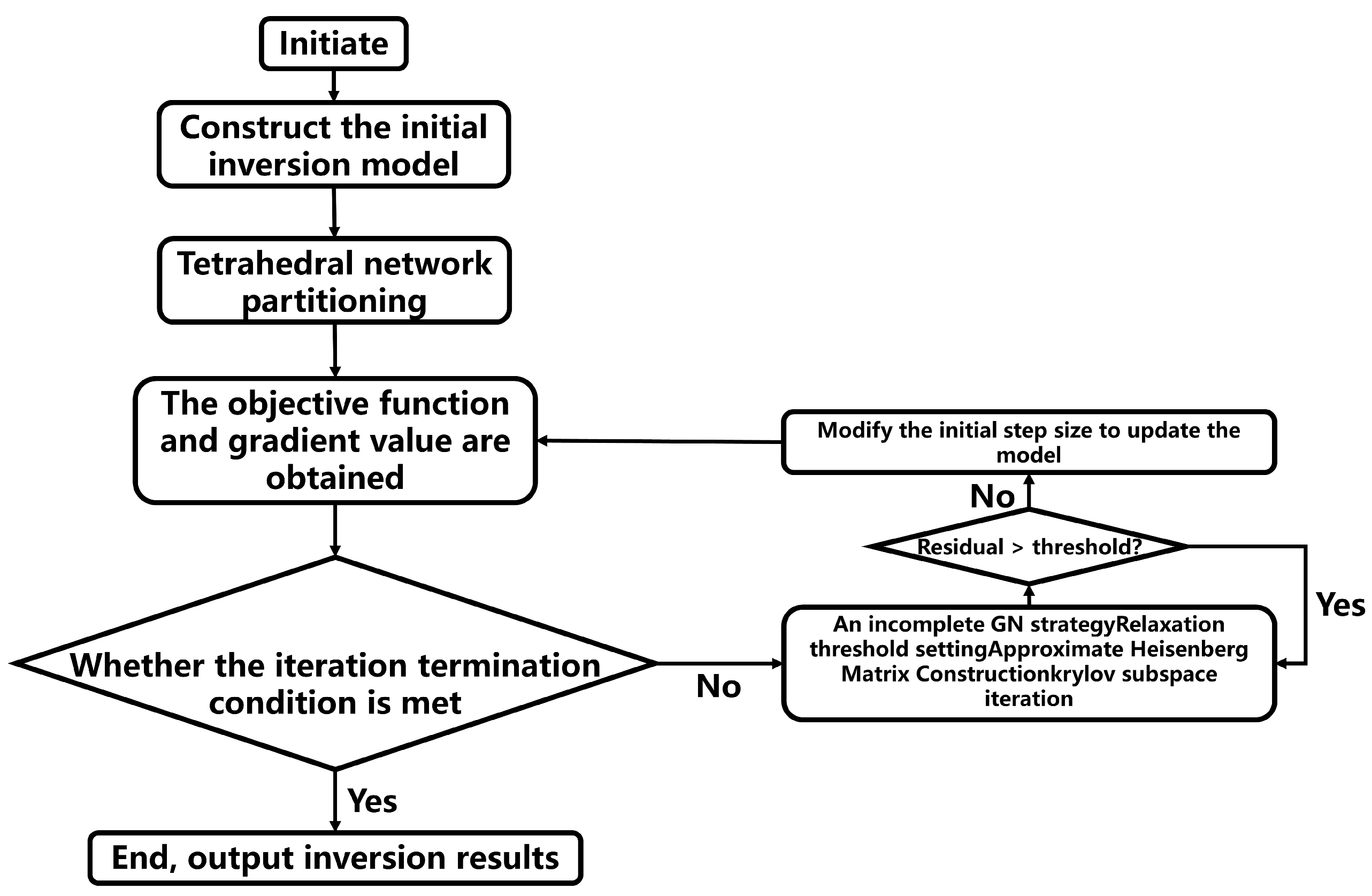
The resistivity inversion process based on finite element forward modeling (FEFM) is an iterative optimization procedure, where the forward and inversion problems are interwoven and solved iteratively (Figure 1). The process begins by defining the initial model, performing a tetrahedral discretization of the study area, and setting the iteration stopping criteria. Once the initial conditions are established, the following steps are carried out:

Figure 1.
Iterative resistivity inversion process based on FEFM.
- The model is discretized using tetrahedral elements, and an initial guess for the conductivity distribution is set. The roughness matrix of the model is computed to understand the initial model’s variations.
- A forward modeling step is performed to simulate the potential distribution based on the current model. This step predicts the data, which are compared to the observed data.
- Objective Function and Gradient Calculation: The objective function, representing the difference between the observed and predicted data, is calculated. The gradient of this function is also computed to determine the direction in which the model needs to be updated.
- The inversion process is iteratively refined. If the value of the objective function falls below a predefined threshold or if the current iteration count exceeds the maximum number of allowed iterations, the process is terminated. Otherwise, the following steps are undertaken.
- The initial step size is adjusted, and the sensitivity matrix is recalculated. The model parameters are updated based on the inversion iteration formula.
- The updated model undergoes another forward response calculation, and the inversion process continues with the next round of iterations. Through this iterative process, the model parameters are refined, progressively improving the fit between the predicted and observed data until the stopping criteria are met.
3. Inversion Model Construction
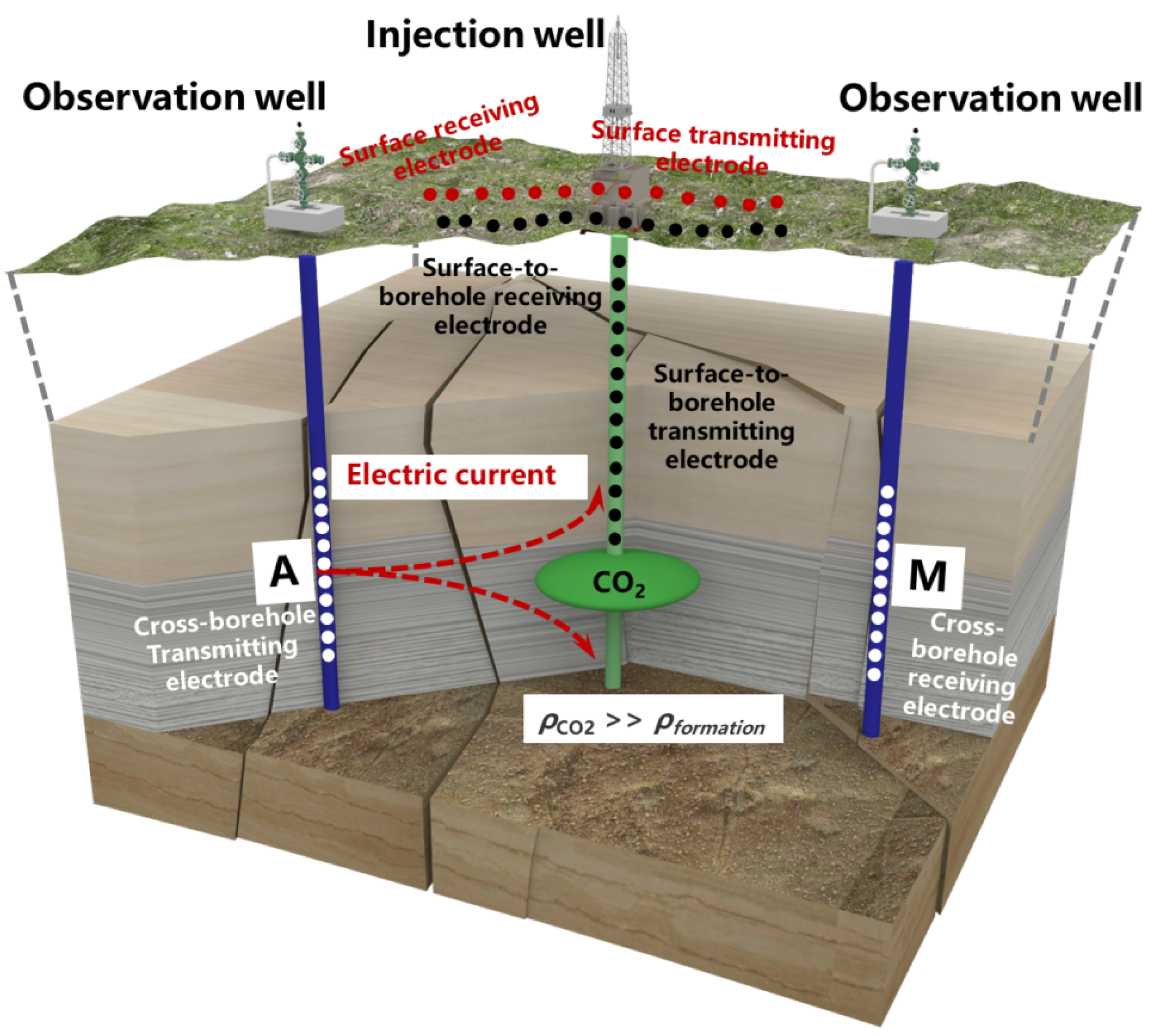
Previous studies have shown that surface ERT imaging is effective for shallow resistivity imaging, where current and potential electrodes are placed on the surface. However, when the measurement depth is too large, the current must travel along a longer path to reach the target area [42,43]. This results in a rapid decay of the electric field strength and a significant reduction in resolution. Existing research studies suggest that certain ERT imaging techniques, such as the cross-borehole measurement shown in Figure 2 [39], can effectively shorten the current path and enhance the concentration of the electric field, thereby improving signal strength and resolution. Additionally, this method allows for the direct observation of resistivity changes across the boreholes, particularly when the target area, such as a CO2 storage zone, exhibits high-resistivity characteristics (Figure 2). This allows for a more sensitive detection of disturbances and changes in the electric field, making it a practical tool for monitoring CO2 storage sites.

Figure 2.
Schematic diagram of surface, surface-to-borehole, and cross-borehole ERT measurements.
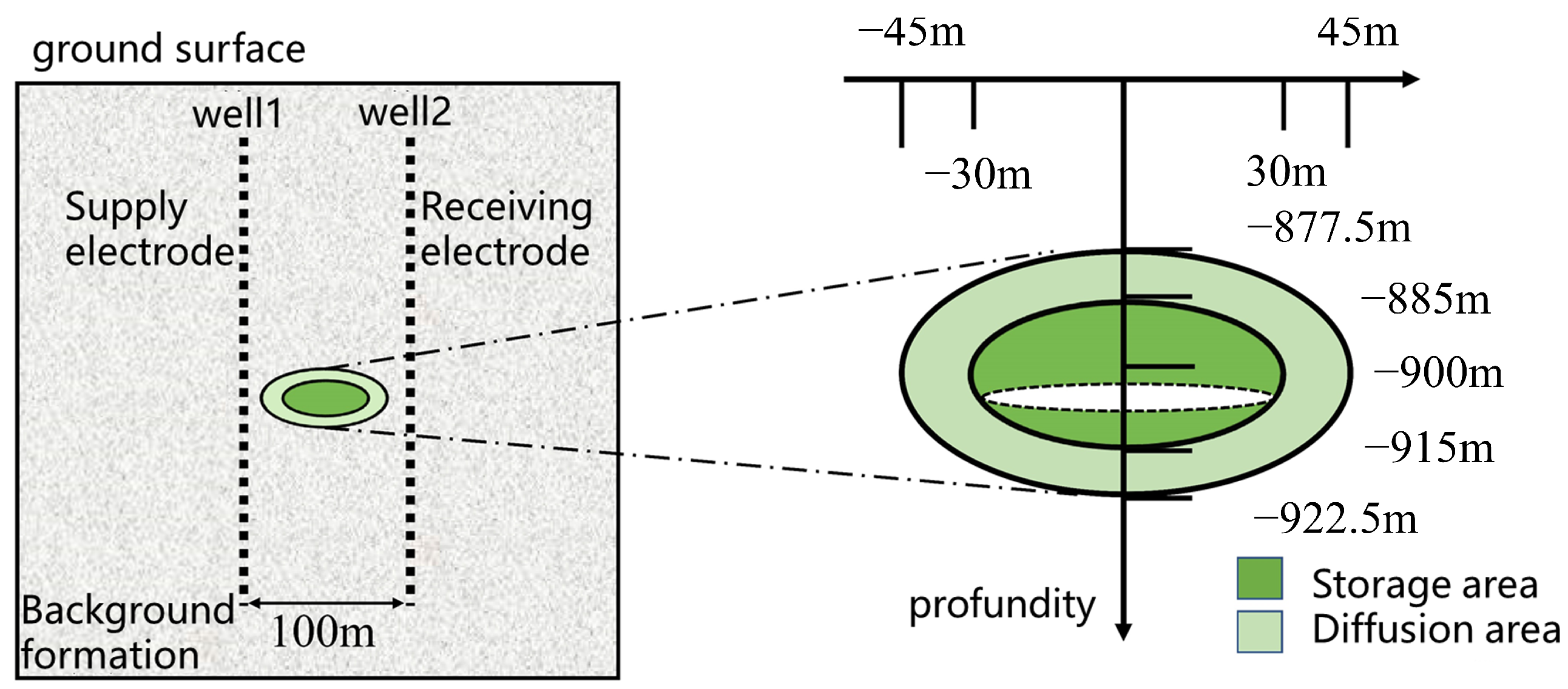
Therefore, this study establishes an inversion model for cross-borehole resistivity measurement (Figure 3). In the simulation process, the power supply electrode and receiving electrode are placed in observation wells 1 and 2, respectively. Typically, CO2 can reach a supercritical state at depths greater than 800 m; thus, we set the CO2 injection depth at 900 m. Notably, due to the cap rock’s barrier and the buoyancy of the gas, the injected CO2 typically forms a funnel-shaped distribution. To simplify this in the simulation, the CO2 injection zone is modeled as an ellipsoidal storage region with a constant aspect ratio, where variations in the ellipsoid sizes correspond to different volume ranges of the injected CO2. The electrodes are placed at depths between 800 m and 1000 m in two observation wells, located 50 m from the injection well, with the ellipsoidal storage region at the center. The power supply electrode in observation well 1 begins at a depth of 800 m and is moved downward in 10 m increments, while the potential values of the receiving electrode in observation well 2 are recorded. This results in a model with 21 × 21 apparent resistivity data points.
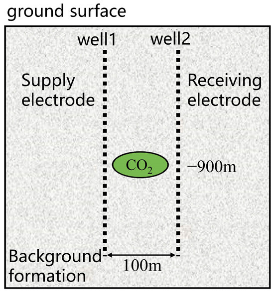
Figure 3.
Geometry of the CO2 inversion model. The ellipsoidal storage region is centered between the two wells, simulating the CO2 injection zone at a depth of 900 m.
To investigate the changes in resistivity inversion imaging under different parameter conditions, two models were established: a homogeneous half-space model (model A) and a horizontally layered two-layer model (model B) [44,45]. Simulations were conducted by varying the CO2 storage zone volume, resistivity, and background resistivity. Additionally, simulations of the resistivity changes in the storage zone during CO2 diffusion were carried out for inversion imaging analysis. The imaging results were obtained by varying different variables of the storage zone, allowing an analysis of how these parameters influence the resistivity values. In the inversion results, the resistivity difference represents the deviation between the inverted resistivity values and the model’s set resistivity values. A comparative analysis was then carried out to evaluate the discrepancies between the inversion results and the model parameters. The model parameter settings are summarized in Table 1.

Table 1.
Inversion model setup parameters.
4. Study of the Inversion Effect of Storage Zone Resistivity
4.1. Influence of Storage Zone Volume Changes on Imaging Results
4.1.1. Homogeneous Half-Space Model A1
As CO2 is continuously injected into the storage zone, the volume of the CO2 storage zone () increases. To assess the impact of these volume changes on the inverted resistivity results, the is varied at different stages of injection during the inversion process. The inversion results are presented in Figure 4.
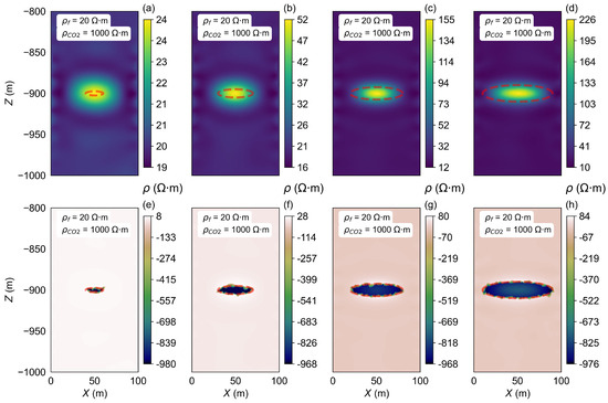
Figure 4.
Inversion results of different in model A1. (a–d) show the resistivity inversion results at different stages of CO2 injection. Images (e–h) display the differences between the inverted resistivity values and the model parameters set for each stage. The red elliptical dashed line indicates the predefined storage zone.
The inverted background resistivity results generally align with the model settings, the red elliptical dashed line indicates the predefined storage zone, and the inverted location and dimensions of the storage zone are completely consistent with the model settings. The resistivity difference in the background layer region (Figure 4e–h) also confirms both the location and size of the storage zone. For example, as depicted in Figure 4a, the major axis, minor axis, and focal length of the CO2 storage zone are set at 10 m, 10 m, and 2.5 m, respectively. When the resistivity of the CO2 storage zone () is set to 1000 ·m, the inverted resistivity range falls between 19 and 24 ·m. The inverted resistivity near the storage zone is approximately 24 ·m, while the surrounding resistivity is inverted to 19 ·m, which is lower than the background resistivity () of 20 ·m. This is attributed to the high-resistance characteristics of the high-resistance storage zone, which results in reduced current density in the surrounding area. The significant discrepancy between the inverted resistivity of the storage zone and the model-set resistivity is primarily due to the relatively small and the contrast.
The difference in resistivity results obtained through inversion effectively reflects the resistivity variations. As the increases, the inverted resistivity of the storage zone gradually increases, with substantial variations, indicating that the has a large impact on the inversion outcomes. Although the resistivity value of the storage zone is set to be a relatively high value, small storage volumes make it challenging to obtain accurate inversion results.
4.1.2. Horizontal Stratified Model B1
In most cases, the subsurface formations are typically horizontal and layered. To analyze the effect of varying on resistivity inversion under these conditions, a horizontal two-layer stratified model (model B1) is adopted. The model parameters used for this analysis are provided in Table 1. The inversion results for this model are shown in Figure 5.
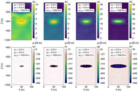
Figure 5.
Inversion results of the changes in model B. (a–d) show the resistivity inversion results at different stages of CO2 injection. Images (e–h) display the differences between the inverted resistivity values and the model parameters set for each stage.
For the horizontally layered model, when keeping the constant, as the CO2 injection volume increases, an increase in the CO2 injection volume leads to a gradual expansion of the storage zone. The inversion results, shown in Figure 5, clearly delineate the location and size of the storage zone, as indicated by the red dashed line. The inversion also reveals a clear horizontal layering effect, which is consistent with the accurate inversion of the background resistivity observed in model A1. As the increases, the inverted resistivity values of the storage zone gradually increase from 10 ·m to 95 ·m. This is approximately half of the value observed in model A1.
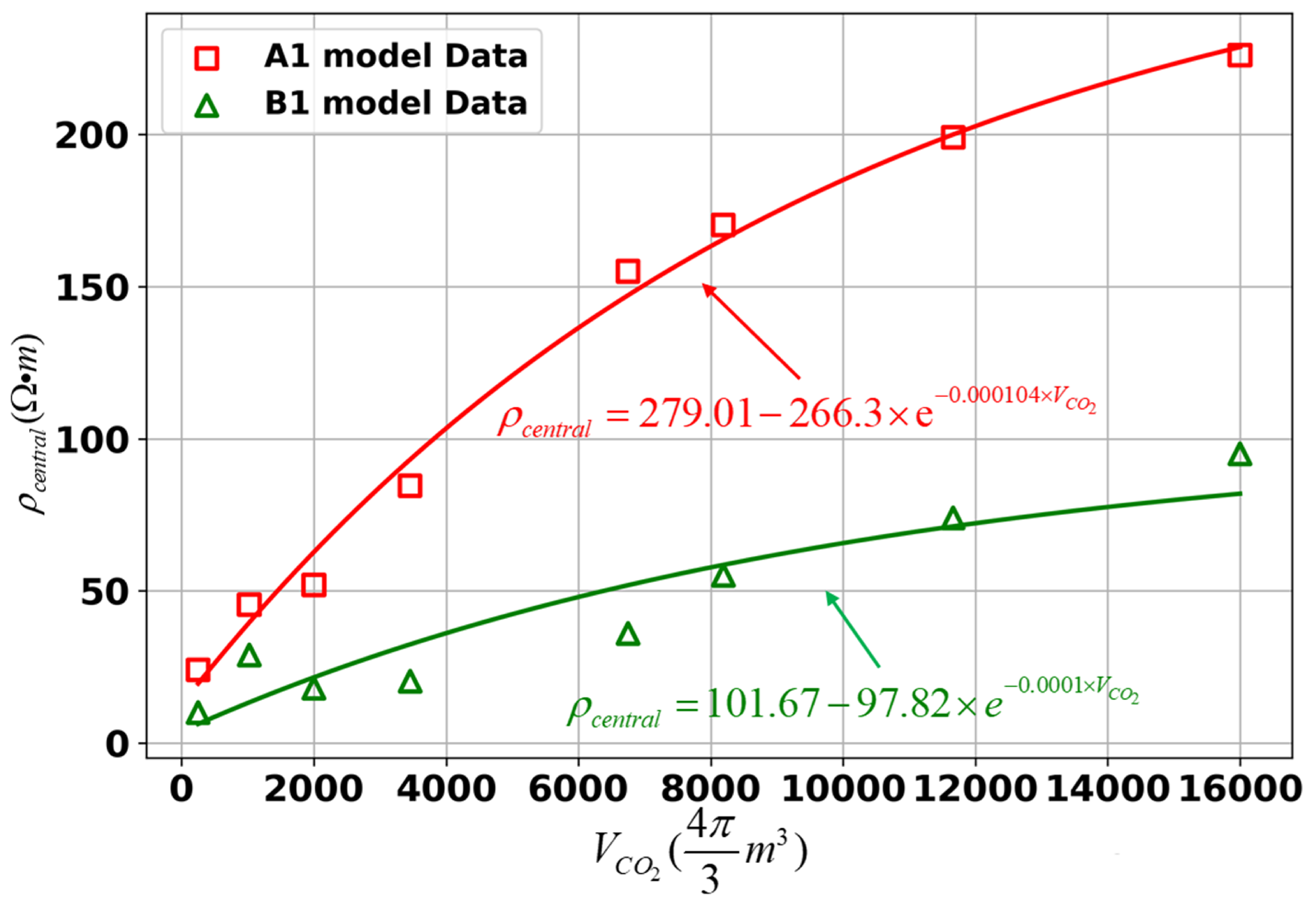
For both model A1 and model B1, we analyze the relationship between the and the inverted resistivity of the central storage zone (), i.e., the point of (50, −900) (Figure 6). The results indicate that, in both models, the increases as the increases. The fitting curves approximate exponential functions, with the growth rate of gradually decreasing as the increases. However, the rate of decrease slows down, and the ultimately approaches a stable value (e.g., approximately 279.01 ·m in model A1). Further research on this will be conducted in subsequent sections.
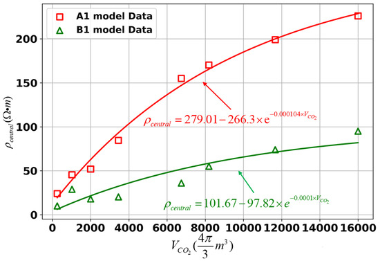
Figure 6.
Relationship between the and in point (50, −900) for different models. The corresponding lines represent the best-fit exponential functions.
4.2. Influence of Storage Zone Resistivity Changes on Imaging Results
4.2.1. Homogeneous Half-Space Model A2
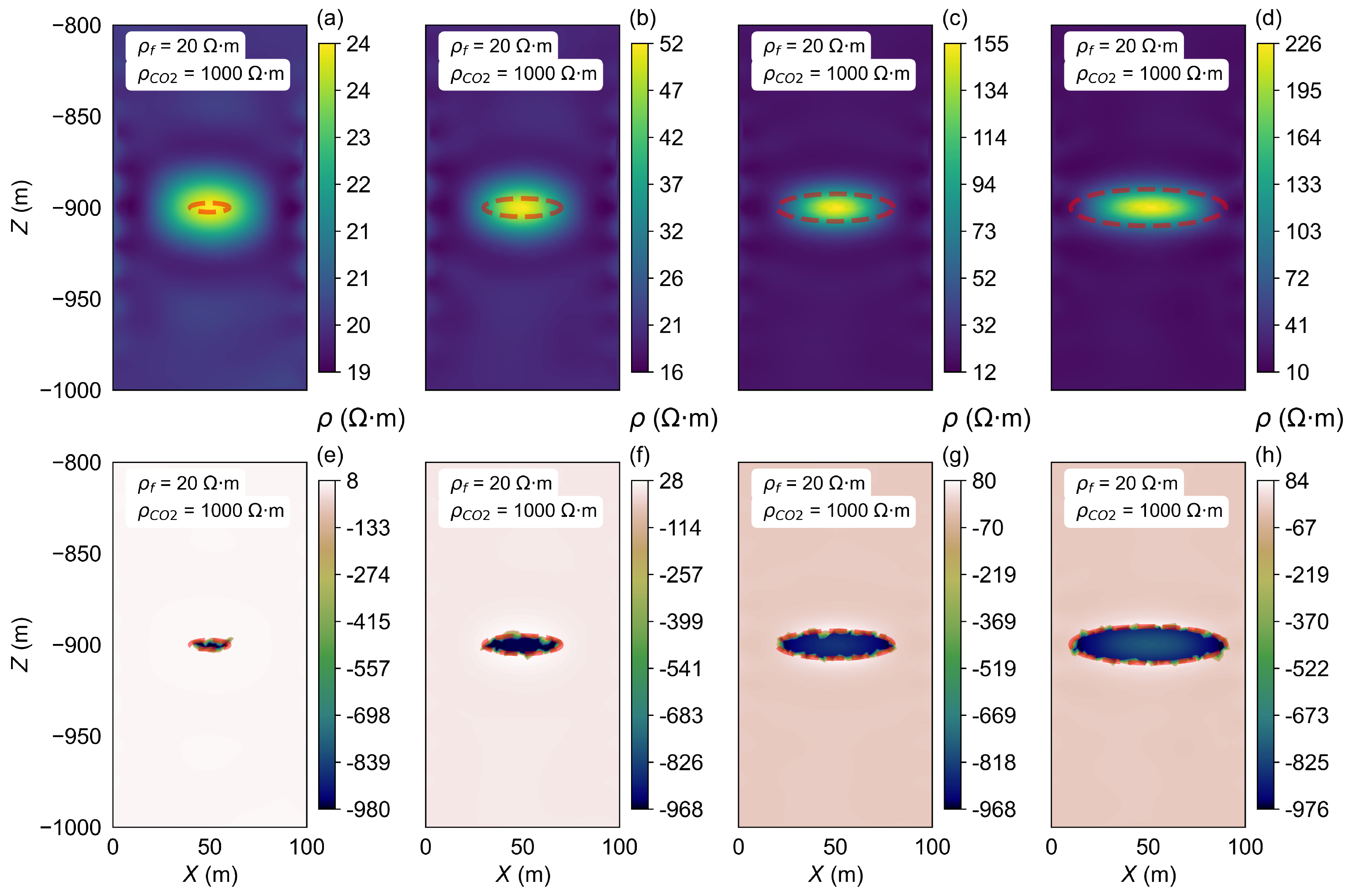
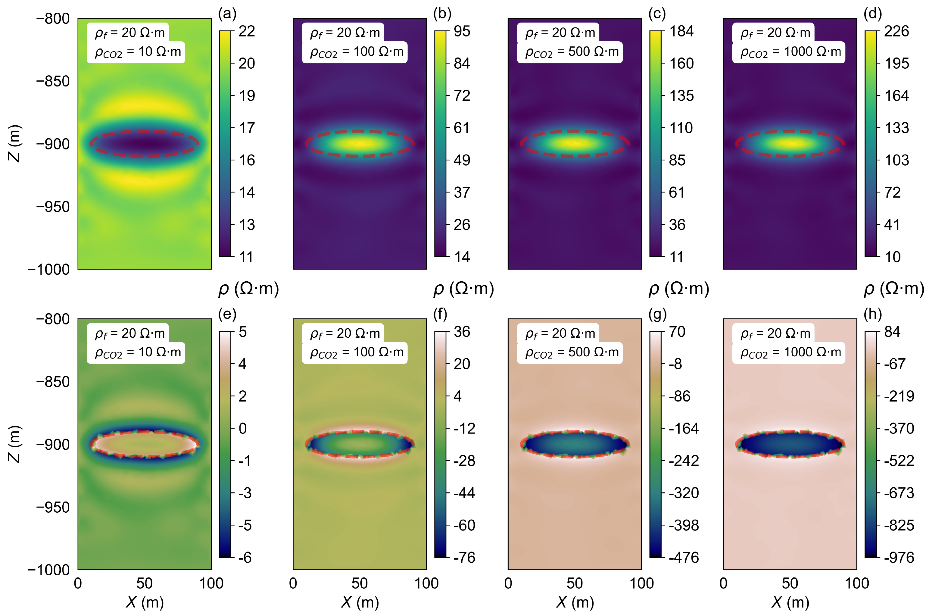
As the injection time increases, once the reaches the set maximum capacity, continued CO2 injection will cause significant changes in the resistivity within the storage zone. The inversion process was carried out for the homogeneous half-space model A2 to investigate this effect. The background resistivity was set to 20 ·m, while the semi-major axis, semi-minor axis, and focal length of the ellipsoidal CO2 storage zone were defined as 40 m, 40 m, and 10 m, respectively. Four sets of were considered, 10 ·m, 100 ·m, 500 ·m, and 1000 ·m, as outlined in the parameters presented in Table 1. The inversion results are shown in Figure 7.
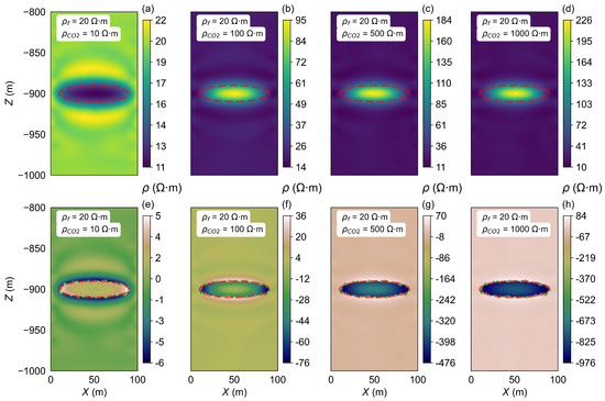
Figure 7.
Inversion results of the changes in model A2. (a–d) show the resistivity inversion results at different stages of CO2 injection. Images (e–h) display the differences between the inverted resistivity values and the model parameters set for each stage.
As CO2 continues to be injected into the storage zone, when keeping the constant, the gradually changes. This results in varying resistivity inversion images, as shown in Figure 7.
In Figure 7a, the resistivity of the storage zone is set to 10 ·m. The inverted resistivity of the CO2 storage zone inversion result close to 11 ·m and the surrounding areas have resistivity values close to 20 ·m, which matches the model’s parameters. However, a notable change occurs when the exceeds the . In this scenario, the resistivity inversion results become less accurate as the contrast between the storage zone and surrounding layers increases (Figure 7b–d). In Figure 7d, the is set to 1000 ·m, while the inverted resistivity of the storage zone resistivity is only 226 ·m. In all cases of the existence of the high-resistivity anomaly, the inverted resistivity results show a low-resistivity surrounding layer around the high-resistivity storage zone. The differences between the inversion results and the model settings are shown in Figure 7e–h, which can clearly reflect the individual impact of the storage zone on the inversion results. As the resistivity increases (from 10 ·m to 500 ·m), the difference becomes more pronounced.
In general, our results show that when the storage zone resistivity is much greater than the background resistivity, the inversion process may underestimate the resistivity in the storage zone, as the system’s electrical response becomes more sensitive to the larger resistivity contrast. This discrepancy leads to less precise inverted results, as demonstrated in the cases where the resistivity of the storage zone exceeds the background value significantly.
4.2.2. Horizontal Two-Layer Model B2
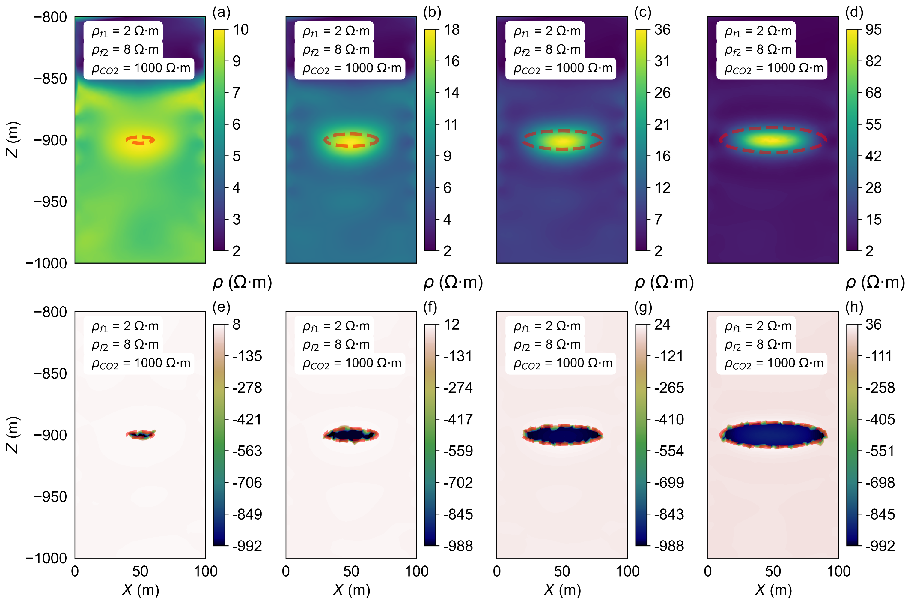
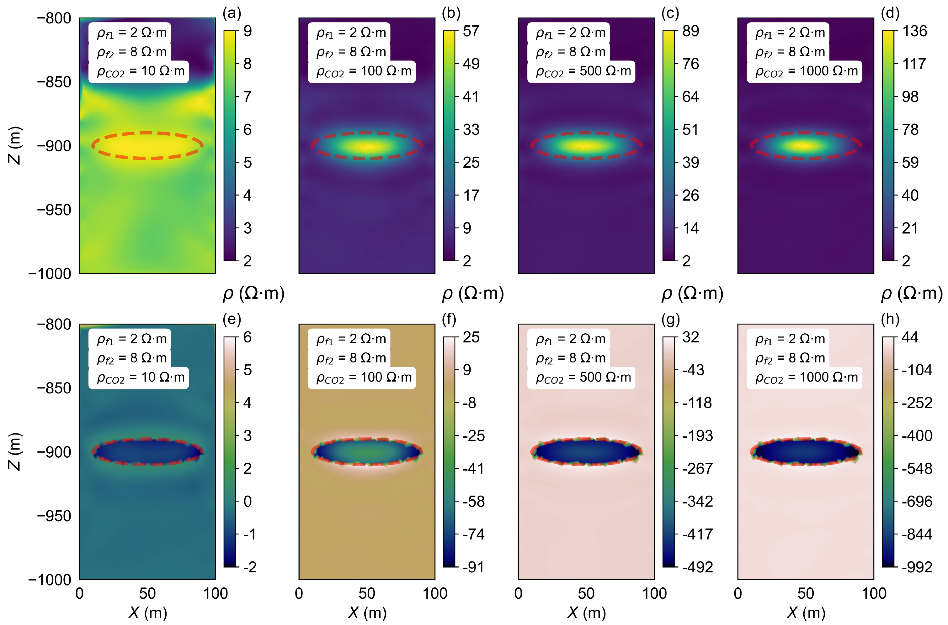
The horizontal two-layer model B2 was established, and the was changed, with values from 10 ·m to 1000 ·m. The inversion results are shown in Figure 8.
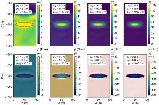
Figure 8.
Inversion results of the changes in model B2. (a–d) show the resistivity inversion results at different stages of CO2 injection. Images (e–h) display the differences between the inverted resistivity values and the model parameters set for each stage.
In contrast to the findings in model A1, where the storage zone resistivity can be accurately inverted to match the model parameters within a certain range, the results from model B2 indicate a different trend. Specifically, only when the is set to 10 ·m do the inversion results match the model’s set value of 10 ·m. As the increases, the inverted resistivity values gradually rise; however, even at the highest value of 1000 ·m, the inverted resistivity only reaches a maximum of 136 ·m, which is still significantly lower than the model’s set value of 1000 ·m.
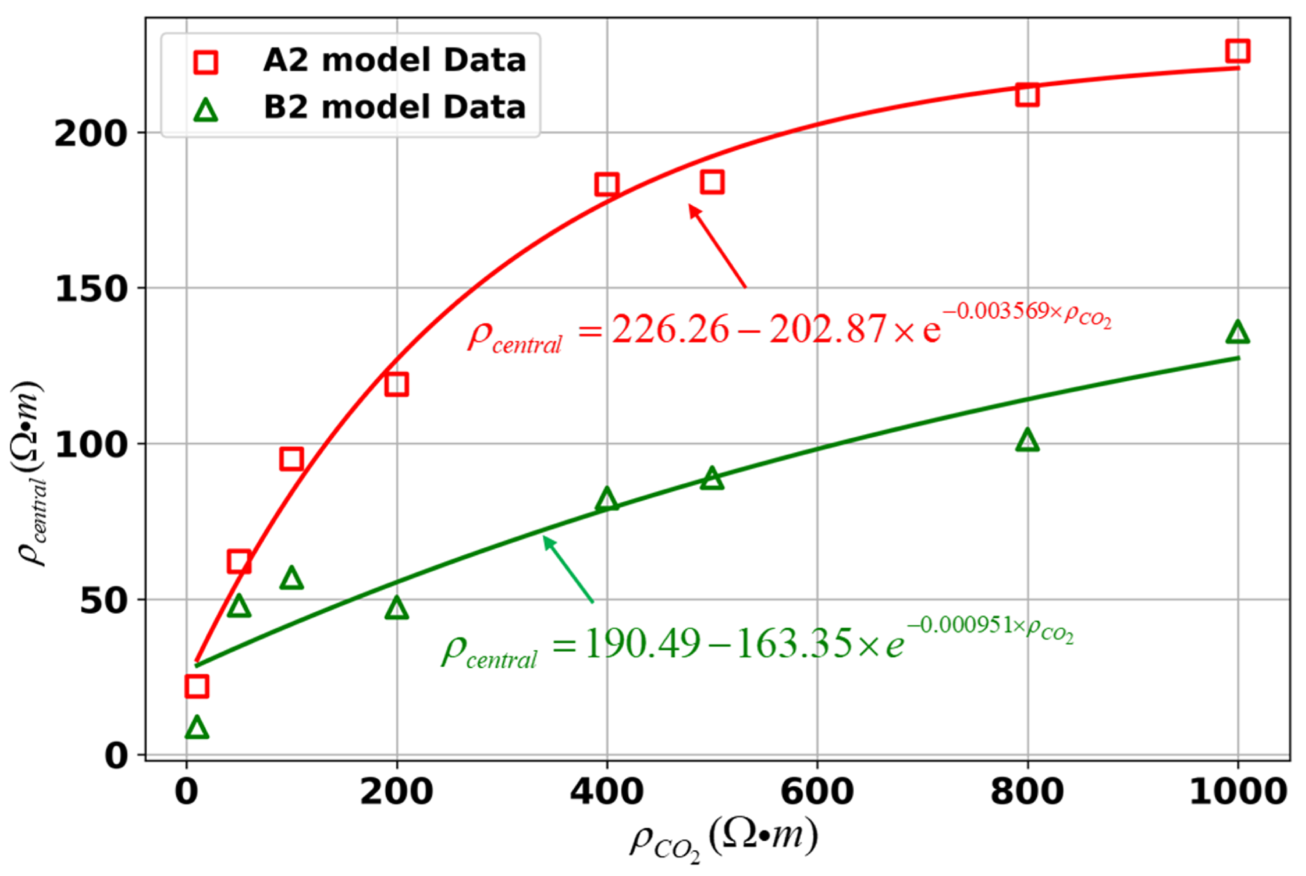
To further investigate the relationship between the and the in both models, fitting curves for different models were plotted as shown in Figure 9. The results indicate that, overall, as the increases, the also gradually increases. The fitting curves for both model A2 and model B2 approximate exponential functions. When only the is varied, a notable deviation between the central resistivity and the set values occurs, with this discrepancy becoming more pronounced as the increases.
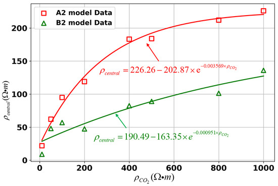
Figure 9.
Relationship between the and the for different models.
4.3. Impact of Background Resistivity Variations on Imaging Results
4.3.1. Homogeneous Half-Space Model A3
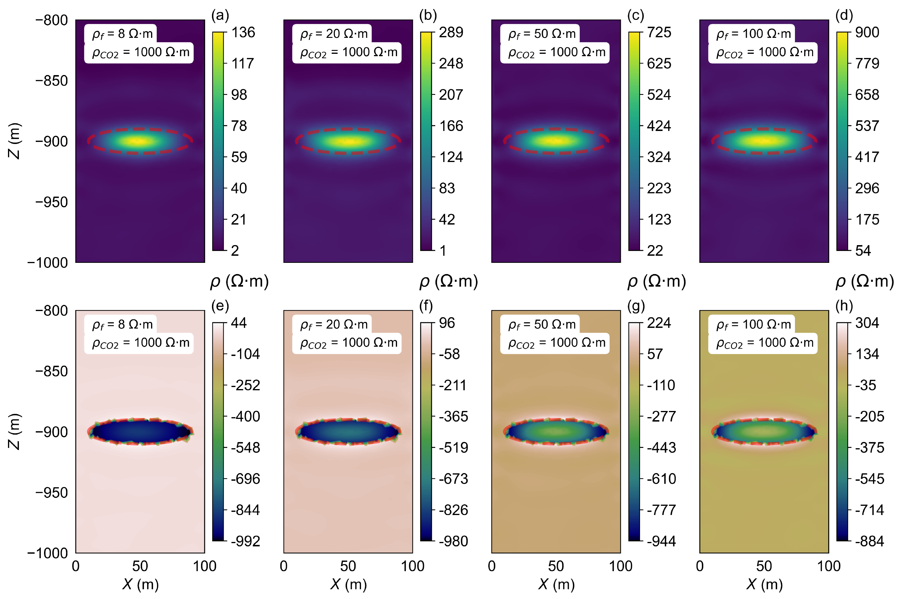
As mentioned above, we have discussed the effects of and variations on the inversion results. It was found that, compared to the uniform half-space model, the resistivity values from the inversion are significantly different in the horizontally layered model. This discrepancy could be due to the influence of the settings. Therefore, in this section, we will analyze the changes in inversion resistivity by altering the in model A3. The model parameters are set as shown in Table 1, and the inversion results are shown in Figure 10.
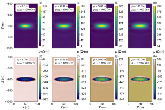
Figure 10.
Inversion results of the changes in model A3. (a–d) show the resistivity inversion results at different stages of CO2 injection. Images (e–h) display the differences between the inverted resistivity values and the model parameters set for each stage.
In all four cases, the is set differently, but the resistivity difference in the background region is close to 0, indicating that the inverted background resistivity matches the model parameters. The position and size of the storage zone obtained from the inversion are in perfect agreement with the model settings. Since the is relatively low, the inverted resistivity of the high-resistance storage zone is also lower. Figure 10e–h show that as the increases, the resistivity difference also increases, reflecting similar trends to the inverted resistivity values.
The discrepancy between the inverted resistivity and the model settings in the high-resistance storage zone is mainly attributed to the influence of the . When the is increased to 100 ·m, the change in the inverted storage zone resistivity is relatively small. This suggests that once the reaches a certain threshold, its impact tends to stabilize.
4.3.2. Horizontal Two-Layered Model B3
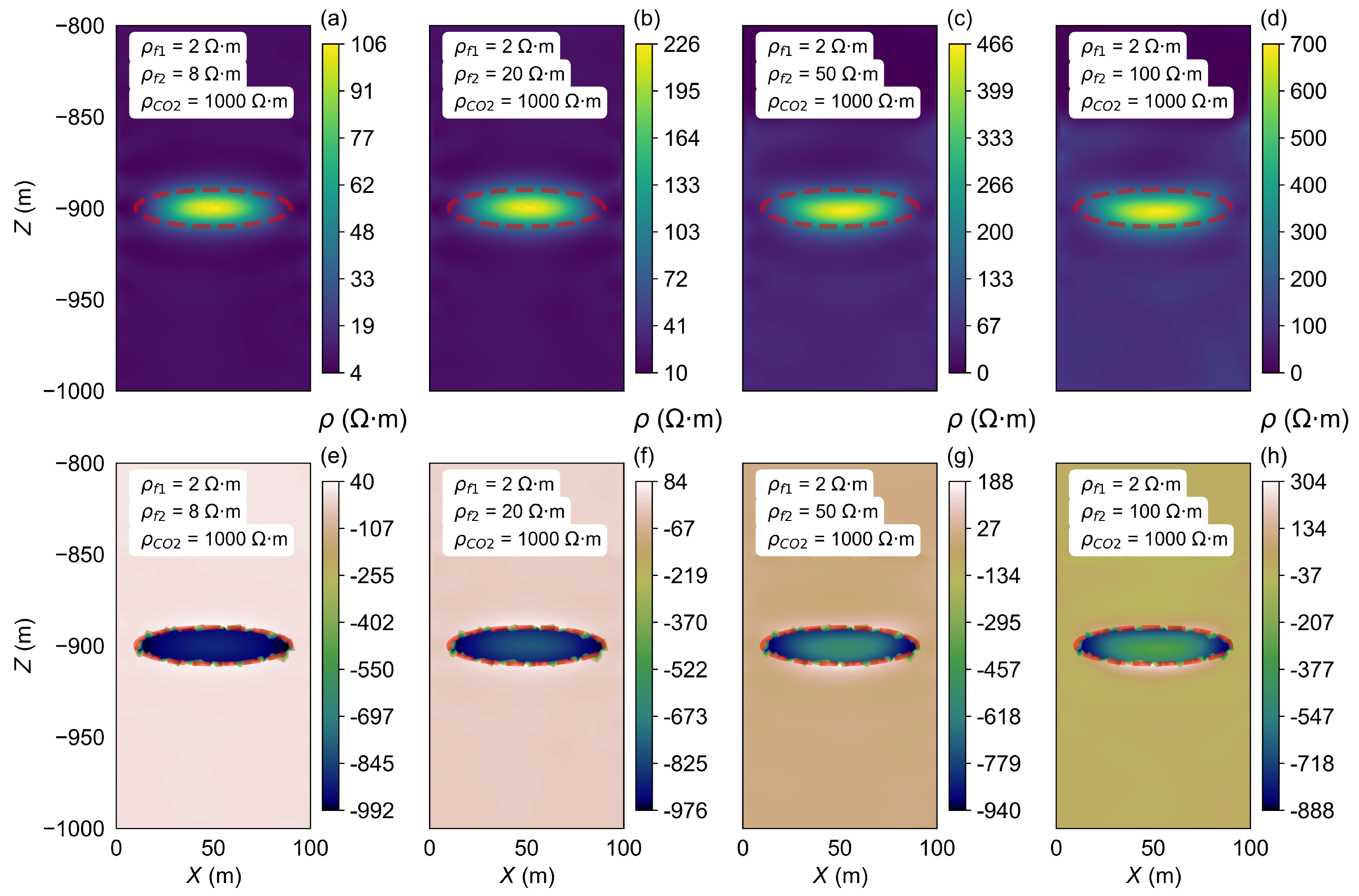
Typically, the cap layer of a CO2 storage zone consists of low-resistivity rock structures, which are better for geological storage. Therefore, in this study of the horizontal model B3, the resistivity of the first layer (cap layer) remains constant, and only the resistivity of the second layer (storage layer) is varied.
Similarly, the location of the storage zone is accurately reflected. Moreover, the background resistivity is correctly inverted in all four models. As the increases, the inverted resistivity of the storage zone continues to show a consistently high growth trend. Compared to model A3, the inverted resistivity values for model B3 are lower. This is because the presence of the first low-resistivity layer causes the current density in the storage zone to be relatively sparse, leading to lower potential in the forward modeling process (see Figure 11).
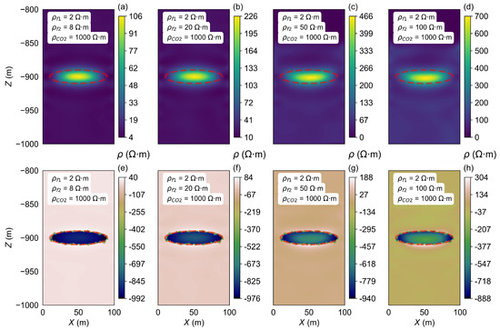
Figure 11.
Inversion results of the changes in model B3. (a–d) show the resistivity inversion results at different stages of CO2 injection. Images (e–h) display the differences between the inverted resistivity values and the model parameters set for each stage.
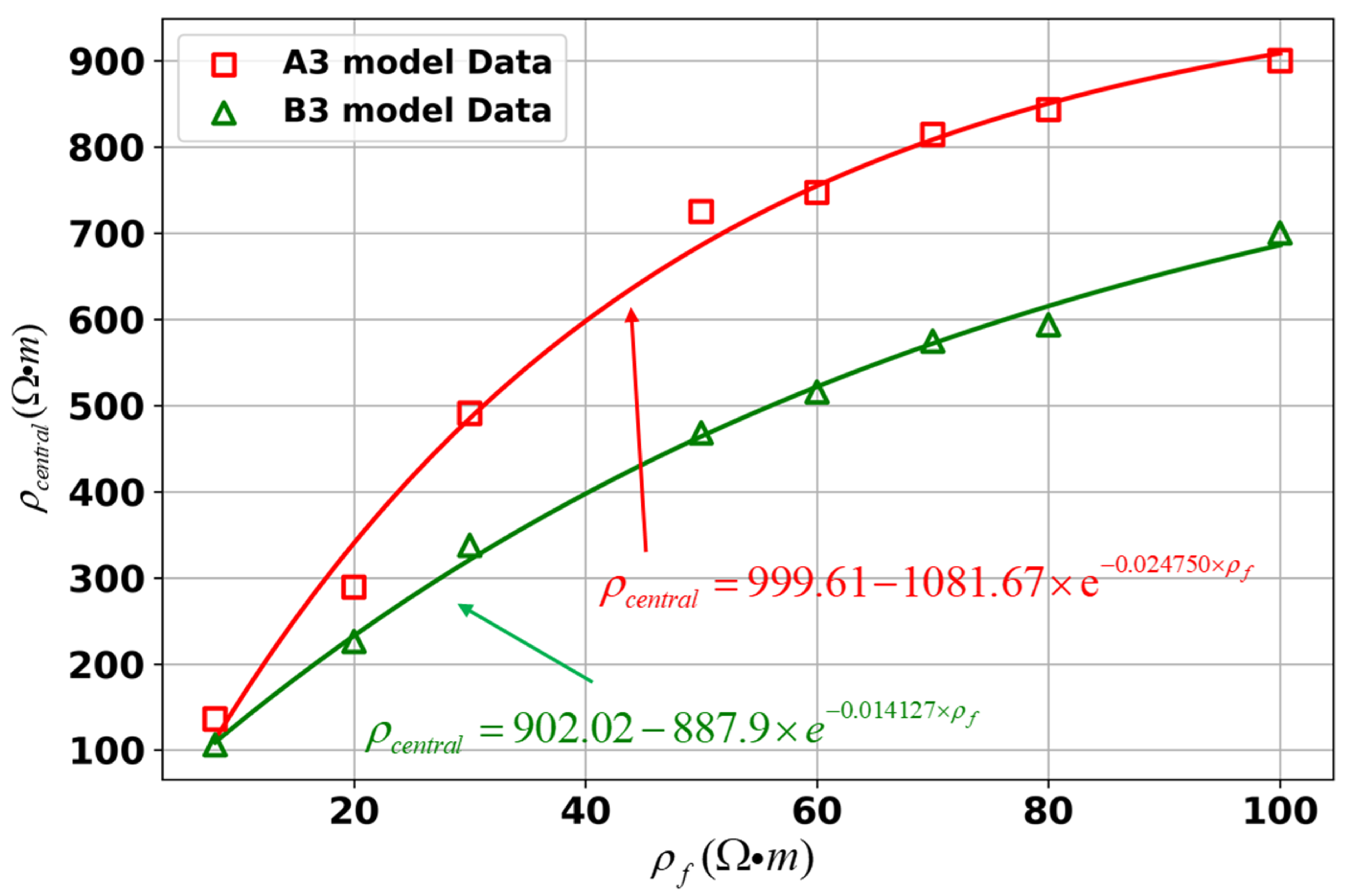
By analyzing the variations in both models under different conditions, as shown in Figure 12, it is further demonstrated that changes in the influence the inversion results. Under model A3 conditions, the inverted resistivity ultimately converges to 999.61 ·m, which is very close to the set CO2 resistivity of 1000 ·m. Similarly, model B3 reaches a final resistivity of 902.02 ·m. These results indicate that the is a key factor affecting the inversion resistivity distribution.
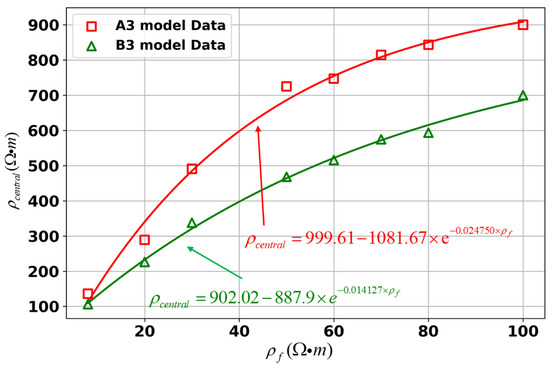
Figure 12.
Relationship between the and the for different models.
From the analysis of the three factors—storage zone volume, resistivity, and background resistivity—it is found that the impact of background resistivity on the inversion result is greater than the impact of storage zone resistivity, which, in turn, is greater than the impact of storage zone volume. This finding underscores the importance of conducting a thorough pre-analysis of the background strata prior to monitoring the CO2 injection and storage process in practical CO2 sequestration operations.
4.4. Study on the Impact of CO2 Diffusion on Imaging Results
As the CO2 injection time increases, the CO2 content in the storage zone gradually increases, and the volume occupied by CO2 expands. Once CO2 is completely distributed within the storage zone, the resistivity will gradually decrease. The changes in resistivity during this process, as discussed earlier, are due to the injection of CO2 as a high-pressure gas, which alters the elastic properties of the reservoir. CO2 will diffuse to some extent, and this diffusion will affect the properties of the subsurface region as well as surface water, potentially posing risks to both the ecosystem and human activities. Therefore, it is essential to closely analyze the CO2 diffusion process and its implications for the monitoring and safety of CO2 sequestration operations.
In the previous model, the ratio of the semi-axes of the elliptical storage zone was 4:4:1, with a relatively small width in the vertical direction (z-axis). To improve the inversion performance in the vertical direction, the semi-axis ratio of the elliptical shape is set to 2:2:1 for the CO2 diffusion simulation. This change allows for a more representative model of the CO2 diffusion within the subsurface, ensuring better spatial resolution in the vertical dimension, which is critical for assessing the behavior of CO2 as it migrates within the geological formations.
The simulation assumes that no diffusion occurs during the initial injection stage, where the CO2 volume is still low. Diffusion is set to begin only after the storage zone is fully filled with CO2. In this model, the semi-axes of the small elliptical storage zone are set to 30 m, 30 m, and 15 m, and these values are kept constant throughout the simulation. These dimensions represent the storage zone before diffusion begins, and they reflect the typical spatial extent of CO2 accumulation in the initial stages of injection. Once diffusion begins, the diffusion area is defined by a larger elliptical shape, with semi-axes set to 45 m, 45 m, and 22.5 m, corresponding to the maximum extent of CO2 distribution. The region between the small and large ellipses is designated as the diffusion zone, as illustrated in Figure 13. This area represents the region where CO2 gradually spreads from the initial storage zone into the surrounding rock formations. The rate of resistivity change within the diffusion zone depends on factors such as the rate of CO2 injection, the permeability of the rock, and the diffusion characteristics of CO2 in the subsurface. To simplify, the diffusion process is modeled by gradually reducing the resistivity in this zone, as CO2 replaces the air or water that was originally present in the pore spaces of the geological formations. The resistivity of the diffusion area is set as follows according to Figure 13:

Figure 13.
CO2 diffusion model geometry. The smaller ellipse represents the storage zone and the larger ellipse indicates the diffusion zone.
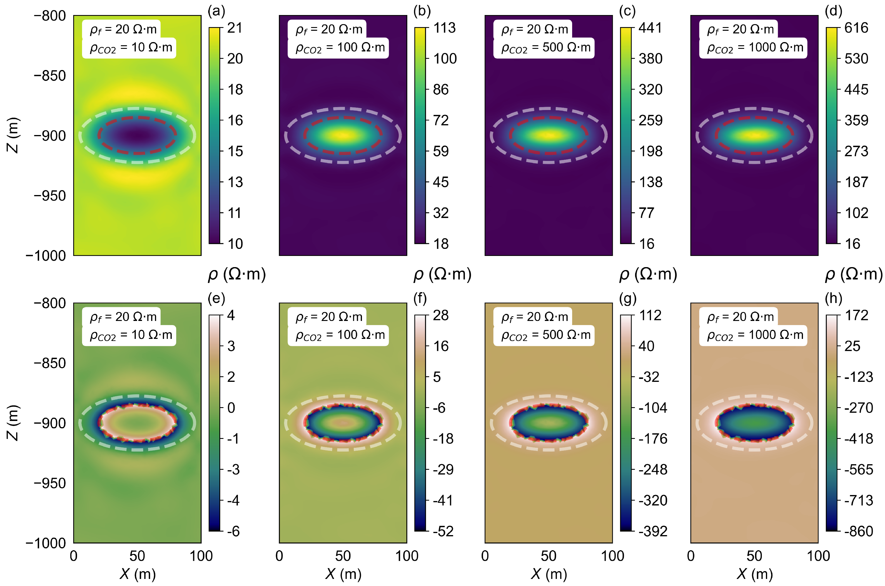
During the CO2 diffusion process, with the storage volume held constant, the resistivity inversion results are analyzed for different injection periods (i.e., varying resistivity of the CO2 storage and diffusion zone). First, the homogeneous half-space model A4 is established, with the set at 10, 100, 500, and 1000 ·m, and the resistivity of the diffusion zone set at 19, 28, 68, and 118 ·m.
Figure 14 shows the inversion results after diffusion. As the increases, the inversion results show corresponding changes. However, it is challenging to directly distinguish the differences in the diffusion zone’s range from the inversion results alone. To further investigate the impact of diffusion on the inversion results, the differences between the inverted resistivity after diffusion and the initial model before diffusion (which can be measured before CO2 injection) are calculated (Figure 14e–h). By comparing the inversion results to the initial model settings, we can observe that significant layering appears in the resistivity values of both the sequestration and diffusion zones, as indicated by the areas marked by white dashed and red dashed lines. For example, Figure 14h shows a significant increase in the resistivity difference before and after diffusion. This is because the diffusion zone resistivity of 118 ·m is much higher than the model’s initial settings. The resistivity difference in the diffusion zone is close to 118 ·m, enabling an accurate identification of the diffusion region and its corresponding resistivity values.
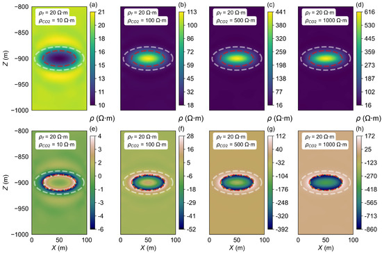
Figure 14.
Inversion results of changing the storage area when CO2 diffuses in model A4. (a–d) show the resistivity inversion results at different stages of CO2 injection. Images (e–h) display the differences between the inverted resistivity values and the model parameters set for each stage. The red elliptical dashed line indicates the location of the storage zone, and the area between the red dashed line and the white elliptical dashed line represents the diffusion zone.
The difference results highlight the effects of CO2 diffusion on the resistivity distribution, allowing for a more accurate identification of the diffusion region and providing deeper insights into the impact of CO2 on subsurface resistivity. This analysis emphasizes the importance of considering diffusion effects when monitoring CO2 sequestration and tracking plume migration in real-world applications.
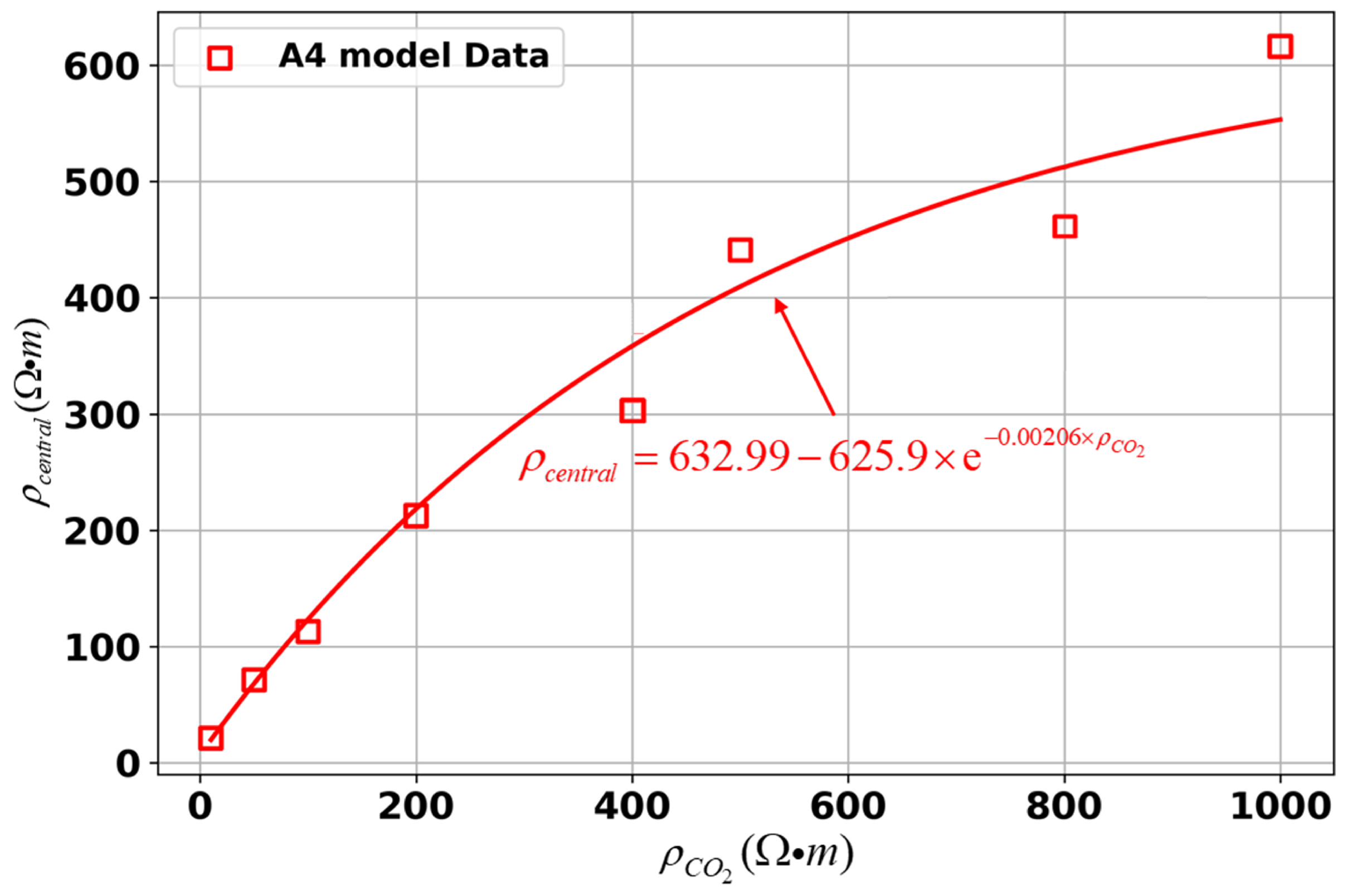
We also analyze the variation in the under diffusion conditions for both models, as shown in Figure 15. The background resistivity plays a key role in influencing the diffusion behavior and, consequently, the resistivity inversion results. However, overall, under diffusion conditions, the increases as the resistivity of the sequestration zone increases, verifying the accuracy of the inversion. The increase in under diffusion conditions is consistent with the expectation that CO2 injection reduces the due to the displacement of pore fluids by CO2. As the diffusion process progresses, the injected CO2 gradually fills the storage zone, leading to a redistribution of resistivity.
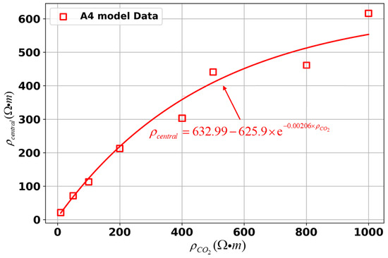
Figure 15.
Relationship between the and the for different models under diffusion conditions.
5. Conclusions
This study employs the IGN method to examine the resistivity inversion of CO2 sequestration zones using cross-borehole measurements. We constructed two geological models—a homogeneous half-space model and a horizontally layered model—to evaluate the impacts of storage zone volume, storage zone resistivity, background resistivity, and CO2 diffusion on inversion results. Increasing storage zone volume directly correlates with a rise in inverted resistivity; however, as volume grows, the rate of increase slows and stabilizes at a specific value, reflecting a size-dependent limit. The resistivity of the storage zone significantly influences inversion accuracy; reliable outcomes are achieved within a defined range (e.g., below 100 ·m in the homogeneous model), but when this threshold is exceeded, substantial deviations occur, with errors escalating as resistivity rises further. Background resistivity variations notably affect inversion results, particularly in high-resistivity zones, though this effect plateaus beyond a saturation point slightly above 100 ·m, beyond which additional increases have minimal impact. When CO2 diffusion is introduced, a distinct transition zone emerges between the storage and background layers. Following CO2 injection, resistivity decreases in both the storage and diffusion zones, driving pronounced changes in the inverted resistivity. Comparisons of pre- and post-injection data enable clear identification of the diffusion zone, enhancing tracking capabilities. This study thus provides a reliable approach to ensuring the safety and stability of CO2 storage operations, with practical implications for optimizing long-term sequestration strategies.
Author Contributions
Conceptualization, C.W. and T.Y.; methodology, C.W., T.L. and T.Y.; resources, C.W., X.F., and Y.Y.; software, C.W., T.Y., X.F. and H.L.; visualization, C.W. and T.Y.; writing—original draft preparation, C.W. and T.Y.; writing—review and editing, T.L.; project administration, T.L.; supervision, T.L. and B.D.; validation, L.Y. and Y.L. All authors have read and agreed to the published version of the manuscript.
Funding
This workwas supported by the National Natural Science Foundation of China (No. 42204058), the Natural Science Foundation of Chongqing (CSTB2024NSCQ-LZX0011 and CSTB2023NSCQ-MSX1050), the National Nonprofit Institute Research Grant of IGGE (No. AS2024J02), and the Central Universities Basic Research Operating Expenses (2024CDJCGJ-013).
Institutional Review Board Statement
Not applicable.
Informed Consent Statement
Not applicable.
Data Availability Statement
Data are contained within the article.
Conflicts of Interest
The authors declare no conflicts of interest.
References
- Khachoo, Y.H.; Cutugno, M.; Robustelli, U.; Pugliano, G. Impact of Land Use and Land Cover (LULC) Changes on Carbon Stocks and Economic Implications in Calabria Using Google Earth Engine (GEE). Sensors 2024, 24, 5836. [Google Scholar] [CrossRef] [PubMed]
- Bosch, D.; Ledo, J.; Queralt, P.; Bellmunt, F.; Luquot, L.; Gouze, P. Core-Scale Electrical Resistivity Tomography (ERT) Monitoring of CO2–Brine Mixture in Fontainebleau Sandstone. J. Appl. Geophys. 2016, 130, 23–36. [Google Scholar] [CrossRef]
- Shashkin, P.; Gurevich, B.; Yavuz, S.; Glubokovskikh, S.; Pevzner, R. Monitoring Injected CO2 Using Earthquake Waves Measured by Downhole Fibre-Optic Sensors: CO2CRC Otway Stage 3 Case Study. Sensors 2022, 22, 7863. [Google Scholar] [CrossRef] [PubMed]
- Chen, Y.J.; Wang, H.Y.; Sharma, M. The Benefits and Challenges of Well Monitoring of Gulong Shale Oil. Earth Energy Sci. 2025, in press. [Google Scholar] [CrossRef]
- De Giorgi, L.; Barbolla, D.F.; Torre, C.; Settembrini, S.; Leucci, G. Evaluation of a Ground Subsidence Zone in an Urban Area Using Geophysical Methods. Sensors 2024, 24, 3757. [Google Scholar] [CrossRef]
- Daily, W.; Owen, E. Cross-borehole Resistivity Tomography. Geophysics 1991, 56, 1228–1235. [Google Scholar] [CrossRef]
- Garcia, M.M.; Sattar, M.A.; Atmani, H.; Legendre, D.; Babout, L.; Schleicher, E.; Hampel, U.; Portela, L.M. Towards Tomography-Based Real-Time Control of Multiphase Flows: A Proof of Concept in Inline Fluid Separation. Sensors 2022, 22, 4443. [Google Scholar] [CrossRef]
- Acosta, J.A.; Gabarrón, M.; Martínez-Segura, M.; Martínez-Martínez, S.; Faz, Á.; Pérez-Pastor, A.; Gómez-López, M.D.; Zornoza, R. Soil Water Content Prediction Using Electrical Resistivity Tomography (ERT) in Mediterranean Tree Orchard Soils. Sensors 2022, 22, 1365. [Google Scholar] [CrossRef]
- Loke, M.H.; Chambers, J.E.; Rucker, D.F.; Kuras, O.; Wilkinson, P.B. Recent Developments in the Direct-Current Geoelectrical Imaging Method. J. Appl. Geophys. 2013, 95, 135–156. [Google Scholar] [CrossRef]
- Azffri, S.L.; Ibrahim, M.F.; Gödeke, S.H. Electrical Resistivity Tomography and Induced Polarization Study for Groundwater Exploration in the Agricultural Development Areas of Brunei Darussalam. Environ. Earth Sci. 2022, 81, 233. [Google Scholar] [CrossRef]
- Rubin, Y.; Hubbard, S.S.; Singh, V.P. (Eds.) Hydrogeophysics; Water Science and Technology Library; Springer: Dordrecht, The Netherlands, 2005; Volume 50. [Google Scholar] [CrossRef]
- Held, S.; Schill, E.; Pavez, M.; Díaz, D.; Muñoz, G.; Morata, D.; Kohl, T. Resistivity Distribution from Mid-Crustal Conductor to near-Surface across the 1200 Km Long Liquiñe-Ofqui Fault System, Southern Chile. Geophys. J. Int. 2016, 207, 1387–1400. [Google Scholar] [CrossRef]
- Chen, B.; Abascal, J.F.P.J.; Soleimani, M. Extended Joint Sparsity Reconstruction for Spatial and Temporal ERT Imaging. Sensors 2018, 18, 4014. [Google Scholar] [CrossRef]
- Lochbühler, T.; Breen, S.J.; Detwiler, R.L.; Vrugt, J.A.; Linde, N. Probabilistic Electrical Resistivity Tomography of a CO2 Sequestration Analog. J. Appl. Geophys. 2014, 107, 80–92. [Google Scholar] [CrossRef]
- Breen, S.J.; Carrigan, C.R.; LaBrecque, D.J.; Detwiler, R.L. Bench-Scale Experiments to Evaluate Electrical Resistivity Tomography as a Monitoring Tool for Geologic CO2 Sequestration. Int. J. Greenh. Gas Control 2012, 9, 484–494. [Google Scholar] [CrossRef]
- Nakatsuka, Y.; Xue, Z.; Garcia, H.; Matsuoka, T. Experimental Study on CO2 Monitoring and Quantification of Stored CO2 in Saline Formations Using Resistivity Measurements. Int. J. Greenh. Gas Control 2010, 4, 209–216. [Google Scholar] [CrossRef]
- Jia, N.; Wu, C.; He, C.; Lv, W.; Ji, Z.; Xing, L. Cross-Borehole ERT Monitoring System for CO2 Geological Storage: Laboratory Development and Validation. Energies 2024, 17, 710. [Google Scholar] [CrossRef]
- Al Hagrey, S.A. 2D Optimized Electrode Arrays for Borehole Resistivity Tomography and CO2 Sequestration Modelling. Pure Appl. Geophys. 2012, 169, 1283–1292. [Google Scholar] [CrossRef]
- Weinzierl, W.; Ganzer, M.; Rippe, D.; Lueth, S.; Schmidt-Hattenberger, C. Processed Seismic Data and ERT Inversion Models Used in the Estimation of Injected Masses for the Ketzin CO2 Pilot Project for the Years 2009 and 2012. 2021. Available online: https://dataservices.gfz-potsdam.de/panmetaworks/showshort.php?id=583837b5-a348-11eb-9603-497c92695674 (accessed on 11 March 2025).
- Alumbaugh, D.; Wilt, M.; Nichols, E.; Um, E.; Macquet, M.; Lawton, D.C.; Rippe, D.; Key, K.; Myer, D. ERT and Crosswell EM Imaging of CO2: Examples from a Shallow Injection Experiment at the Carbon Management Canada CaMI FRS in Southeast Alberta, Canada. In Proceedings of the Second International Meeting for Applied Geoscience & Energy, Houston, TX, USA, 28 August–1 September 2022; pp. 3107–3110. [Google Scholar] [CrossRef]
- Farzamian, M.; Blanchy, G.; McLachlan, P.; Vieira, G.; Esteves, M.; de Pablo, M.A.; Triantafilis, J.; Lippmann, E.; Hauck, C. Advancing Permafrost Monitoring With Autonomous Electrical Resistivity Tomography (A-ERT): Low-Cost Instrumentation and Open-Source Data Processing Tool. Geophys. Res. Lett. 2024, 51, e2023GL105770. [Google Scholar] [CrossRef]
- Sejati, P.A.; Saito, N.; Prayitno, Y.A.K.; Tanaka, K.; Darma, P.N.; Arisato, M.; Nakashima, K.; Takei, M. On-Line Multi-Frequency Electrical Resistance Tomography (mfERT) Device for Crystalline Phase Imaging in High-Temperature Molten Oxide. Sensors 2022, 22, 1025. [Google Scholar] [CrossRef]
- Li, X.; Li, Q.; Bai, B.; Wei, N.; Yuan, W. The Geomechanics of Shenhua Carbon Dioxide Capture and Storage (CCS) Demonstration Project in Ordos Basin, China. J. Rock Mech. Geotech. Eng. 2016, 8, 948–966. [Google Scholar] [CrossRef]
- Vilamajó, E.; Queralt, P.; Ledo, J.; Marcuello, A. Feasibility of Monitoring the Hontomín (Burgos, Spain) CO2 Storage Site Using a Deep EM Source. Surv. Geophys. 2013, 34, 441–461. [Google Scholar] [CrossRef]
- Bergmann, P.; Schmidt-Hattenberger, C.; Labitzke, T.; Wagner, F.M.; Just, A.; Flechsig, C.; Rippe, D. Fluid Injection Monitoring Using Electrical Resistivity Tomography—Five Years of CO2 Injection at Ketzin, Germany. Geophys. Prospect. 2017, 65, 859–875. [Google Scholar] [CrossRef]
- Schmidt-Hattenberger, C.; Bergmann, P.; Bösing, D.; Labitzke, T.; Möller, M.; Schröder, S.; Wagner, F.; Schütt, H. Electrical Resistivity Tomography (ERT) for Monitoring of CO2 Migration—From Tool Development to Reservoir Surveillance at the Ketzin Pilot Site. Energy Procedia 2013, 37, 4268–4275. [Google Scholar] [CrossRef]
- Wagner, F.M.; Wiese, B.U. Fully Coupled Inversion on a Multi-Physical Reservoir Model—Part II: The Ketzin CO2 Storage Reservoir. Int. J. Greenh. Gas Control 2018, 75, 273–281. [Google Scholar] [CrossRef]
- M, J.; Rippe, D.; Romdhane, A.; Schmidt-Hattenberger, C. CO2 Monitoring At The Ketzin Pilot Site With Joint Inversion: Application To Synthetic And Real Data. In Proceedings of the Fifth CO2 Geological Storage Workshop. European Association of Geoscientists & Engineers, Utrecht, The Netherlands, 21–23 November 2018; Volume 2018, pp. 1–5. [Google Scholar] [CrossRef]
- Li, T.; Gu, Y.J.; Lawton, D.C.; Gilbert, H.; Macquet, M.; Savard, G.; Wang, J.; Innanen, K.A.; Yu, N. Monitoring CO2 Injection at the CaMI Field Research Station Using Microseismic Noise Sources. J. Geophys. Res. Solid Earth 2022, 127, e2022JB024719. [Google Scholar] [CrossRef]
- Macquet, M.; Lawton, D.C.; Rippe, D.; Schmidt-Hattenberger, C. Semi-Continuous Electrical Resistivity Tomography Monitoring for CO2 Injection at the CaMI Field Research Station, Newell County, Alberta, Canada. In First International Meeting for Applied Geoscience & Energy Expanded Abstracts; SEG Technical Program Expanded Abstracts; Society of Exploration Geophysicists: Houston, TX, USA, 2021; pp. 362–366. [Google Scholar] [CrossRef]
- Macquet, M.; Lawton, D.C.; Isaac, H.J. Ambient Noise Correlation Study at the CaMI Field Research Station CO2 Injection Pilot Site, Newell County, Alberta, Canada. In Proceedings of the SEG International Exposition and Annual Meeting, OnePetro, Online, 11–16 October 2020. [Google Scholar] [CrossRef]
- Raab, T.; Weinzierl, W.; Wiese, B.; Rippe, D.; Schmidt-Hattenberger, C. Development of an Electrical Resistivity Tomography Monitoring Concept for the Svelvik CO2 Field Lab, Norway. In Advances in Geosciences; Copernicus GmbH: Göttingen, Germany, 2020; Volume 54, pp. 41–53. [Google Scholar] [CrossRef]
- Wilkinson, P.B.; Loke, M.H.; Meldrum, P.I.; Chambers, J.E.; Kuras, O.; Gunn, D.A.; Ogilvy, R.D. Practical Aspects of Applied Optimized Survey Design for Electrical Resistivity Tomography. Geophys. J. Int. 2012, 189, 428–440. [Google Scholar] [CrossRef]
- Cubbage, B.; Noonan, G.E.; Rucker, D.F. A Modified Wenner Array for Efficient Use of Eight-Channel Resistivity Meters. Pure Appl. Geophys. 2017, 174, 2705–2718. [Google Scholar] [CrossRef]
- Ducut, J.D.; Alipio, M.; Go, P.J.; Concepcion, R., II; Vicerra, R.R.; Bandala, A.; Dadios, E. A Review of Electrical Resistivity Tomography Applications in Underground Imaging and Object Detection. Displays 2022, 73, 102208. [Google Scholar] [CrossRef]
- Abubakar, A.; Habashy, T.M.; Li, M.; Liu, J. Inversion Algorithms for Large-Scale Geophysical Electromagnetic Measurements. Inverse Probl. 2009, 25, 123012. [Google Scholar] [CrossRef]
- Pardo, D.; Matuszyk, P.J.; Puzyrev, V.; Torres-Verdin, C.; Nam, M.J.; Calo, V.M. Modeling of Resistivity and Acoustic Borehole Logging Measurements Using Finite Element Methods; Elsevier: Amsterdam, The Netherlands, 2021. [Google Scholar]
- AlTheyab, A.; Wang, X.; Schuster, G.T. Time-Domain Incomplete Gauss-Newton Full-Waveform Inversion of Gulf of Mexico Data. In Proceedings of the 2013 SEG Annual Meeting, OnePetro, Houston, TX, USA, 24–27 September 2013. [Google Scholar]
- Yu, N.; Liu, H.; Feng, X.; Li, T.; Du, B.; Wang, C.; Wang, W.; Kong, W. Advancing CO2 Storage Monitoring via Cross-Borehole Apparent Resistivity Imaging Simulation. IEEE Trans. Geosci. Remote Sens. 2023, 61, 5922712. [Google Scholar] [CrossRef]
- Haber, E.; Ascher, U.M.; Oldenburg, D. On Optimization Techniques for Solving Nonlinear Inverse Problems. Inverse Probl. 2000, 16, 1263. [Google Scholar] [CrossRef]
- Deng, Z.; Li, Z.; Nie, L.; Zhang, S.; Han, L.; Li, Y. Forward and Inversion Approach for Direct Current Resistivity Based on an Unstructured Mesh and Its Application to Tunnel Engineering. Geophys. Prospect. 2024, 72, 2403–2418. [Google Scholar] [CrossRef]
- Oldenburg, D.W.; Li, Y. Estimating Depth of Investigation in Dc Resistivity and IP Surveys. Geophysics 1999, 64, 403–416. [Google Scholar] [CrossRef]
- Apparao, A.; Rao, T.G.; Sastry, R.S.; Sarma, V.S. Depth of detection of buried conductive targets with different electrode arrays in resistivity PROSPECTING1. Geophys. Prospect. 1992, 40, 749–760. [Google Scholar] [CrossRef]
- Hu, S.; Xie, H.; Ding, T. Electromagnetic Field Variation of ELF Near-Region Excited by HED in a Homogeneous Half-Space Model. Appl. Sci. 2023, 13, 7499. [Google Scholar] [CrossRef]
- Li, Z.-X.; Chen, W.-J.; Wang, K.-C. Frequency Domain and Time Domain Analysis of the Transient Behavior of Buried Grounding Grids in Horizontal Multilayered Earth Model. Electr. Eng. 2022, 104, 2515–2529. [Google Scholar] [CrossRef]

Disclaimer/Publisher’s Note: The statements, opinions and data contained in all publications are solely those of the individual author(s) and contributor(s) and not of MDPI and/or the editor(s). MDPI and/or the editor(s) disclaim responsibility for any injury to people or property resulting from any ideas, methods, instructions or products referred to in the content. |
© 2025 by the authors. Licensee MDPI, Basel, Switzerland. This article is an open access article distributed under the terms and conditions of the Creative Commons Attribution (CC BY) license (https://creativecommons.org/licenses/by/4.0/).