
A Multi-Level Speed Guidance Cooperative Approach Based on Bidirectional Periodic Green Wave Coordination Under Intelligent and Connected Environment


Abstract
:1. Introduction
- (1)
- Despite the existence of some studies investigating vehicle speed guidance, the majority of current research focuses on a single intersection or the traditional arterial green wave coordinated control. There has been little consideration of the demand for additional green waves, which is the unused portion of the green wave under arterial green wave coordinated control. The introduction of an additional green wave has some impact on vehicle speed, which in turn has an impact on phase offset.
- (2)
- In the context of traditional traffic control, it is not uncommon for vehicles to experience difficulties in maintaining a constant speed, which can lead to a stop-and-go situation. To address this problem, it has been proposed to implement speed guidance for individual vehicles rather than for groups. However, further improvements to the control system are needed. In the context of coordinated control models, the parameters typically used for green wave optimization include fixed elements such as travel path, initial queue length, driving safety and driving speed. It is important to recognize that these models are not global and not fully dynamic optimization models.
- (3)
- The connected vehicle fleets are intercepted at the upstream intersection as they move in multiple directions across different lanes, in accordance with the green wave band speed designed for bidirectional cycle-coordinated intersection groups. The effect of the green wave is somewhat limited. There is a lack of research investigating the correlation and trade-off analysis between the continuous passing speed of connected vehicles and the safe and accurate multi-level speed active guidance in a bidirectional cycle-coordinated green wave control environment.
2. Problem Description
3. Mathematical Modeling
3.1. Model Assumptions and Parameter Definitions
- (1)
- Vehicles within the control area are assumed to fully comply with speed guidance instructions [44].
- (2)
- Vehicles will not change lanes after entering the control area [45].
- (3)
- The interference of pedestrians and non-motorized vehicles is not considered [46].
- (4)
- Connected vehicles can achieve mutual cooperative control when they are in good communication with each other and with the roadside unit. The central control unit is capable of executing the assigned driving tasks [47].
- (5)
- The on-board units of connected vehicles and roadside units communicate with each other via the IEEE 802.11p protocol, which ensures the accuracy and real-time performance of the collected information [48].
3.2. Bidirectional Cycle Green Wave Coordinated Control Based on Multi-Level Speed Guidance Collaborative Method Under a Connected Vehicle Environment
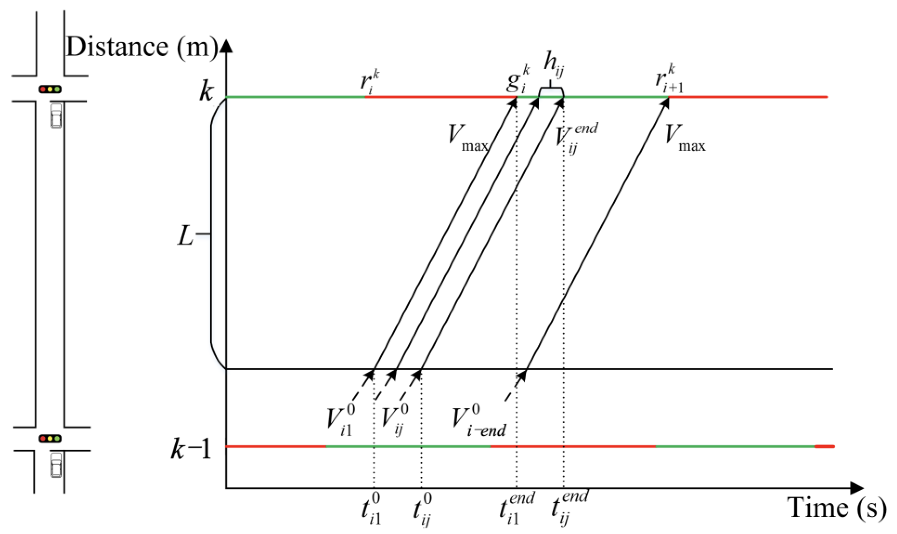
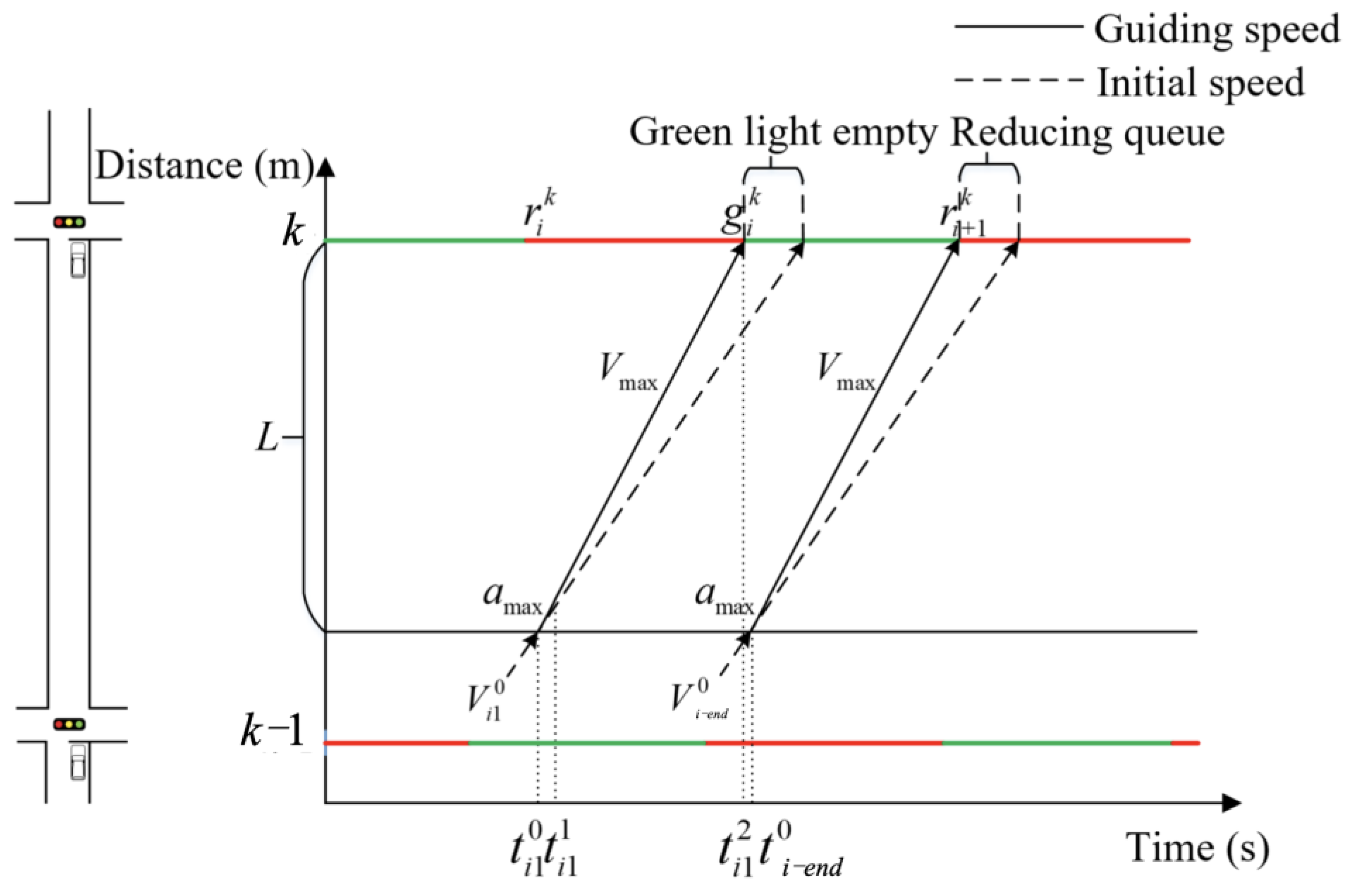
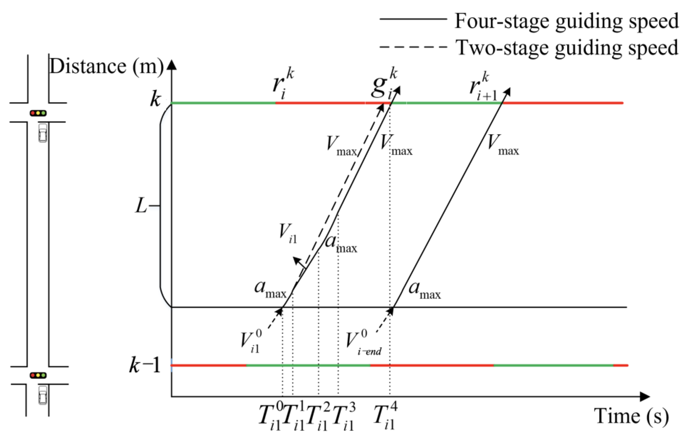
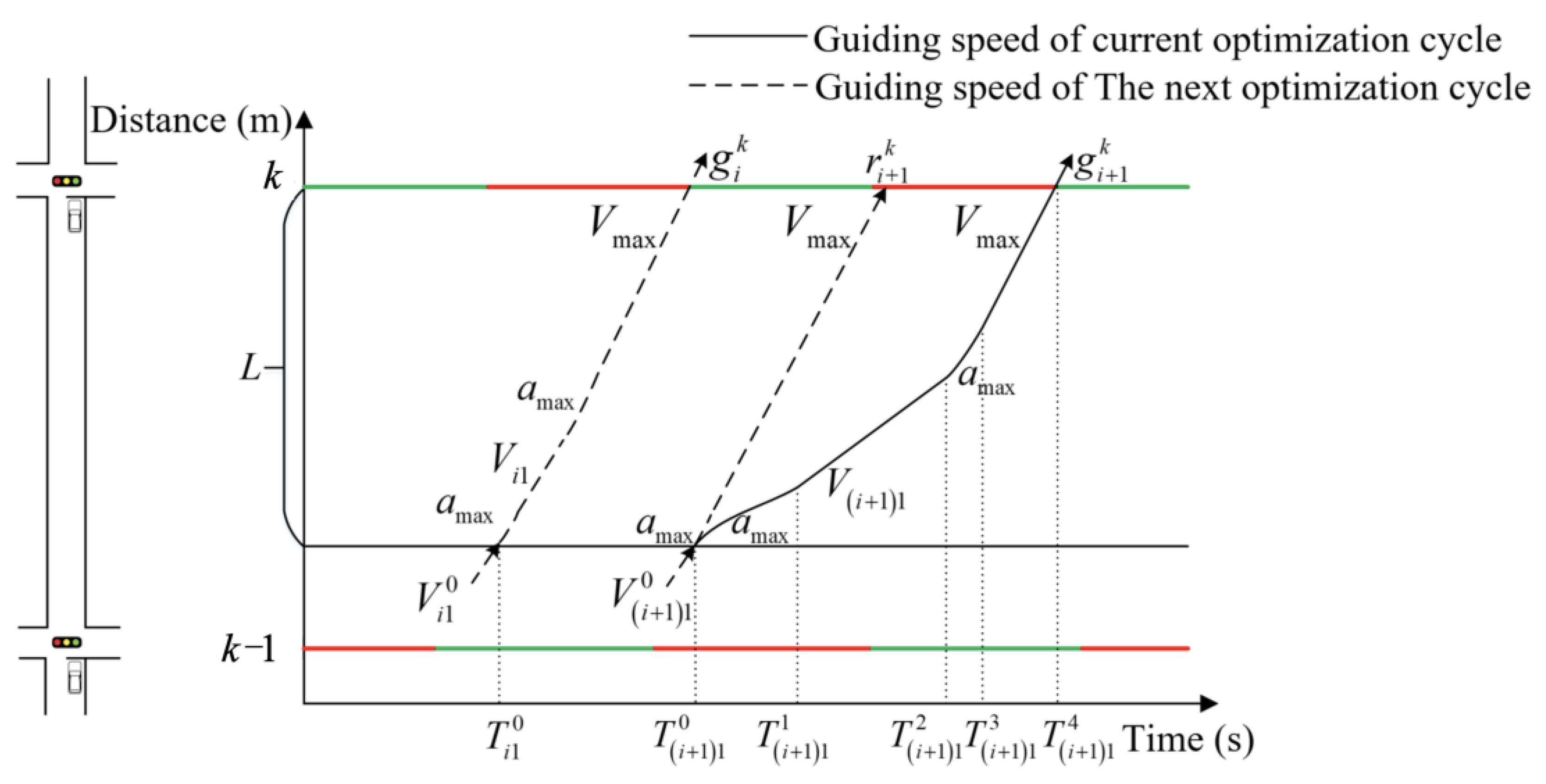
3.2.1. Vehicle Speed Guidance Strategy Under a Connected Vehicle Environment
- (a)
- Two-stage method
- (b)
- Four-stage method
- (a)
- Two-stage method
- (b)
- Four-stage method
3.2.2. Constructing the Collaborative Model Under a Connected Vehicle Environment
- (a)
- Correlation analysis of speed, signal offset and green wave bandwidth
- (b)
- Bidirectional cycle green wave bandwidth optimization
- (c)
- Model establishment
3.2.3. Calculation Method of the Collaborative Model
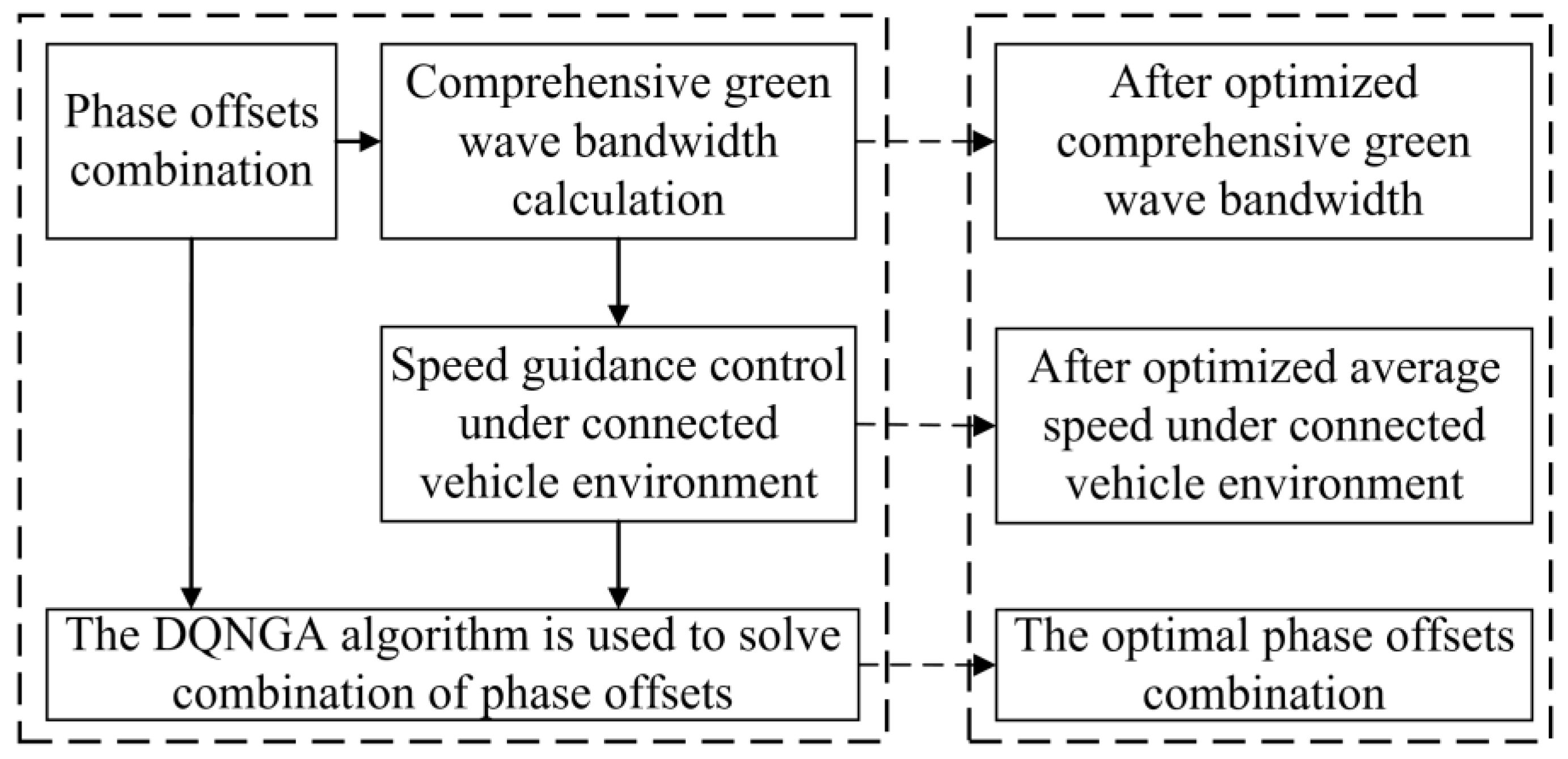
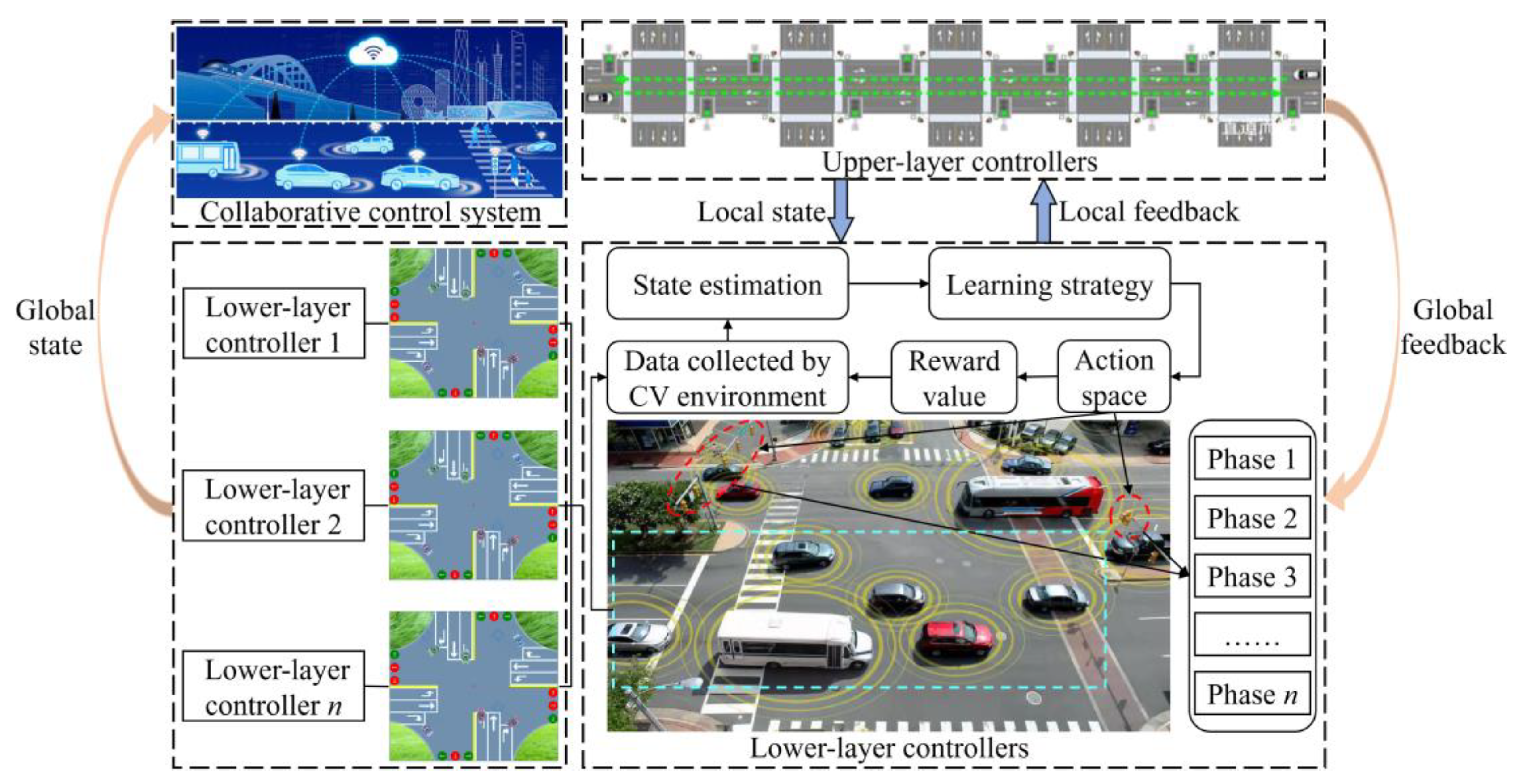
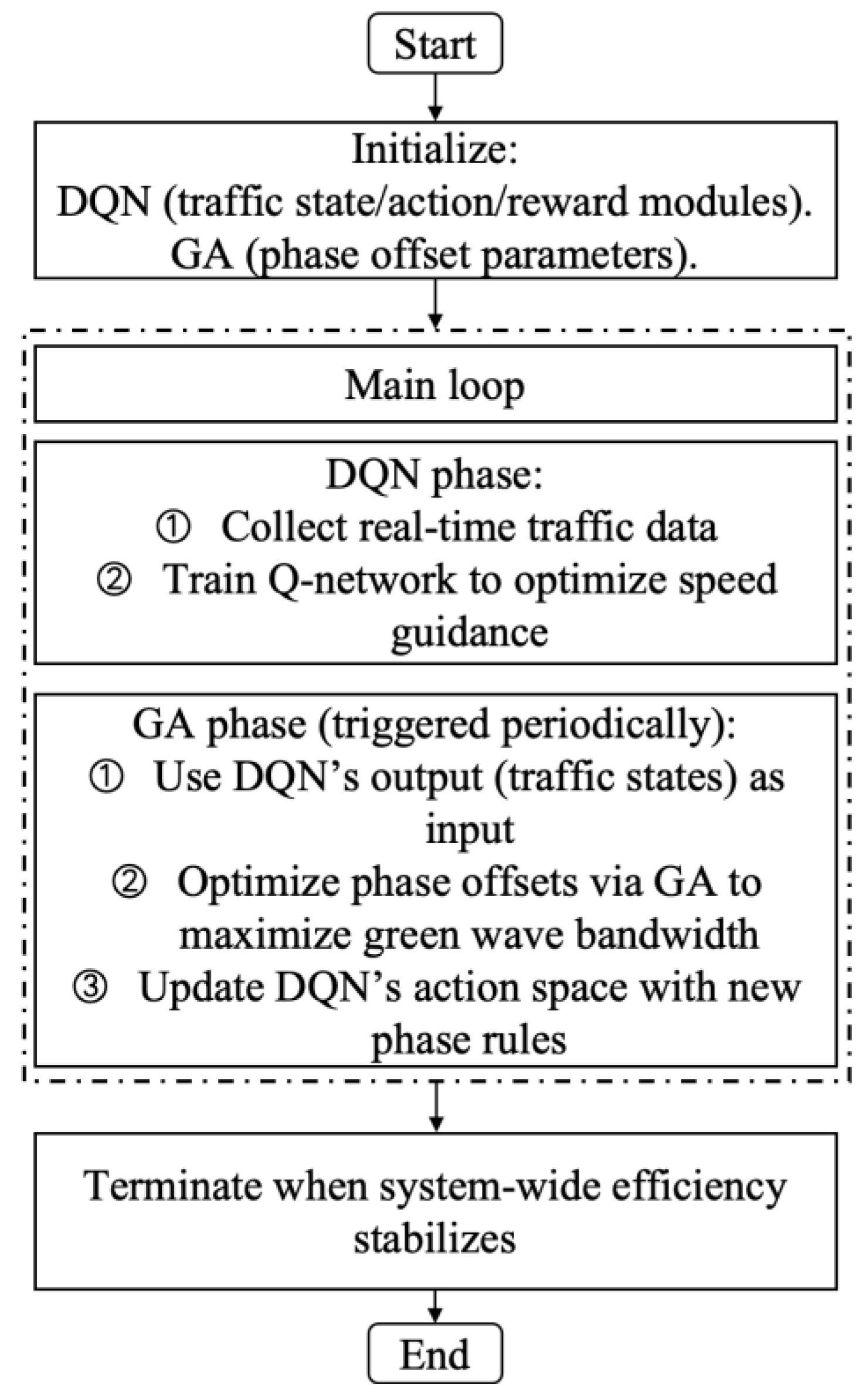
3.3. Bi-Level Combinatorial Optimization Method for Model Solving
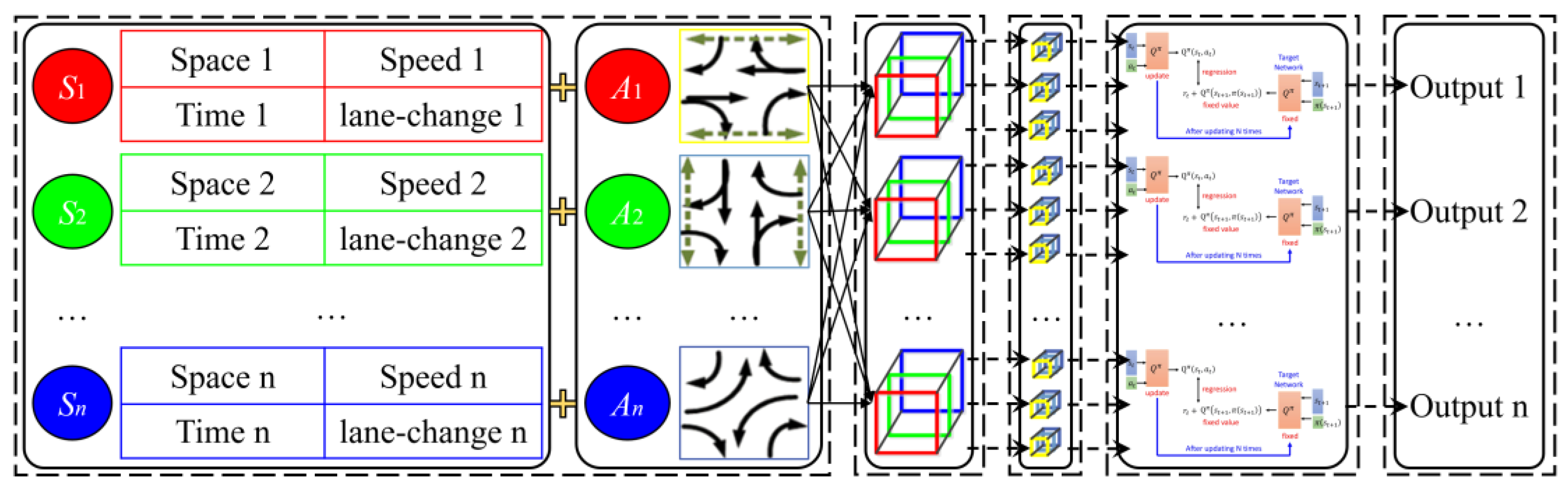
3.3.1. The Lower-Layer Control
- (a)
- State space
- (b)
- Action space
- (c)
- Reward space
| Algorithm 1 The pseudo code of DQN algorithm |
| Initialize replay memory D with capacity N |
| Initialize reward function Q with random weights θ |
| Initialize target reward function Q′ with weights θ′ |
| For episode = 1, H do |
| Initialize current state st |
| For t = 1, T do |
| With learning rate select a random action at |
| Otherwise select |
| Set next state st+1 |
| Store (st, at, , st+1) in D |
| Sample random minibatch of (st, at, , st+1) from D |
| For every (st, at, , st+1), N do Set |
| Calculate the loss function value J(θ) |
| Perform the Adaptive Moment Estimation (including (38) ~ (40)) with minimizing J(θ) to update θ |
| Every t steps, copy weights from base NN to the target NN, reset Q′ = Q |
| End For |
| End For |
| End For |
| Until training completed |
3.3.2. The Upper-Layer Control
| Algorithm 2 The procedure for GA with real number coding |
| Begin |
| Initialization: |
| { |
| Select the type of genetic operation and determine the parameters such as crossover probability and mutation probability. |
| Set evolutionary algebra counter t = 0. |
| The initial population B(0) = {O1, O2, …, ON} is generated by constructing chromosomes with phase offsets between associated intersections as genes, where N represents the population size. } |
| Measurement: select minB1 as the objective function, and then the fitness value of each individual is calculated by the initial population B(0). |
| While (the termination conditions are not satisfied) do |
| { |
| Crossover: B(t) is performed crossover operation to generate population B′(t + 1). |
| Mutation: B′(t + 1) is performed mutation operation to generate population B″(t + 1). |
| Measurement: The fitness value of each individual in population B″(t + 1) is calculated. |
| Selection: A∪B″(t + 1) is selected to generate a new population B(t + 1), where A represents a subset or empty set of B(t). |
| t = t + 1. |
| } |
| End |
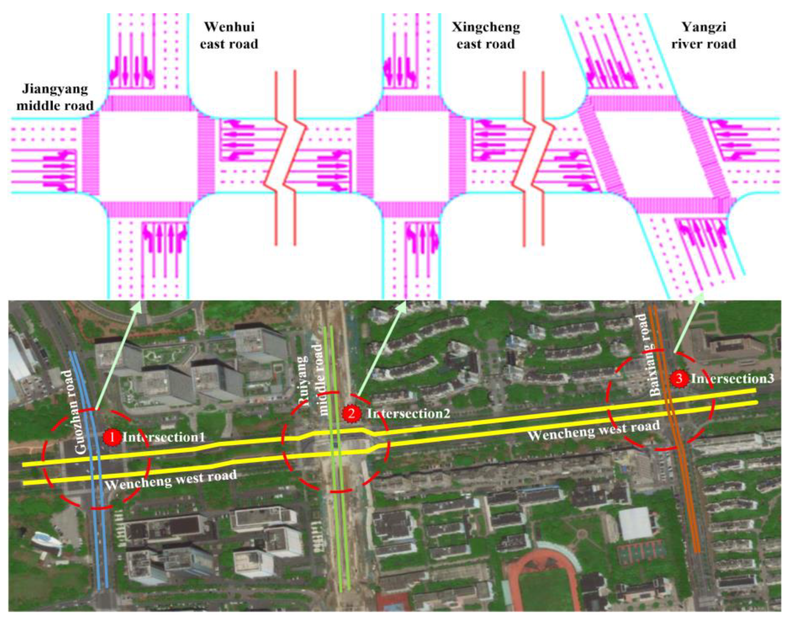
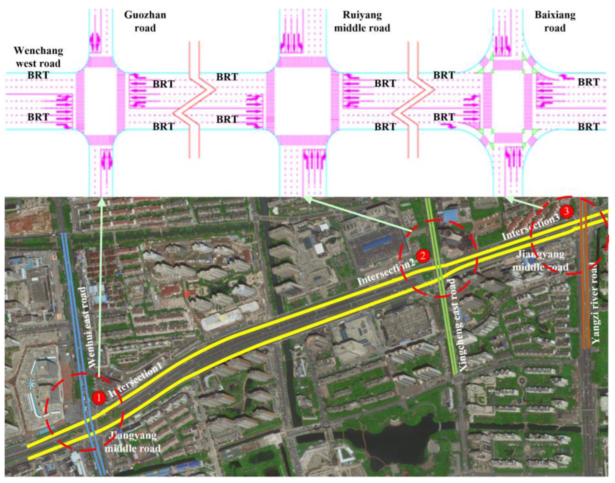
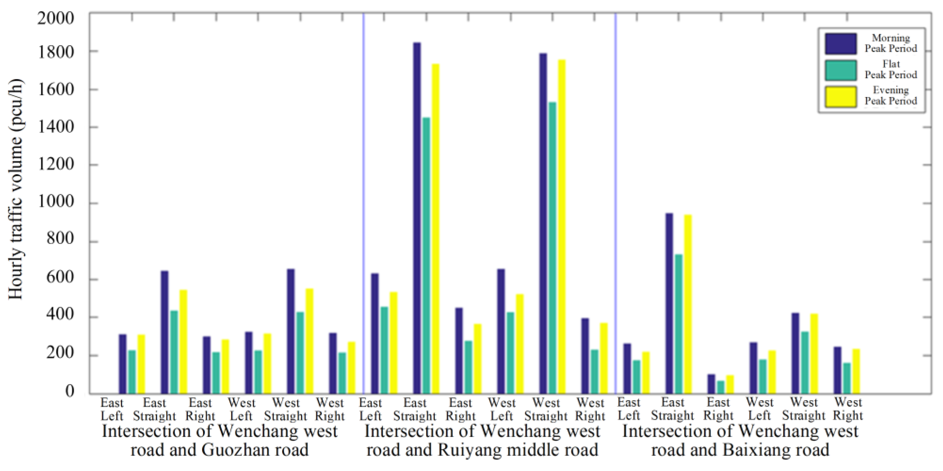
4. Case Study
4.1. Simulation Scenario
4.2. Simulation Verification
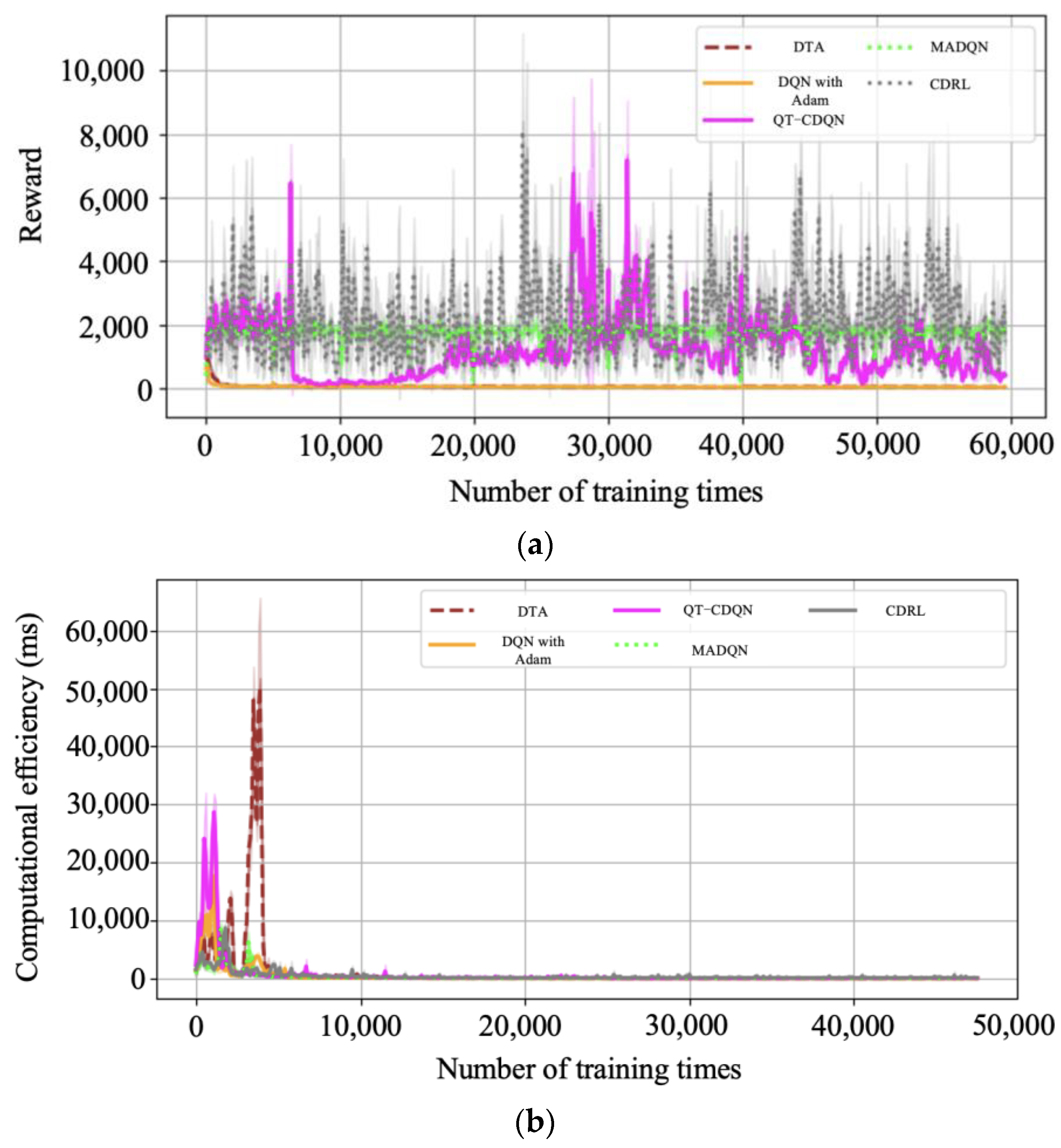
4.2.1. Results of DQN with Speed Guidance
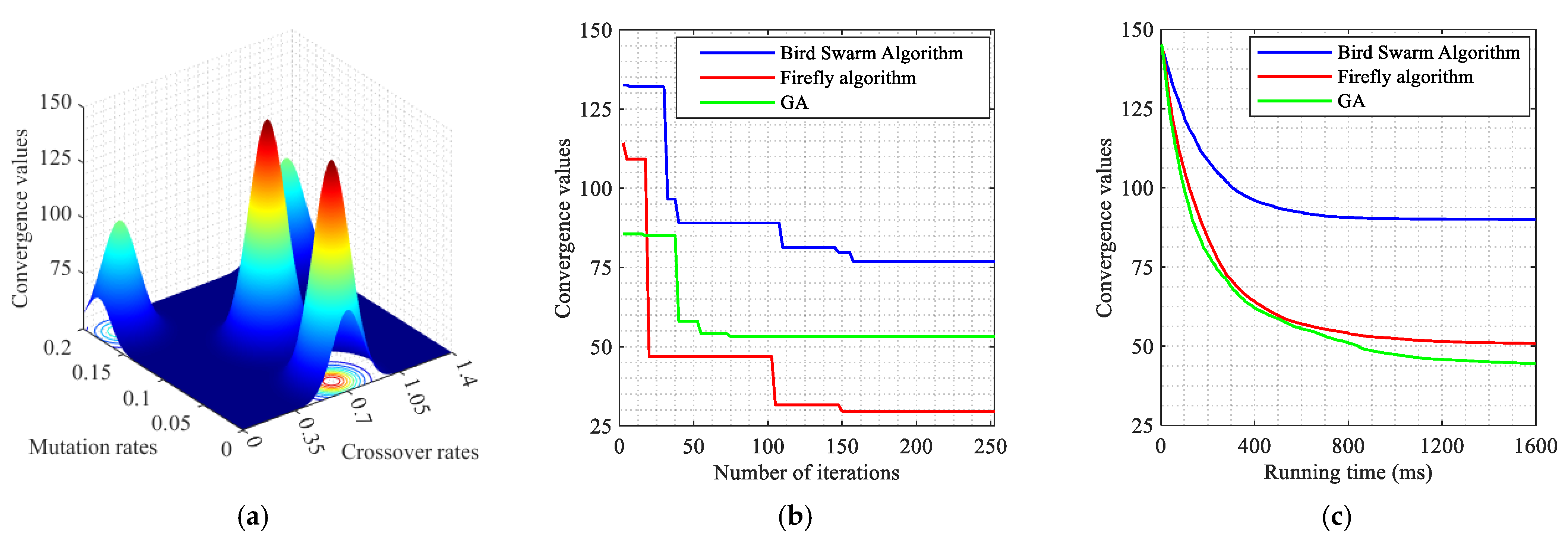
4.2.2. The Results of GA with the Bidirectional Cycle Comprehensive Green Wave Bandwidth
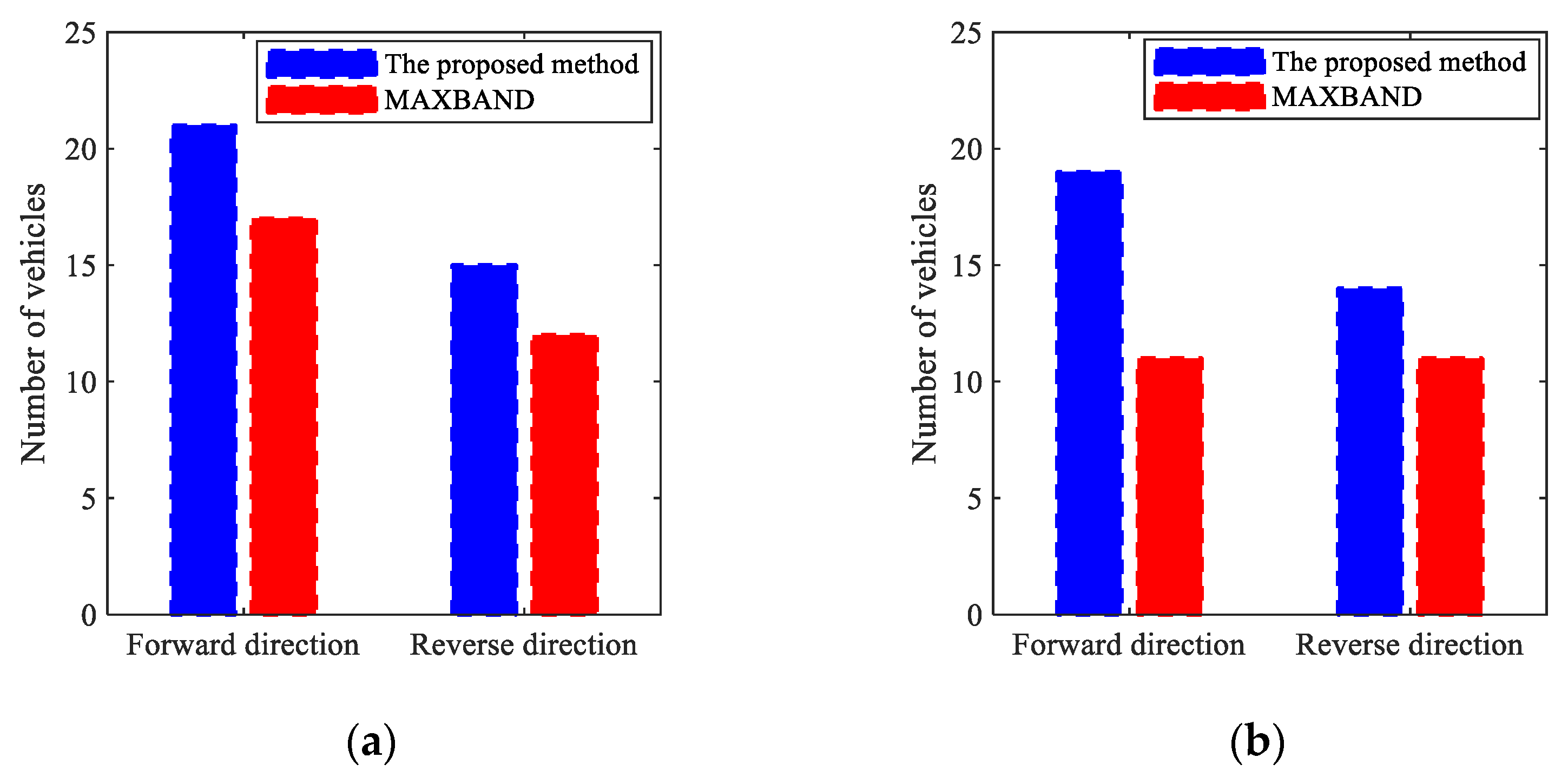
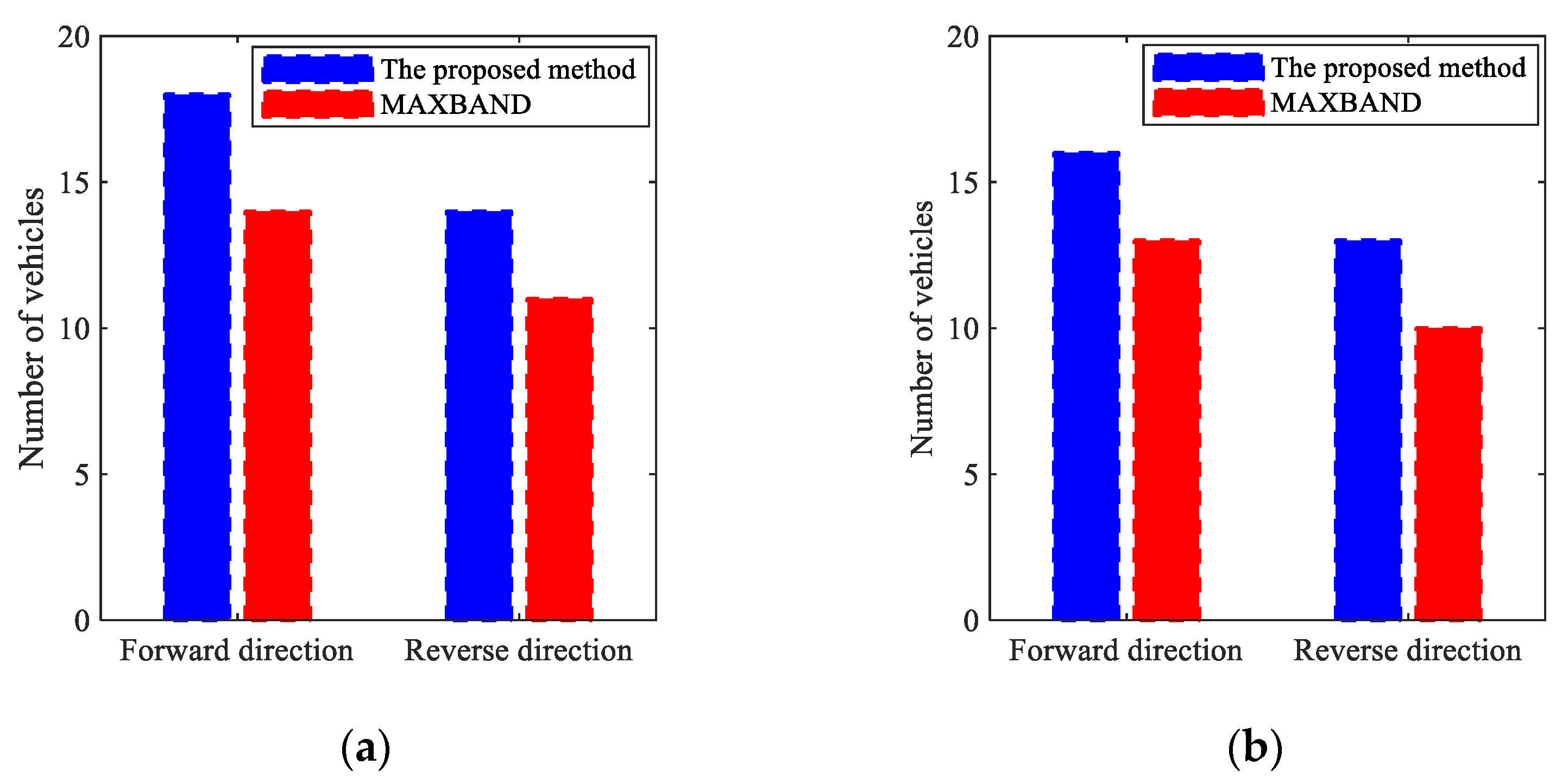
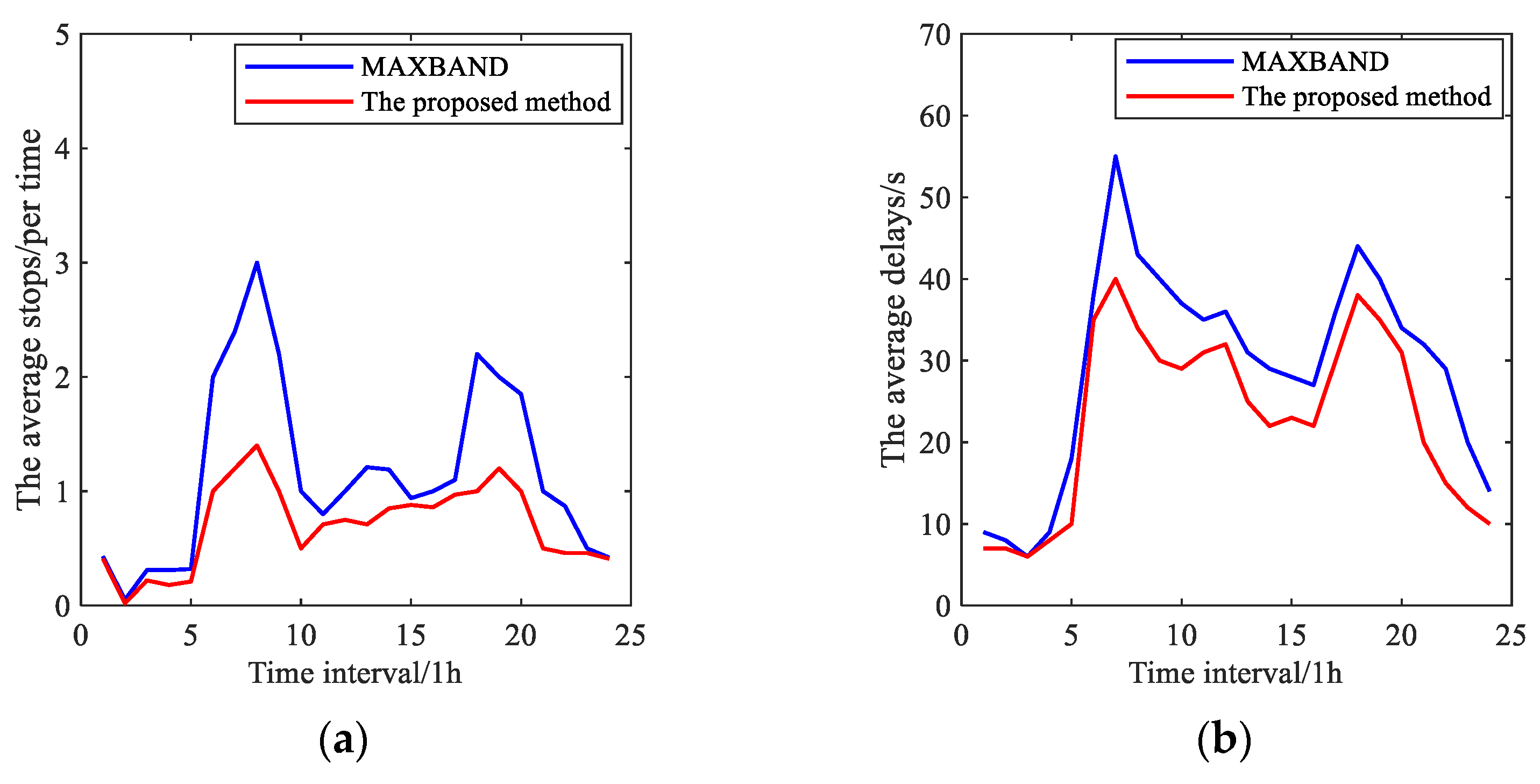
4.2.3. Simulation Results
5. Conclusions
Author Contributions
Funding
Institutional Review Board Statement
Informed Consent Statement
Data Availability Statement
Conflicts of Interest
References
- Sangkey, K.; Ali, H.; Billy, W.M.; Rouphail, N.M. Dynamic bandwidth analysis for coordinated arterial streets. J. Intell. Transp. Syst. 2016, 20, 294–310. [Google Scholar]
- Zhou, H.M.; Gene, H.H., Jr.; Zhang, Y.L. Arterial signal coordination with uneven double cycling. Transp. Res. Part A Policy Pract. 2017, 103, 409–429. [Google Scholar]
- Guler, S.I.; Menendez, M.; Meier, L. Using connected vehicle technology to improve the efficiency of intersections. Transp. Res. Part C Emerg. Technol. 2014, 46, 121–131. [Google Scholar] [CrossRef]
- Yang, K.; Menendez, M.; Guler, S.I. Implementing transit signal priority in a connected vehicle environment with and without bus stops. Transp. B Transp. Dyn. 2019, 7, 423–445. [Google Scholar]
- Xuan, Y.G.; Daganzo, C.F.; Cassidy, M.J. Increasing the capacity of signalized intersections with separate left turn phases. Transp. Res. Part B Methodol. 2011, 45, 769–781. [Google Scholar] [CrossRef]
- He, Q.; Head, K.L.; Ding, J. PAMSCOD: Platoon-based arterial multi-modal signal control with online data. Transp. Res. Part C Emerg. Technol. 2012, 20, 164–184. [Google Scholar] [CrossRef]
- Liu, Y.; Chang, G.L.; Yu, J. An Integrated Control Model for Freeway Corridor Under Nonrecurrent Congestion. IEEE Trans. Veh. Technol. 2011, 60, 1404–1418. [Google Scholar]
- Ye, L.; Wang, W.; Xing, L.; Wang, H.; Dong, C.Y. Improving traffic efficiency of highway by integration of adaptive cruise control and variable speed limit control. J. Jilin Univ. (Eng. Technol. Ed.) 2017, 47, 1420–1425. [Google Scholar]
- Zheng, J.F.; Liu, H.X. Estimating traffic volumes for signalized intersections using connected vehicle data. Transp. Res. Part C Emerg. Technol. 2017, 79, 347–362. [Google Scholar] [CrossRef]
- Sun, W.L.; Zheng, J.F.; Liu, H.X. A capacity maximization scheme for intersection management with automated vehicles. Transp. Res. Part C: Emerg. Technol. 2018, 94, 19–31. [Google Scholar] [CrossRef]
- Feng, Y.H.; Yu, C.H.; Liu, H.X. Spatiotemporal intersection control in a connected and automated vehicle environment. Transp. Res. Part C Emerg. Technol. 2018, 89, 364–383. [Google Scholar] [CrossRef]
- Yu, C.H.; Feng, Y.H.; Liu, H.X.; Ma, W.; Yang, X. Integrated optimization of traffic signals and vehicle trajectories at isolated urban intersections. Transp. Res. Part B Methodol. 2018, 112, 89–112. [Google Scholar] [CrossRef]
- Liang, X.Y.; Du, X.S.; Wang, G.L.; Han, Z. A Deep Reinforcement Learning Network for Traffic Light Cycle Control. IEEE Trans. Veh. Technol. 2019, 68, 1243–1253. [Google Scholar] [CrossRef]
- Emami, A.; Sarvi, M.; Bagloee, S.A. Network-wide traffic state estimation and rolling horizon-based signal control optimization in a connected vehicle environment. IEEE Trans. Intell. Transp. Syst. 2021, 23, 5840–5858. [Google Scholar] [CrossRef]
- Yang, K.D.; Menendez, M.; Zheng, N. Heterogeneity aware urban traffic control in a connected vehicle environment: A joint framework for congestion pricing and perimeter control. Transp. Res. Part C Emerg. Technol. 2019, 105, 439–455. [Google Scholar] [CrossRef]
- Rafter, C.B.; Anvari, B.; Box, S.; Cherrett, T. Augmenting Traffic Signal Control Systems for Urban Road Networks with Connected Vehicles. IEEE Trans. Intell. Transp. Syst. 2020, 21, 1728–1740. [Google Scholar] [CrossRef]
- Mohebifard, R.; Hajbabaie, A. Optimal network-level traffic signal control: A benders decomposition-based solution algorithm. Transp. Res. Part B Methodol. 2019, 121, 252–274. [Google Scholar] [CrossRef]
- Kamal, M.A.S.; Mukai, M.; Murata, J.; Kawabe, T. Model Predictive Control of Vehicles on Urban Roads for Improved Fuel Economy. IEEE Trans. Control Syst. Technol. 2013, 21, 831–841. [Google Scholar] [CrossRef]
- Wu, W.; Li, P.K.; Zhang, Y. Modelling and Simulation of Vehicle Speed Guidance in Connected Vehicle Environment. Int. J. Simul. Model. 2015, 14, 145–157. [Google Scholar] [CrossRef]
- Lin, P.Q.; Zhuo, Q.F.; Yao, K.B.; Ran, B.; Xu, J. Solving and Simulation of Microcosmic Control Model of Intersection Traffic Flow in Connected-vehicle Network Environment. China J. Highw. Transp. 2015, 28, 82–90. [Google Scholar]
- Ma, W.; Zou, L.; An, K.; Gartner, N.H.; Wang, M. A partition-enabled multi-mode band approach to arterial traffic signal optimization. IEEE Trans. Intell. Transp. Syst. 2019, 20, 313–322. [Google Scholar]
- Xu, B.; Ban, X.J.; Bian, Y.; Li, W.; Wang, J.; Li, S.E.; Li, K. Cooperative method of traffic signal optimization and speed control of connected vehicles at isolated intersections. IEEE Trans. Intell. Transp. Syst. 2019, 20, 1390–1403. [Google Scholar]
- Wu, L.N.; Ci, Y.S.; Sun, Y.C.; Qi, W. Research on Joint Control of On-Ramp Metering and Mainline Speed Guidance in the Urban Expressway Based on MPC and Connected Vehicles. J. Adv. Transp. 2020, 2020, 7518087. [Google Scholar]
- Zhou, A.; Peeta, S.; Yang, M.; Wang, J. Cooperative signal-free intersection control using virtual platooning and traffic flow regulation. Transp. Res. Part C Emerg. Technol. 2022, 138, 103610. [Google Scholar]
- Chen, X.; Hu, M.; Xu, B.; Bian, Y.; Qin, H. Improved reservation-based method with controllable gap strategy for vehicle coordination at non-signalized intersections. Phys. A Stat. Mech. its Appl. 2022, 604, 127953. [Google Scholar]
- Liang, X.; Guler, S.I.; Gayah, V.V. Decentralized arterial traffic signal optimization with connected vehicle information. J. Intell. Transp. Syst. 2021, 27, 145–160. [Google Scholar]
- Chen, H.; Qiu, T.Z. Distributed Dynamic Route Guidance and Signal Control for Mobile Edge Computing-Enhanced Connected Vehicle Environment. IEEE Trans. Intell. Transp. Syst. 2022, 23, 12251–12262. [Google Scholar]
- Yang, K.D.; Zheng, N.; Menendez, M. Multi-scale Perimeter Control Approach in a Connected-Vehicle Environment. Transp. Res. Procedia 2017, 23, 101–120. [Google Scholar]
- Wang, M.; Daamen, W.; Hoogendoorn, S.P.; van Arem, B. Rolling horizon control framework for driver assistance systems. Part I: Mathematical formulation and non-cooperative systems. Transp. Res. Part C Emerg. Technol. 2014, 40, 271–289. [Google Scholar]
- Ubiergo, G.A.; Jin, W.L. Mobility and environment improvement of signalized networks through Vehicle-to-Infrastructure (V2I) communications. Transp. Res. Part C Emerg. Technol. 2016, 68, 70–82. [Google Scholar]
- Wan, N.; Vahidi, A.; Luckow, A. Optimal speed advisory for connected vehicles in arterial roads and the impact on mixed traffic. Transp. Res. Part C Emerg. Technol. 2016, 69, 548–563. [Google Scholar] [CrossRef]
- Liu, X.; Xu, J.; Zheng, K.; Zhang, G.; Liu, J.; Shiratori, N. Throughput Maximization with an AoI Constraint in Energy Harvesting D2D-Enabled Cellular Networks: An MSRA-TD3 Approach. IEEE Trans. Wirel. Commun. 2025, 24, 1448–1466. [Google Scholar]
- He, X.; Liu, H.X.; Liu, X. Optimal vehicle speed trajectory on a signalized arterial with consideration of queue. Transp. Res. Part C Emerg. Technol. 2015, 61, 106–120. [Google Scholar]
- Tang, T.Q.; Yi, Z.Y.; Zhang, J.; Wang, T.; Leng, J.Q. A speed guidance strategy for multiple signalized intersections based on car-following model. Phys. A Stat. Mech. its Appl. 2018, 496, 399–409. [Google Scholar]
- Zhao, S.; Zhang, K. Online predictive connected and automated eco-driving on signalized arterials considering traffic control devices and road geometry constraints under uncertain traffic conditions. Transp. Res. Part B Methodol. 2021, 145, 80–117. [Google Scholar]
- He, Z.C.; Kang, H.; Li, E.; Zhou, E.L.; Cheng, H.T.; Huang, Y.Y. Coordinated control of heterogeneous vehicle platoon stability and energy-saving control strategies. Phys. A Stat. Mech. its Appl. 2022, 606, 128155. [Google Scholar]
- Wu, W.; Ma, W.J.; Yang, X.G. Dynamic speed-based signal offset optimization model within vehicle infrastructure integration environment. Control Theory Appl. 2014, 31, 519–524. [Google Scholar]
- Tajalli, M.; Hajbabaie, A. Distributed optimization and coordination algorithms for dynamic speed optimization of connected and autonomous vehicles in urban street networks. Transp. Res. Part C Emerg. Technol. 2018, 95, 497–515. [Google Scholar]
- Wang, P.W.; Jiang, Y.L.; Lin, X.; Zhao, Y.; Li, Y. A joint control model for connected vehicle platoon and arterial signal coordination. J. Intell. Transp. Syst. 2020, 24, 81–92. [Google Scholar]
- Bie, Y.M.; Xiong, X.Y.; Yan, Y.D.; Qu, X. Dynamic headway control for high-frequency bus line based on speed guidance and intersection signal adjustment. Comput.-Aided Civ. Infrastruct. Eng. 2020, 35, 4–25. [Google Scholar]
- Liu, J.H.; Lin, P.Q.; Ran, B. A Reservation-Based Coordinated Transit Signal Priority Method for Bus Rapid Transit System with Connected Vehicle Technologies. IEEE Intell. Transp. Syst. Mag. 2020, 13, 17–30. [Google Scholar]
- Lu, K.; Tian, X.; Jiang, S.Y.; Xu, J.M.; Wang, Y.H. Optimization model for regional green wave coordinated control based on ring-and-barrier structure. J. Intell. Transp. Syst. 2020, 26, 68–80. [Google Scholar]
- Lu, K.; Tian, X.; Jiang, S.; Lin, Y.; Zhang, W. Optimization Model of Regional Green Wave Coordination Control for the Coordinated Path Set. IEEE Trans. Intell. Transp. Syst. 2023, 24, 7000–7011. [Google Scholar]
- Milanes, V.; Shladover, S.E. Modeling cooperative and autonomous adaptive cruise control dynamic responses using experimental data. Transp. Res. Part C Emerg. Technol. 2014, 48, 285–300. [Google Scholar]
- Al-Jhayyish, A.M.H.; Schmidt, K.W. Feedforward Strategies for Cooperative Adaptive Cruise Control in Heterogeneous Vehicle Strings. IEEE Trans. Intell. Transp. Syst. 2018, 19, 113–122. [Google Scholar]
- Rajamani, R. Vehicle Dynamics and Control; Springer: Berlin/Heidelberg, Germany, 2011. [Google Scholar]
- Ploeg, J.; Scheepers, B.T.M.; van Nunen, E.; van de Wouw, N.; Nijmeijer, H. Design and experimental evaluation of cooperative adaptive cruise control. In Proceedings of the 14th International IEEE Conference on Intelligent Transportation Systems (ITSC), Washington, DC, USA, 5–7 October 2011; pp. 260–265. [Google Scholar]
- Segata, M.; Bloessl, B.; Joerer, S.; Sommer, C.; Dressler, F. Towards inter-vehicle communication strategies for platooning support. In Proceedings of the 7th International Workshop on Communication Technologies for Vehicles (Nets4Cars-Fall), St. Petersburg, Russia, 6–8 October 2014; pp. 1–6. [Google Scholar]
- Ma, D.F.; Chen, X.; Wu, X.D.; Jin, S. Mixed-coordinated Decision-making Method for Arterial Signals Based on Reinforcement Learning. J. Transp. Syst. Eng. Inf. Technol. 2022, 22, 145–153. [Google Scholar]
- Liu, X.M.; Tang, S.H. Green Wave Coordinated Control Method Based on Continuously Passing Vehicles. J. Transp. Syst. Eng. Inf. Technol. 2012, 12, 34–40. [Google Scholar]
- Kingma, D.P.; Ba, J. Adam: A method for stochastic optimization. arXiv 2014, arXiv:1412.6980. [Google Scholar]
- Van der Pol, E.; Oliehoek, F.A. Coordinated Deep Reinforcement Learners for Traffic Light Control. In Proceedings of the Learning, Inference and Control of Multi-Agent Systems (at NIPS 2016), Barcelona, Spain, 5–10 December 2016; Volume 8, pp. 21–38. [Google Scholar]
- Gao, J.; Shen, Y.; Liu, J.; Ito, M.; Shiratori, N. Adaptive traffic signal control: Deep reinforcement learning algorithm with experience replay and target network. arXiv 2017, arXiv:1705.02755. [Google Scholar]
- Ge, H.; Song, Y.; Wu, C.; Ren, J.; Tan, G. Cooperative deep Q-learning with Q-value transfer for multi-intersection signal control. IEEE Access 2019, 7, 40797–40809. [Google Scholar]
- Kodama, N.; Harada, T.; Miyazaki, K. Traffic Signal Control System Using Deep Reinforcement Learning with Emphasis on Reinforcing Successful Experiences. IEEE Access 2022, 10, 128943–128950. [Google Scholar]
- Meng, X.B.; Gao, X.Z.; Lu, L.; Liu, Y.; Zhang, H. A new bio-inspired optimisation algorithm: Bird Swarm Algorithm. J. Exp. Theor. Artif. Intell. 2016, 28, 673–687. [Google Scholar]
- Wu, J.; Wang, Y.G.; Burrage, K.; Tian, Y.C.; Lawson, B.; Ding, Z. An improved firefly algorithm for global continuous optimization problems. Expert Syst. Appl. 2020, 149, 113340. [Google Scholar]


| Symbol | Quantity |
|---|---|
| i | The ith optimization cycle |
| j | The jth vehicle |
| The target speed of the vehicle within the control range, m/s | |
| Maximum permissible vehicle speed, m/s | |
| The target time of vehicle arrival at downstream intersection, s | |
| The time headway between the current vehicle and the preceding vehicle, s | |
| The target displacement of the vehicle within the control range, m | |
| The time safe headway, s | |
| The safe parking distance, m | |
| The front vehicle’s length of the current vehicle, m | |
| The initial speed of the vehicle entering the control range, m/s | |
| The initial speed of the last vehicle entering the control range in the optimization cycle, m/s | |
| The initial time of vehicle entering the control range, s | |
| The time when the vehicle reaches the downstream intersection, s | |
| The time when the vehicle is at the end of the first uniform speed change stage, s | |
| The time when the vehicle ends its first uniform motion at the guiding speed, s | |
| The time when the vehicle is at the end of the second uniform speed change stage, s | |
| The total displacement of the vehicle within the control range, m | |
| The displacement of vehicle during the first uniform speed change stage, m | |
| The displacement of the vehicle in the stage of uniform motion at Vmax, m | |
| The displacement of the vehicle during the first uniform motion stage at the guiding speed, m | |
| The displacement of the vehicle during the second uniform speed change stage, m | |
| The guiding speed of the vehicle entering the control range, m/s | |
| The time distance function between the current vehicle and the front vehicle | |
| The time distance function of the front vehicle | |
| The time distance function of the current vehicle | |
| The safe space headway, m | |
| The initial time when the last vehicle enters the control range in the optimization cycle, s | |
| P | The control objective expression of forward green wave bandwidth. |
| H | The control objective expression of reverse green wave bandwidth. |
| Variable | Definition |
|---|---|
| tc | The time when the cth gather–disperse wave intersects with the c − 1th gather–disperse wave at the downstream intersection |
| v1 | The average speed corresponding to traffic flow qg2 |
| v2 | The average speed corresponding to traffic flow qr1 |
| v3 | The average speed corresponding to traffic flow qr2 |
| v4 | The average speed corresponding to traffic flow qg1 |
| W1~W5 | The gather–disperse wave speed |
| qg1 | The saturation flow of queuing vehicles in coordinated phase when they release |
| qg2 | The average flow of vehicles flowing out after the queue of vehicles has dissipated late in the green light of coordinated phase |
| qr1 | The average flow of queuing vehicles driving out of the intersection in the pre-reddish phase of the coordinated phase interface with the non-coordinated phase |
| qr2 | The average vehicle outflow after the coordinated phase red time late articulated uncoordinated phase queue has dissipated |
| tg1 | The time for the vehicle queue to dissipate during the green time of coordinated phase |
| tr1 | The time for completion of uncoordinated phase queue dissipation for coordinated phase articulation |
| C′ | Public cycle of upstream and downstream intersections |
| Tg | The upstream intersections with the green time of the coordinated phases |
| Tr | The upstream intersections with the red time of the coordinated phases |
| Tgb | Time difference between the beginning of the green wave at the upstream intersection and the beginning of the green time at the coordinated phase in the same cycle |
| Tge | The time difference between the end of the green wave at the upstream intersection and the start of the green light at the coordinated phase in the same cycle |
| Vehicle_ID | Global_Time | Local_X | Local_Y | Global_X | Global_Y | v | Lane_ID | Following | Space_Headway | Time_Headway |
|---|---|---|---|---|---|---|---|---|---|---|
| 515 | 1,118,848,075,000 | 30.034 | 188.062 | 6,451,203.729 | 1,873,252.549 | 13 | 3 | 523 | 119.1 | 5.11 |
| 2224 | 1,113,437,421,700 | 41.429 | 472.901 | 6,042,814.264 | 2,133,542.012 | 14 | 4 | 2211 | 53.34 | 2.01 |
| 1033 | 1,118,848,324,700 | 6.202 | 1701.14 | 6,452,347.673 | 1,872,258.452 | 13 | 1 | 1040 | 38.81 | 0.92 |
| 744 | 1,118,848,181,200 | 28.878 | 490.086 | 6,451,422.353 | 1,873,041.018 | 15 | 3 | 752 | 37.8 | 1.54 |
| … | … | … | … | … | … | … | … | … | … | … |
| Model Parameters | Value |
|---|---|
| Replay memory D | 40,000 |
| The number of training times | 80,000 |
| Batch size | 64 |
| Learning rate | 0.0001 |
| Discount rate | [0.01, 0.99] |
| ReLU activation function | 0.001 |
| /s | 3 |
| Road Section | Intersection | Signal Offset of MAXBAND | Signal Offset of the Proposed Model | Forward and Reverse Comprehensive Green Wave Bandwidth of MAXBAND | Forward and Reverse Comprehensive Green Wave Bandwidth of the Proposed Model |
|---|---|---|---|---|---|
| Jiangyang Middle Road Section | Intersection of Jiangyang Middle Road and Huidong Road | 0 | 15 | (30, 27) | (34, 30) |
| Intersection of Jiangyang Middle Road and Xingcheng East Road | 126 | 112 | |||
| Intersection of Jiangyang Middle Road and Yangzi River Road | 77 | 85 | |||
| Wenchang West Road Section | Intersection of Wenchang West Road and Guozhan Road | 72 | 77 | (21, 18) | (23, 21) |
| Intersection of Wenchang West Road and Ruiyang Middle Road | 0 | 11 | |||
| Intersection of Wenchang West Road and Baixiang Road | 45 | 38 |
| Road Section | Intersection | Signal Offset of MAXBAND | Signal Offset of the Proposed Model | Forward and Reverse Comprehensive Green Wave Bandwidth of MAXBAND | Forward and Reverse Comprehensive Green Wave Bandwidth of the Proposed Model |
|---|---|---|---|---|---|
| Jiangyang Middle Road Section | Intersection of Jiangyang Middle Road and Huidong Road | 0 | 113 | (35, 33) | (38, 35) |
| Intersection of Jiangyang Middle Road and Xingcheng East Road | 63 | 78 | |||
| Intersection of Jiangyang Middle Road and Yangzi River Road | 117 | 101 | |||
| Wenchang West Road Section | Intersection of Wenchang West Road and Guozhan Road | 36 | 28 | (26, 24) | (28, 27) |
| Intersection of Wenchang West Road and Ruiyang Middle Road | 0 | 119 | |||
| Intersection of Wenchang West Road and Baixiang Road | 45 | 52 |
| Road Section | Intersection | Signal Offset of MAXBAND | Signal Offset of the Proposed Model | Forward and Reverse Comprehensive Green Wave Bandwidth of MAXBAND | Forward and Reverse Comprehensive Green Wave Bandwidth of the Proposed Model |
|---|---|---|---|---|---|
| Jiangyang Middle Road Section | Intersection of Jiangyang Middle Road and Huidong Road | 0 | 17 | (29, 26) | (32, 29) |
| Intersection of Jiangyang Middle Road and Xingcheng East Road | 126 | 118 | |||
| Intersection of Jiangyang Middle Road and Yangzi River Road | 77 | 91 | |||
| Wenchang West Road Section | Intersection of Wenchang West Road and Guozhan Road | 72 | 82 | (23, 20) | (26, 24) |
| Intersection of Wenchang West Road and Ruiyang Middle Road | 0 | 11 | |||
| Intersection of Wenchang West Road and Baixiang Road | 45 | 35 |
| Road Section | Average Stops | Average Delay | ||||
|---|---|---|---|---|---|---|
| MAXBAND | The Proposed Model | Improvement Effect | MAXBAND | The Proposed Model | Improvement Effect | |
| Morning Peak Period | 2.75 | 1.277 | 53.56% | 53 | 43 | 18.87% |
| Flat Peak Period | 1.121 | 0.693 | 38.18% | 37 | 28 | 24.32% |
| Evening Peak Period | 2.295 | 1.224 | 46.67% | 47 | 37 | 21.28% |
| Road Section | Average Stops | Average Delay | ||||
|---|---|---|---|---|---|---|
| MAXBAND | The Proposed Model | Improvement Effect | MAXBAND | The Proposed Model | Improvement Effect | |
| Morning Peak Period | 3.9 | 1.95 | 50.00% | 57 | 42 | 28.85% |
| Flat Peak Period | 1.913 | 1.212 | 36.64% | 36 | 30 | 16.67% |
| Evening Peak Period | 3.25 | 1.888 | 41.91% | 48 | 41 | 14.58% |
| Road Section | Metric | MAXBAND | MULTIBAND | PPO | Proposed DQNGA |
|---|---|---|---|---|---|
| Jiangyang Middle | Average. Delay (s) | 53 | 48 | 45 | 37 |
| Wenchang West | Average. Stops | 3.9 | 3.2 | 2.8 | 1.95 |
Disclaimer/Publisher’s Note: The statements, opinions and data contained in all publications are solely those of the individual author(s) and contributor(s) and not of MDPI and/or the editor(s). MDPI and/or the editor(s) disclaim responsibility for any injury to people or property resulting from any ideas, methods, instructions or products referred to in the content. |
© 2025 by the authors. Licensee MDPI, Basel, Switzerland. This article is an open access article distributed under the terms and conditions of the Creative Commons Attribution (CC BY) license (https://creativecommons.org/licenses/by/4.0/).
Share and Cite
Dong, L.; Xie, X.; Zhang, L.; Li, S.; Yang, Z. A Multi-Level Speed Guidance Cooperative Approach Based on Bidirectional Periodic Green Wave Coordination Under Intelligent and Connected Environment. Sensors 2025, 25, 2114. https://doi.org/10.3390/s25072114
Dong L, Xie X, Zhang L, Li S, Yang Z. A Multi-Level Speed Guidance Cooperative Approach Based on Bidirectional Periodic Green Wave Coordination Under Intelligent and Connected Environment. Sensors. 2025; 25(7):2114. https://doi.org/10.3390/s25072114
Chicago/Turabian StyleDong, Luxi, Xiaolan Xie, Lieping Zhang, Shuiwang Li, and Zhiqian Yang. 2025. "A Multi-Level Speed Guidance Cooperative Approach Based on Bidirectional Periodic Green Wave Coordination Under Intelligent and Connected Environment" Sensors 25, no. 7: 2114. https://doi.org/10.3390/s25072114
APA StyleDong, L., Xie, X., Zhang, L., Li, S., & Yang, Z. (2025). A Multi-Level Speed Guidance Cooperative Approach Based on Bidirectional Periodic Green Wave Coordination Under Intelligent and Connected Environment. Sensors, 25(7), 2114. https://doi.org/10.3390/s25072114